Sharif University of Technology
Scientia IranicaTransactions A: Civil Engineering www.scientiairanica.com
Study of rotational kinematic hardening model: A
general plasticity formula and model implement
K.M. Wei
a;b;and Sh. Zhu
a;ba. Institute of Hydraulic Structures, Hohai University, Xikang Road 1, Nanjing 210098, PR China.
b. State Key Laboratory of Hydrology, Water Resources and Hydraulic Engineering, Hohai University, Nanjing 210098, PR China. Received 17 July 2012; accepted 28 January 2013
KEYWORDS Elastoplasticity; Rotational kinematic hardening model; Stress reversal; General plasticity formula;
Logical procedures.
Abstract.Theories of the rotational kinematic hardening model are introduced in detail. This model is used to predict soil behaviors under large stress reversals by incorporating the rotation and intersection of isotropic hardening yield surfaces in principal stress space. During the monotonic loading, the model behaves the same as isotropic hardening model, but once stress reversals occurs, new kinematic yield surfaces will generate, then these yield surfaces evolve (e.g. rotate, shrink, expand, vanish etc.) obeying the rotational kinematic hardening rule in the process of loading. A general plasticity formula of rotated yield surface or plastic potential surface in the principal stress space is given in this research, which is the basis of the rotational kinematic hardening model. It is also a very integral part to design logical procedures to determine the load mode of soil element during surfaces' evolution. New logical procedures developed by this paper have been successfully used within the framework of Lade-Kim model; test results and model predictions showed a good consistency in stress reversal triaxial tests, using loose Santa Monica beach sand. Source codes of logical procedures to implement the rotational kinematic hardening model within the framework of Lade-Kim model are provided at the end of this paper to give readers a further understanding.
c
2013 Sharif University of Technology. All rights reserved.
1. Introduction
A reasonable prediction of soil deformation under various types of loading is of increasing importance for practical problems in engineering. Many models were developed in the past years under the conventional theory of plasticity (e.g. [1-5]). These models could give satisfying description of soil behaviors under monotonic loading, however, they are incapable of predicting large stress reversal and cyclic loading, which attracts great attention in earthquake engineering and oshore structure [6,7]. With the rapid development of design requirements, structures that suer from large stress
*. Corresponding author.
E-mail address: [email protected] (K.M. Wei)
reversal or cyclic loading should be analyzed using new theories.
Conventional plasticity theory assumed that the domain enclosed by the yield surface is totally elastic, thus only elastic deformation could occur within the yield surface during stress reversals. Plastic deforma-tion would not be generated during the unloading and loading process until the stress penetrates the current yield surface. However, many test results indicated that large stress reversals in particle materials [8,9] or metals [10] all results in plastic deformation (e.g. in the process of unloading and reloading, a stress-strain curve with a closed hysteresis loop will form). Currently, it is a tendency to extend plasticity theory to reect this part of plastic deformation within the yield surface.
Dafalias and Popov [11-13] rst introduced the two surfaces model for complex loading of metals, and Dafalias [14,15] generalized it to the framework of \bounding surface model" for any materials. In the meantime, Hashiguchi et al. [16-25] proposed the concept of \subloading". Both the \subloading" model and \bounding surface" model are two surface models with the outer yield surface called \normal yield sur-face" or \bounding sursur-face", the inner surface called \subloading surface" or \loading surface". The dier-ences of these two models are that dierent methods are used to get plastic modulus of the current stress point. In the bounding surface model, plastic deforms at any interior points of the bounding surface, where plastic modulus is obtained by interpolation from the \image point", according to the geometric distance in the stress space, proper \mapping rule"(e.g. radical mapping rule) should be predened to map the current stress point to the \image point" on the bounding surface, while in the \subloading surface" model, the plastic modulus of the current stress point is obtained using the consistency condition of the \subloading surface". In recent years, \bounding surface" or \subloading surface" concept was used to improve the existing models by many scholars. Andrianopoulos et al. [26] incorporated the critical state soil mechanics with the bounding surface model to simulate earthquake soil liquefaction. Suebsuk et al. [27] improved Structured Cam Clay (SCC) model with concept of bounding surface for overconsolidated structured clays. Nakai and Hinokio [28] expanded the tij-clay model with
the concept of subloading surface concept to reect the density or conning pressure on deformation and strength of the soil. Yao et al. [29] applied the concept of subloading surface to a so-called \UH" model to describe the overconsolidated behaviors of soil; this model was also used to simulate soil behaviors under cyclic loading. Pedroso and Farias [30] extended the Barcelona Basic Model (BBM) for unsaturated soil under cyclic loading with the concept of subloading. In two surfaces model, evolution rules of the outer surface or inner surface during loading were also suggested by the pioneers.
In recent years, increasing experiments showed that rotation of the yield surface predicted more accu-rately than the translation of the yield surface in stress reversals [31,32]. Hashiguchi and Chen [22] introduced rotational hardening of yield surface for description of soils' anisotropy. Yao et al. [33] proposed a dynamic \UH" model in which rotational hardening rule was also introduced to reect stress-induced anisotropy. Lade and Inel [31] pointed that two surface models or multi-surface models must follow the tangency con-dition such that surfaces can not intersect each other during evolution. For noncircular yield surfaces, this may lead to numerical diculties when encountered
tangency condition. However, simple conic surfaces did not conform to the experimentally observed shape of the yield surface. Other surface evolution laws or \mapping rule" may introduce new model parameters, which may increase diculty and cost in practical application. To overcome such problems, Lade and Inel [31,32] and Lade et al. [34] proposed the rotational kinematic hardening model to predict soil behaviors under large stress reversals. In rotational kinematic hardening model, yield surfaces are formed by intersec-tion of isotropic hardening surface with new generated surface; therefore, no tangency condition is needed. Simple evolution rules are also adopted so that no new parameter is added. This model may be a stepping stone towards describing behavior under cyclic loading. Therefore, further studies are needed.
This paper deduced the general plasticity formula of a rotated isotropic yield surface in principal stress space, which was the foundation of the rotational kinematic hardening model. Load mode of rotational kinematic model is more complex than in conventional elastoplastic model; therefore, special logical proce-dures are necessary in determining the load mode of the soil element. New logical procedures designed by this research were successfully used within the framework of Lade-Kim model [35-37]. Model predictions and tests results during large stress reversals have good consistency. Source codes of Lade-Kim model, as well as the performing steps of rotational kinematic hardening, are listed at the end of this paper to help the readers in further understanding of rotational kinematic hardening model.
2. General plasticity formula of kinematic hardening model
2.1. Transformation relation between normal principal stress and rotated principal stress
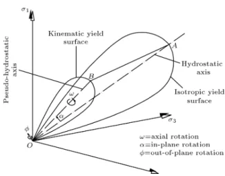
In the rotational kinematic hardening model, new rotated kinematic surface will be generated after a stress reversal, with its pseudo-hydrostatic axis passing through the stress reversal point, and then the direction of kinematic yield surface is determined. Note that the shape of kinematic yield surface is also the same as isotropic yield surface. The stress reversal point is dened as the tip of the new kinematic yield surface; in this way, size of the rotated kinematic yield surface is determined. Therefore, all information about the rotated kinematic yield surface is known.
Directions of the new kinematic yield surfaces were depicted in Figure 1. Rotational degrees of freedom were shown as angles corresponding to in-plane, out-of-plane and axial rotations. From the evolution rule of kinematic yield surface [34], the pseudo-hydrostatic axis will always rotate towards the
Figure 1. Rotation angles of kinematic yield surface in principal stress space.
hydrostatic axis; thus, the out-of-plane angle will always be zero. Lade et al. [34] pointed that kinematic surface would be free to rotate about its axis, this additional axial rotation should be taken into account; however. This may introduce complexity and numer-ical diculties of this model. Simply, it is suggested to x the kinematic surface against rotation about its own axis.
In accordance with the above discussion, the rotated principal stress could be expressed by principal stress in normal principal stress space as follows, where rotated principal stress is indicated by a star:
2 4
1
2
3
3 5 =
2 4 n
2
1(1 cos ) + cos
n1n2(1 cos ) n3sin
n1n3(1 cos ) + n2sin
n1n2(1 cos ) + n3sin
n2
2(1 cos ) + cos
n2n3(1 cos ) n1sin
n1n3(1 cos ) n2sin
n2n3(1 cos ) + n1sin
n2
3(1 cos ) + cos
3 5 2 412
3
3
5 ; (1) where is positive if anti clockwise, 1, 2, 3 are
principal stress in normal stress space;
1, 2, 3 are
principal stress in rotated stress space, and: n = (n1; n2; n3) =k A B
Ak kBk sin AB
=p (3B 2B; 1B 3B; 2B 1B)
(3B 2B)2+ (1B 3B)2+(2B 1B)2;(2)
is the unit normal vector of the plane in which kine-matic surface rotate; iB(i = 1; 2; 3) is the principal
stress of point B. Eq. (1) can be simply expressed as follows:
i = Tijj; (i; j = 1; 2; 3): (3)
Here, use Einstein convention of summation over re-peated indices, and:
T = 2 4 n
2
1(1 cos ) + cos
n1n2(1 cos ) n3sin
n1n3(1 cos ) + n2sin
n1n2(1 cos ) + n3sin
n2
2(1 cos ) + cos
n2n3(1 cos ) n1sin
n1n3(1 cos ) n2sin
n2n3(1 cos ) + n1sin
n2
3(1 cos ) + cos
3
5 ; (4) is the transform matrix.
2.2. General plasticity formula of rotated yield surface in principal stress space
Yield surface formula of the rotational kinematic hard-ening model could be generally written as:
F (I1; I2; I3) = f(H); (5)
or:
F (1; 2; 3) = f(H); (6)
where I1, I2, I3 are invariants of the stress tensor ij,
which can be dened by:
I1= x+ y+ z; (7)
I2=xyyx+ yzzy+ xzzx
(xy+ yz+ zx); (8)
I3=xyz+ xyyzzx+ yxzyxz
(xyzzy+ yzxxz+ zxyyx): (9)
In Eqs. (5) and (6), function f is the hardening rule with its parameter H, which usually relates to plastic strain.
In the rotated principal stress space, formula of the yield surface is the same as before with the stress values transformed into the rotated stress; thus, yield surface can be expressed as below:
F (I
1; I2; I3) = f(H); (10)
or: F (
1; 2; 3) = f(H); (11)
where I
1, I2, I3 and 1, 2, 3 are invariants and
principal stress in the rotated principal stress space, which can be calculated from Eqs. (1) to (4).
In numerical simulation, elastoplastic matrix is necessary; here the formula of the exibility matrix are given directly.
[Cep] = [De] 1+
@F
@ @G@
T
A ; (12)
where Deis the elastic matrix; @F@ is the normal vector
of the yield surface; @G
@ is the normal vector of the
potential surface; and A is related to hardening rule which is written as:
A = F0@H
@"p
T@G
@
; (13)
where F0 is the derivative of the F .
If the isotropic hardening yield surface is rotated, then its normal vector is:
@F @ =
@F (
1; 2; 3)
@ =
@F (
1; 2; 3)
@ 1
@ 1
@
+@F (1; 2; 3)
@ 2 @ 2 @ + @F (
1; 2; 3)
@ 3
@ 3
@(14): From Eq. (4), Eq. (14) becomes:
@F @ =T1j
@F (
1; 2; 3)
@ 1
@j
@
+ T2j@F (
1; 2; 3)
@ 2
@j
@
+ T3j@F (
1; 2; 3)
@ 3
@j
@: (15) Here, use Einstein convention of summation over re-peated indices.
In the principal stress space, = [1; 2; 3]T,
thus @1
@ = [1; 0; 0]T,@@2 = [0; 1; 0]T, @@3 = [0; 0; 1]T,
however, in numerical calculation components of stress are often used, i.e. = [x; y; z; xy; yz; zx]T,
therefore, it will be more complex to obtain the @i
@.
Here, the relation of the principal stress and stress components is introduced. Recall that the principal stresses are the three roots of the following equation:
3 I
12 I2 I3= 0;
I1= x+ y+ z; (16)
where:
I2=xyyx+ yzzy+ xzzx
(xy+ yz+ zx);
I3=xyz+ xyyzzx+ yxzyxz
(xyzzy+ yzxxz+ zxyyx):
Three roots of Eq. (16) indicates the relationship of principal stress and stress components in a explicit formula. According to the \root formula" of Eq. (16):
1= 2
q
J2
3 cos +I31
2= 2
q
J2
3 cos( 23) +I31
3= 2
q
J2
3 cos( +23) +I31
9 > > > > > > > = > > > > > > > ; ; (17a) where:
cos 3 = 3 p
3 2
J3
J32
2
; (17b)
J2= sxsy+ sysz+ szsx xy2 yz2 zx2 ; (17c)
J3=sxsysz+ 2xyyzzx sxyz2
syzx2 szxy2 : (17d)
Therefore:
@1
@ = 2 r
J2
3 sin @
@ + cos 1 p
3J2
@J2
@
+13@I@1; (17e)
@I1
@ =
1 1 1 0 0 0T; (17f)
and: @J2
@ =
sx sy sz 2sxy 2syz 2szxT; (17g)
@J3
@ =
sysz s2yz J32 szsx s2zx J32
sxsy s2xy J32 2(szxsyz szsxy)
2(sxyszx sxsyz) 2(syzsxy syszx)T;
(17h) @ @ = p 3 2
J32
2 @J@3 32J3J
1 2
2 @J@2
J3 2
s 1
3p3J3
2J32 2
2; (17i)
where sij is the deviatoric part of stress tensor.
Substituting Eqs. (17f) to (17i) into Eq. (17e), stress gradients of 1is obtained; similarly, derivatives
of the other two principal stresses are: @2
@ = 2 r
J2
3 sin
2 3
@ @
+ cos
23
1 p
3J2
@J2
@ + 1 3
@I1
@; (17j) @3
@ = 2 r
J2
3 sin
+23
@ @
+ cos
+ 23
1 p
3J2
@J2
@ + 1 3
@I1
@: (17k) The normal vector of potential surface @G
@ can be
obtained from Eqs. (14) to (17) with plastic potential function G substituting for F . Hardening rule of the rotated kinematic yield surface Eq. (13) will be discussed in the next section.
2.3. Brief description of Lade-Kim model The above-mentioned general plasticity formula could be used within the framework of any constitutive model. This paper adopted the Lade-Kim model [35-37] as an example. The following derivations are nec-essary for us before discussing its kinematic hardening. The total strain increments are divided into elastic and plastic component such that:
d"ij= d"eij+ d"pij: (18)
The strain increments are calculated separately; the elastic strains by Hooke's law and the plastic strain by the plasticity theory.
Elastic behavior
Elastic modulus is expressed in the following form, and the Poisson's ratio is assumed to be constant:
E = M:pa
3
pa
; (19)
in which pa is atmospheric pressure, 3 is the third
principal stress, M and are material parameters. Yield surface and stress level
The yield surface describes the contours of equal total plastic work; the total plastic work serves as the hardening parameter. The isotropic yield function is dened as:
F =
1I 3 1
I3
I2 1
I2
I1
pa
h
eq; (20)
in which:
q = 1 (1 ):S:S : (21) Stress level S is dened as:
S = 1
1
I3
1
I3 27
I1
pa
m
: (22)
Hardening rule is dened as:
F =
1 D
1 Wp
pa
1
; (23)
in which: D = c
(27 1+ 3); (24)
=hp; (25)
1= 0:00155:m 1:27; (26)
where h, , c, p, m, 1are material parameters.
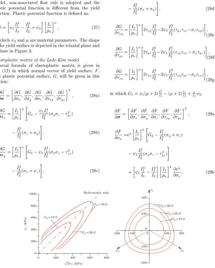
The shape of the yield surfaces are depicted in the triaxial plane and plane in Figure 2. Material parameters are obtained from the tests of Loose Santa Monica beach sand.
Figure 2. Yield surfaces shown in principal stress space: (a) Yield surface in triaxial plane; and (b) yield surface in plane (I1= 500 kPa).
Plastic potential surface
The direction of the plastic strain increment is deter-mined by plastic potential surface. In the Lade-Kim model, non-associated ow rule is adopted and the plastic potential function is dierent from the yield function. Plastic potential function is dened as:
G = 1I 3 1 I3 I2 1
I2 + 2
I1
pa
; (27)
in which 2and are material parameters. The shape
of the yield surface is depicted in the triaxial plane and plane in Figure 3.
Elastoplastic matrix of the Lade-Kim model
General formula of elastoplastic matrix is given in Eq. (12) in which normal vector of yield surface, F , and plastic potential surface, G, will be given in this section:
@G @ =
@G @x;
@G @y;
@G @z;
@G @xy;
@G @yz
T
; (28a)
@G @x =
I1
pa
"
G1 1I 3 1
I2
3 (yz 2 yz)
I2 1
I2
2(z+ y)
#
; (28b)
@G @y =
I1
pa
"
G1 1I 3 1
I2
3(xz 2 zx)
I2 1
I2
2(x+ z)
#
; (28c)
@G @z =
I1
pa
"
G1 1I 3 1
I2
3(xy 2 xy)
I2 1
I2
2(x+ y)
#
; (28d)
@G @xy=
I1
pa
2xyI 2 1
I2 2 2 1
I3 1
I2
3(yzzx zxy)
; (28e)
@G @yz=
I1
pa
2yzI 2 1
I2 2 2 1
I3 1
I2
3(xyzx xyz)
; (28f)
@G @zx=
I1
pa
2zxI
2 1
I2 2 2 1
I3 1
I2
3(xyyz yzx)
; (28g)
in which G1= 1( + 3)I
2 1
I3 ( + 2)
I1
I2 +
I1 2.
@F @ =
@F @x;
@F @y;
@F @z;
@F @xy;
@F @yz
T
; (29a)
@F @x =e
qI1
pa
h"
G2 I 2 1
I2
2(y+ z)
1I 3 1
I2
3(yz 2 yz) # + 1I 3 1 I3 I2 1 I2 I1 pa h @eq
@x; (29b)
Figure 3. Plastic potential surfaces shown in principal stress space: (a) Plastic potential surface in triaxial plane; and (b) plastic potential surface in plane (I1= 500 kPa).
@F @y =e
qI1
pa
h" G2 I
2 1
I2
2(x+ z)
1I 3 1
I2
3(xz 2 zx) # + 1I 3 1 I3 I2 1 I2 I1 pa
h @eq
@y; (29c)
@F @z =e
q
I1
pa
h" G2 I
2 1
I2
2(x+ y)
1I 3 1
I2
3(xy 2 xy) # + 1I 3 1 I3 I2 1 I2 I1 pa
h @eq
@z; (29d)
@F @xy =e
qI1
pa
h
2II122
2xy 2 1I13
I2
3 (yzzx zxy)
+ 1I 3 1 I3 I2 1 I2 I1 pa h @eq
@xy; (29e)
@F @yz =e
qI1
pa
h
2I12
I2 2yz 2
1I13
I2
3 (xyzx xyz)
+ 1I 3 1 I3 I2 1 I2 I1 pa
h @eq
@yz; (29f)
@F @zx =e
q
I1
pa
h 2II122
2zx 2 1I13
I2
3 (xyyz yzx)
+ 1I 3 1 I3 I2 1 I2 I1 pa
h @eq
@xz; (29g)
in which: G2= 1I
2 1
I3(h + 3)
I1
I2(2 + h); (29h)
@eq
@x =e
q
(1 (1 )S)2
I1
pa
m( m I11
I3
1
I3 27
+ 3I12
1I3
I3 1
I2
31(yz 2 yz)
)
; (29i)
@eq
@y =e
q
(1 (1 )S)2
I1
pa
m( m
1I1
I3
1
I3 27
+ 3I12
1I3
I3 1
I2
31(xz 2 zx
)
; (29j)
@eq
@z =e
q
(1 (1 )S)2
I1
pa
m( m 1I1
I3
1
I3 27
+ 3I12
1I3
I3 1
I2
31(xy 2 xy)
)
; (29k)
@eq
@xy =e
q
(1 (1 )S)2
I1 pa m I3 1 I2
31(2yzzx 2zxy)
; (29l)
@eq
@yz =e
q
(1 (1 )S)2
I1 pa m I3 1 I2
31(2xyzx 2xyz)
; (29m)
@eq
@zx =e
q
(1 (1 )S)2
I1 pa m I3 1 I2
31(2xyyz 2yzx)
: (29n) In the Lade-Kim model, plastic work is used as hard-ening parameter, then Eq. (13) becomes:
A = 1[Dpa] 1W 1
p fgT
@G @
: (30) Thus, elastoplastic matrix could be obtained, where Wp
is the plastic work.
3. Evolution rules of the yield surfaces and plastic potential surfaces
3.1. Generation of the new kinematic yield surface and its evolution rule
Under the primary monotonic loading, only the isotropic hardening yield surface is valid. Once any stress reversal leads to unloading within the yield surface, a new kinematic surface would generate with its tip at the stress reversal point. In this manner, the original kinematic yield surface forms. The space enclosed both by the isotropic yield surface and the kinematic surface is totally elastic. Any stress reversals reaching the kinematic yield surface will activate the kinematic yield surface, and plastic strain will occur. The kinematic yield surface evolution law obeys two constraints:
1. Kinematic surface tip moves towards tip of the isotropic hardening surface on a straight [31,32] or parabolic [34] line.
2. The current stress state must be on the kinematic yield surface.
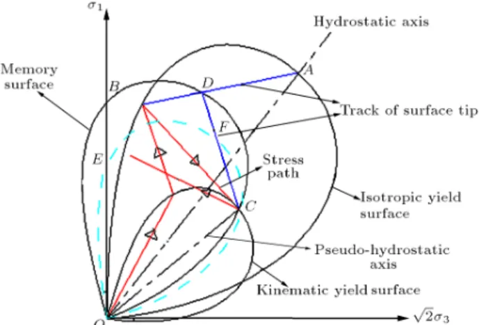
Figure 4. Generation and evolution of the kinematic yield surface during the rst time stress reversal in triaxial plane.
As shown in Figure 4, in a new kinematic yield surface generated with its pseudo-hydraulic axis OB, point B is the stress reversal point. Surface tip moves along BA towards point A. When the current stress is at point C, then kinematic yield surface rotates with its tip point D, which was sketched in Figure 4 with dashed line. Using Eqs. (1)-(2), principal stress in the normal stress space can be converted into rotated principal stress and angle is dened as:
cos =kA:D
Ak : kDk; (31)
where Aand D are stress vector of points A and D
in principal stress space, e.g. A= [1A; 2A; 3A]T.
If the current stress continues in a xed direction and nally reaches the isotropic yield surface, then the isotropic yield surface is activated, and the kinematic yield surface merges into the isotropic yield surface; all past history eects due to kinematic hardening are wiped out.
Note that the location of the kinematic yield surface is not decided by hardening rule, but by the two constraints mentioned above. Assume that point D moves on the straight line AB, then coordinates of point D can be shown as:
2 41D2D
3D
3 5 =
2 41B2B
3B
3 5 +
2
41B2B 1A2A 3B 3A
3
5 ; (32) where is a multiplier within [0,1]. Points D and C are on the same yield surface (dashed line in Figure 4), thus in the rotated principal stress space:
F (
1C; 2C; 3C ) = F (1D ; 2D; 3D): (33)
Recall that
C can be expressed by A, B, C and
cos according to Eqs. (1)-(2); in turn, cos can be expressed by , A, B according to Eqs. (31)-(32).
Similarly,
D can be expressed by A, B and
according to Eqs. (1), (2), (31) and (32). Thus Eq. (33) becomes:
F (A; B; C; ) = F (A; B; ): (34)
Eq. (34) forms the governing equation dening the motion of the kinematic yield surface; at any load step, the only unknown is , which can be determined numerically by several iterations.
3.2. Generation and elimination of the kinematic yield surface during multiple times of stress reversals
In the above section, generation and evolution of the kinematic yield surface during the rst time stress reversal was discussed. In Figure 4, if another stress reversal occurs at point C, then new kinematic yield surface will generate with OC as its pseudo-hydrostatic axis, and the current kinematic yield surface (dashed line in Figure 4) becomes the \Memory surface", as shown in Figure 5. The kinematic yield surface generated at the rst time was forgotten. It means that in the process of yield surface evolution, yield surface tip rst moves on line CD towards point D until the stress reaches \memory surface". Once the current stress point reaches \memory surface", then the current kinematic yield surface merges into the \memory surface", and \Memory surface" will be activated. After that, \memory surface" tip moves on line DA towards point A. Governing equation of yield surface motion was the same as Eq. (34), except that trace of kinematic yield surface tip changed from path AB to bilinear C D A.
If a new stress reversal occurs at point E, again in Figure 5, then another new kinematic yield surface will be created with its pseudo-hydrostatic axis OE, as shown in Figure 6. In this gure the current kinematic surface is now recorded as the new memory surface. It is easy to follow the same logic like the initial stress reversal that kinematic yield surface tip moves on multi-segment line E F D A, i.e. rstly, the yield surface tip moves on line EF , and when the stress reaches the new memory surface, the new
Figure 5. Generation and evolution of the kinematic yield surface during the second stress reversal in triaxial plane.
Figure 6. Generation and evolution of the kinematic yield surface during the third stress reversal in triaxial plane.
memory surface is activated, then the kinematic yield surface tip again moves on bilinear F D A just like in Figure 5. However, in this manner, during large number of stress reversals, a large number of memory surfaces will be recorded. This leads to more complexity of this model. Lade et al. [31,32] indicated that \Experimental observations show that soil tends to forget previous yielding mechanisms after sucient yielding is activated by the latest surface; it was found to be appropriate to remember only one surface prior to the current kinematic surface, this surface will be referred to as memory surface", therefore, in Figure 6, once the stress reverses at point E, the kinematic yield surface prior to the current yield surface is recorded as memory surface; the old memory surface is eliminated so that it has no eect on the soils behaviors. Therefore, the kinematic yield surface tip moves on the bilinear E F A instead of E F D A. Memory surface concept was also used by Wang et al. [8] and Wang [38] in their bounding surface model when dening the mapping rule.
With the concept of the memory mechanism, at most three surfaces (i.e. isotropic yield surface, memory surface and kinematic yield surface) are to be recorded. New stress reversals results in forming new kinematic yield surface and memory surface, eliminat-ing the old memory surface. In this process, position of the kinematic yield surface is determined according to Eq. (34) with stress points A, B and C which refer to isotropic yield surface tip (for three surfaces) or memory surface tip (for two surfaces), stress reversal point and current stress point, separately.
3.3. Evolution of the plastic potential and the hardening rule
Directions of the plastic strain are determined by plastic potential surface, if the soils obey the associated ow rule, yield and potential surface are consistent, so that their evolution rules are the same. When a non-associated ow rule is adopted, yield surface and plastic potential surface are separated. Lade and Inel [31]
assumed that the plastic potential surface is always attached to the kinematic yield surface, and moves along and expands or shrinks with yield surface. This assumption was in accordance with the experimentally observed behavior by Lade and Boonyachut [39]. Under this assumption, the rotation angles of the plastic potential are the same as that of kinematic yield surface.
Hardening rule of the yield surface is assumed to be universally valid for both isotropic and kinematic hardening. If the plastic work is as the hardening index, for any load step, the increment of the plastic work is determined by the slope of the work hardening curve:
Wp=FF0(W
p); (35)
where F is the yield surface in Eq. (11), F is the increment of F in the process of evolution that can be obtained from evolution rule of kinematic yield surface and F0(W
p) is the derivation of F (Wp).
When Lade-Kim model is applied with the rota-tional kinematic yield concept, Eq. (34) becomes:
1I 3 1C
I 3C
I2 1C
I 2C
I 1C
pa
h
eq= (27 1+ 3)
I1D
pa
h ; (36) where point C is the current stress point and point D is the kinematic yield surface tip; values in rotated principal stress space are indicated by star.
Hardening rule of Eq. (13) becomes:
Wp=h F 1 Dpa
i1
W1 1
p
: (37)
4. Logical procedures of model implement 4.1. Logical procedures design
According to the discussion in Section 3, we know that kinematic hardening model is more complex than conventional elastoplastic model in determining the load mode of soil state. A proper logical procedures design is especially important in model implement. This paper designs the new logical procedures as shown in Figure 7, in which NF is the current number of yield surfaces, M is used to indicate the state of soil element at the previous load step (e.g. if soil element yield M = 1 otherwise M = 0), (fmax)i is the maximum
history stress of yield surface i in the corresponding stress space.
4.2. Verication
Rotational kinematic hardening model within the framework of Lade-Kim model was validated with test results of Loose Santa Monica beach sand. Source
Figure 7. Flowchart of implement of the kinematic hardening model.
Figure 8. Comparison of test results and model prediction of Loose Santa Monica beach sand during stress reversals (3= 117:7 kPa).
codes of rotational kinematic hardening model in tri-axial state (written in Fortran 95) were listed in the Appendix. Comparisons of measured and predicted stress-strain curves were shown in Figure 8. Material properties for Loose Santa Monica beach sand are shown in Table 1.
According to Figure 8 the predictions of rotational
kinematic hardening model matched the test results well. In Figure 8(a), a closed hysteresis loop can be modeled during loading and unloading, which was consistent with the test phenomena. In Figures 8(b) and (c), there are two and three stress reversals, sepa-rately; model predicts match the experiment behavior with good accuracy. Logical procedures developed by
Table 1. Material properties for Loose Santa Monica beach sand.
Material parameter M a m 1 C p 2 h
this paper have been successfully used in implementing the kinematic hardening model, obeying the evolution rules of yield surfaces.
5. Conclusions
In this research, a rotational kinematic hardening model has been studied in detail; this model is used to simulate large stress reversals of soil, which is also a fundamental research for soil dynamics. This model simulates the stress reversals by rotating and intersecting of the isotropic hardening yield surface, therefore, no additional model parameter is introduced. On the other hand, this model does not need to obey the tangency conditions, thus it can be widely used.
The main conclusions of the research are as follows:
1. A general plasticity formula of rotated isotropic hardening model in principal stress space was given, that can be generally used in rotational kinematic yield surface.
2. Evolution rule of the yield surface and plastic potential surface were elaborated. This includes, generation of the new kinematic yield surface and memory surface, rotation of the kinematic yield surface, determination of the surface's location in the process of loading, activation or elimination of the memory surface, etc. It is assumed that the plastic potential surface is always attached to yield surface.
3. New logical steps to determine loading mode of soil were designed and source codes were listed in the Appendix. These logical procedures were successfully used within the framework of the Lade-Kim; tests data of the soils that experienced stress reversal were compared with the model predictions. Model predictions match the test results with good accuracy.
Acknowledgements
This research is funded by National scientic and technological support plan subject of China (2009BAK56B02, 2009BAK56B04). The authors are grateful for this support.
References
1. Roscoe, K.H. Schoeld, A.N. and Wroth, C.P. \On the yielding of soils", Geotechnique, 8(1), pp. 22-52 (1958).
2. Lade, P.V. \Elasto-plastic stress-strain theory for co-hesionless soil with curved yield surfaces", Int. J. Solids Struct, 13(11), pp. 1019-1035 (1977).
3. Shen, Z.J. \Elasto-plastic analysis of consolidation and deformation of soft ground", Science Sinica (A series), XXIX(2), pp. 210-224 (1986).
4. Nakai, T. \An isotropic hardening elastoplastic model for sand considering the stress path dependency in three-dimensional stresses", Soils and Foundations, 29(1), pp. 119-137 (1989).
5. Alonso, E.E., Gens, A. and Josa, A. \A constitutive model for partially saturated soils", Geotechnique, 40(3), pp. 405-430 (1990).
6. Wichtmann, T. and Triantafyllidis, Th. \Inuence of a cyclic and dynamic loading history on dynamic properties of dry sand. Part I: Cyclic and dynamic torsional prestraining", Soil. Dyn. Earthq. Eng., 24(2), pp. 127-147 (2004).
7. Keshavarz, A., Jahanandish, M. and Ghahramani, A. \Seismic bearing capacity analysis of reinforced soils by the method of stress characteristics", Sci. Iran., 35(C2), pp. 185-197 (2011).
8. Wang, Z.L., Dafalias, Y.F. and Shen, C.K. \Bounding surface hypoplasticity model for sand", J. Eng. Mech. ASCE, 116(5), pp. 983-1001 (1990).
9. Niemunis, A., Wichtmann, T. and Triantafyllidis, Th. \A high-cycle accumulation model for sand", Comput. Geotech., 32(4), pp. 245-263 (2005).
10. Dafalias, Y.F., Kourousis, K.I. and Saridisa, G.J. \Multiplicative AF kinematic hardening in plasticity", Int. J. Solids Struct., 45(10), pp. 2861-2880 (2008).
11. Dafalias, Y.F. and Popov, E.P. \A model of nonlin-early hardening materials for complex loading", Acta Mechanica, 21(3), pp. 173-192 (1975).
12. Dafalias, Y.F. and Popov, E.P. \Plastic internal vari-ables formalism of cyclic plasticity", Journal of Applied Mechanics, 43(4), pp. 645-651 (1976).
13. Dafalias, Y.F. and Popov, E.P. \Cyclic loading for materials with a vanishing elastic region", Nuclear Engineering and Design, 41(2), pp. 293-302 (1977).
14. Dafalias, Y.F. \Bounding surface plasticity. I: Mathe-matical foundation and hypoplasticity", J. Eng. Mech. ASCE, 112(9), pp. 966-987 (1986a).
15. Dafalias, Y.F. \Bounding surface plasticity. II: Ap-plication to isotropic cohesive soils", J. Eng. Mech. ASCE, 112(12), pp. 1263-1291 (1986b).
16. Hashiguchi, K. \Plastic constitutive equation of gran-ular material", Proc. US-Japan seminar Continuum Mech. Statistical Approaches in Mech. Gran. Materi-als., Sendai, p. 321 (1978).
17. Hashiguchi, K. \Constitutive equations of granular media with an anisotropic hardening", Proc. 3rd Int. Conf. Numer. Mech. Geomech. Aachen, p. 435 (1979).
18. Hashiguchi, K. \Constitutive equations of elastoplastic materials with elastic-plastic transition", Journal of Applied Mechanics, 47(2), pp. 266-272 (1980).
19. Hashiguchi, K. \Constitutive equations of elastoplas-tic materials with anisotropic hardening and elaselastoplas-tic- elastic-plastic transition", Journal of Applied Mechanics, 48(2), pp. 297-301 (1981).
20. Hashiguchi, K. \A mathematical modication of two surface model formulation in plasticity", Int. J. Solids Struct., 24(10), pp. 987-1001 (1988).
21. Hashiguchi, K. \Subloading surface model in uncon-ventional plasticity", Int. J. Solids Struct., 25(8), pp. 917-945 (1989).
22. Hashiguchi, K. and Chen, Z.-P. \Elastoplastic consti-tutive equation of soils with the subloading surface and the rotational hardening", Int. J. Numer. Meth. Eng., 22(3), pp. 197-227 (1998).
23. Hashiguchi, K., Ozaki, S. and Okayasu, T. \Unconven-tional friction theory based on the subloading surface concept", Int. J. Solids Struct., 42(5-6), pp. 1705-1727 (2005a).
24. Hashiguchi, K. \Generalized plastic ow rule", Int. J. Plasticity, 21(2), pp. 321-351 (2005).
25. Hashiguchia, K. and Ozakib, S. \Constitutive equation for friction with transition from static to kinetic fric-tion and recovery of static fricfric-tion", Int. J. Plasticity, 24(11), pp. 2102-2124 (2005b).
26. Andrianopoulosa, K.I., Papadimitrioub, A.G. and Bouckovalas, G.D. \Bounding surface plasticity model for the seismic liquefaction analysis of geostructures", Soil. Dyn. Earthq. Eng., 30(30), pp. 895-911 (2010).
27. Suebsuka, J., Horpibulsuk, S. and Liu, M.D. \A critical state model for overconsolidated structured clays", Comput. Geotech., 38(5), pp. 648-658 (2011).
28. Nakai, T. and Hinokio, M. \A simple elastoplastic model for normally and over consolidated soils with unied material parameters", Soils and Foundations, 44(2), pp. 53-70 (2004).
29. Yao, Y.P., Hou, W. and Zhou, A.N. \UH model: Three-dimensional unied hardening model for over-consolidated clays", Geotechnique, 59(5), pp. 1-19 (2007).
30. Pedrosoa, D.M. and Farias, M.M. \Extended barcelona basic model for unsaturated soils under cyclic load-ings", Comput. Geotech., 38(5), pp. 731-740 (2011).
31. Lade, P.V. and Inel, S. \Rotational kinematic harden-ing model for sand. Part I: Concept of rotatharden-ing yield and plastic potential surfaces", Comput. Geotech., 21(3), pp. 183-216 (1997a).
32. Inel, S. and Lade, P.V. \Rotational kinematic hard-ening model for sand. Part II: Characteristic work hardening law and predictions", Comput. Geotech., 21(3), pp. 217-234 (1997b).
33. Yao, Y.P., Wan, Z. and Qin, Z.H. \Dynamic UH models for sands and its application in FEM", Chinese Journal of Theoretical and Applied Mechanics, 44(1), pp. 132-139 (2012). (In Chinese)
34. Lade, P.V., Gutta, S.K. and Yamamuro, J. \A. Kine-matic hardening predictions of large stress-reversals in 3-D test on loose sand", Comput. Geotech., 36(8), pp. 1285-1297 (2009).
35. Lade, P.V. and Kim, M.K. \Single hardening constitu-tive model for frictional materials: II. Yield criterion and plastic work contours", Comput. Geotech., 6(1), pp. 13-29 (1988b).
36. Lade, P.V. and Kim, M.K. \Single hardening consti-tutive model for frictional materials: III. Comparisons with experimental data", Comput. Geotech., 6(1), pp. 31-47 (1988c).
37. Kim, M.K. and Lade, P.V. \Single hardening con-stitutive model for frictional materials: I. Plastic potential function", Comput. Geotech., 5(4), pp. 307-324 (1988a).
38. Wang, Z.L. \bounding surface plasticity model for granular soils and its applications", Ph.D. Thesis, University of California, Davis (1990).
39. Lade, P.V., and Boonyachut, S. \large stress reversals in triaxial tests on sand", 4th Int. Conf. Numer. Mech. Geomech., Edmonton, pp. 171-181 (1982).
Appendix
Source codes of rotational kinematic hardening model in triaxial test state
For the limitation of the publi-cation, here is the list of the main part of the program readers can get the full program at URL: http://blog.sina.com.cn/s/ blog a94cb93e0101c4lz.html
Notations
1. Subroutines:
LadeKim Calculate plastic matrix of rotational kinematic hardening within framework of Lade-Kim model
JUDGE Determinate which yield surface yields or stress reversal occurs
PRO Generate new kinematic yield surface, once the stress reversal occurs
PFLOW Calculate the normal vector of yield surface or potential surface in a general formulation
LOCATION Specify the location of the kinematic yield surface during loading according to evolution rule
ROHDEN Hardening of the kinematic yield surface
ZREAL Internal function to nd the solution of function F
F Function that describes the evolution rule
2. Arrays:
PEAK(*) Surface tip of the kinematic yield surface in normal principal stress space AGL(*) Cosine of the rotation angle of each
yield surface
TP(*,*) Stress point dened the movement of the kinematic yield surface
STS(*) Total stress of each load step ZZS(*) Principal stress of each load step FAX(*) Maximum stress in loading history TURP(*,*) Surface tip of the kinematic yield
surface in rotated principal stress space STL(*) Stress components of the last load step CP(*,*) Plastic matrix
TT(*,*) Matrix to transform the current stress to rotated principal stress
DM(*,*) Elastoplastic matrix
FA(*) Normal vector of yield surface GA(*) Normal vector of potential surface
3. Note that when call the internal function ZREAL, proper guess value should be given.
SUBROUTINE LadeKim (STS, ZZS, STS0, ZZS0, WP, & WP0, JP, DM, CP, FAX, TURP, MEM, TP, PLW, AGL, MES, NF, STL, PEAK, IP)
USE IMSL
COMMON/GROUP4/CTR(13, 1)
DIMENSION STS(8), STS0(8), ZZS0(3), ZZS(3) DIMENSION GA(6), FA(6), CP(6, 6), CM(6, 6) DIMENSION DM(6, 6), FAX(5)
DIMENSION TT(3, 3), TURP(6, 3), MEM(6)
DIMENSION TP(6, 20), PLW(3), AGL(3), STL(6), PEAK(6)
AA=0.0 PA=100. MES=0 DO I=1, 6 DO J=1, 6 CP(I, J)=0.0 ENDDO ENDDO
S1=ZZS0(1)+ZZS0(2)+ZZS0(3)
S2=-(ZZS0(1)*ZZS0(2)+ZZS0(2)*ZZS0(3) +ZZS0(1)*ZZS0(3))
S3=ZZS0(1)*ZZS0(2)*ZZS0(3) SX=-STS0(1)
SY=-STS0(2) SZ=-STS0(3)
PSA1=0.00155*CTR(6, 1)**(-1.27) RP=CTR(11, 1)/CTR(12, 1)
DS=CTR(10, 1)/((27.0*PSA1+3.0)**RP) DO ID=1, NF
COSA=AGL(ID)
CALL JUDGE (STS , ZZS0, STS0, PS, CP, FAX, GA, COSA, ID, MES, TURP, JP, PEAK)
IF(MES.NE.0) THEN DO I=MES+1, 3 FAX(I)=0.1
PLW(I)=1.0e-2 AGL(I)=1.0 TP(1, I-1)=0.0 TP(2, I-1)=0.0 TP(3, I-1)=0.0 TURP(1, I-1)=0.0 TURP(2, I-1)=0.0 TURP(3, I-1)=0.0 NF=MES
ENDDO ENDIF
IF(MES.NE.0) EXIT ENDDO
IF(MES.NE.0.AND.JP.EQ.2) THEN MEM(1)=MES
ENDIF
IF(MES.EQ.0.AND.JP.EQ.2) THEN IF(MEM(1).EQ.1) THEN
IID=MEM(1) TP(1, IID)=STL(1) TP(2, IID)=STL(2) TP(3, IID)=STL(3)
CALL PRO(SX, SY, SZ, FAX, IID, COSA, PLW) AGL(IID+1)=COSA
NF=NF+1
ELSEIF(MEM(1).EQ.2) THEN IID=MEM(1)
TP(1, IID-1)=PEAK(1) TP(2, IID-1)=PEAK(2) TP(3, IID-1)=PEAK(3) TP(1, IID)=STL(1) TP(2, IID)=STL(2) TP(3, IID)=STL(3)
CALL PRO(SX, SY, SZ, FAX, IID, COSA, PLW) AGL(IID+1)=COSA
NF=NF+1
ELSEIF(MEM(1).EQ.3) THEN FAX(2)=FAX(3)
PLW(2)=PLW(3) AGL(2)=AGL(3) TP(1, 1)=PEAK(1) TP(2, 1)=PEAK(2) TP(3, 1)=PEAK(3) TP(1, 2)=STL(1) TP(2, 2)=STL(2) TP(3, 2)=STL(3) PLW(3)=0.01 IID=MEM(1) FAX(3)=0.1
CALL PRO(SX, SY, SZ, FAX, IID, COSA, PLW) AGL(3)=COSA
NF=NF+1 ENDIF ENDIF
IF(MES.EQ.0.AND.JP.EQ.2) THEN MEM(1)=0
ENDIF
IF(MES.EQ.0) GOTO 200 IF(MES.EQ.1) THEN COSA=AGL(1)
CALL PFLOW (STS, ZZS0, STS0, PS, CP, FAX, GA, COSA, MES, PEAK, f2)
DO I=1, 6
AA=AA-STS0(I)*GA(I) ENDDO
AA=AA*1.0/RP*(1.0/DS/PA)**(1.0/RP) *WP0**(1.0/RP-1.0)
ELSE
CALL LOCATION (STS, ZZS, STS0, ZZS0, & CP, FAX, TURP, MEM, TP, PLW, MES, COSA, AGL, JP, PEAK, IP)
IF(JP.EQ.2) AGL(MES)=COSA
CALL PFLOW (STS, ZZS0, STS0, PS, CP, FAX, GA, COSA, MES, PEAK, f2)
DO I=1, 6
AA=AA-STS0(I)*GA(I) ENDDO
CALL ROHDEN(PLW, AA, STS, ZZS0, STS0, PS, CP, FAX, GA, COSA, MES, JP, f2) ENDIF
DO I=1, 6 DO J=1, 6
CP(I, J)=CP(I, J)/AA ENDDO
ENDDO 200 CONTINUE
WRITE(16, *) AA CM=.I.DM DO I=1, 6
DO J=1, 6
CM(I, J)=CM(I, J)+CP(I, J) ENDDO
ENDDO DM=.I.CM END
Biographies
Kuangmin Wei was born in 1985 in Gansu province of China, PhD of Hohai University. He is inter-ested in constitutive model and elastoplastic theories in geotechnical Engineering. In recent years, he studied elastoplastic models (e.g. bounding surface model, rotational hardening model, generalized plas-ticity model, etc.), to predict mechanical behaviors of soil under complex loading conditions. He has published several articles in journals, books and pro-ceedings.
Sheng Zhu was born in 1965 in Hunan province of China. He is the Professor of hydraulic structures in Hohai University, Institute of Hydraulic Structures. His research interests include: Mechanical proper-ties of coarse grained soils under complex loadings, time-dependent properties of the corpse grained soils, constitutive model of soils, seismic analysis of rock-ll dam, etc. Many results are successfurock-lly used in dam construction. His group is also involved in the construction of Shuibuya rock-ll dam, which is the highest Concrete-Faced Rock-ll Dam in the world. He has published more than 40 articles in journals, books, and proceedings.