Project resource investment problem under progress payment
model
3
, Aria Shahsavar
* 2
, Amir Abbas Najafi
1
Elham Merrikhi
1Research School of Management, Australian National University, Canberra, Australia 2Faculty of Industrial Engineering, K.N. Toosi University of Technology, Tehran, Iran 3Faculty of Industrial and Mechanical Engineering, Islamic Azad University, Qazvin Branch, Qazvin,
Iran
[email protected], [email protected], [email protected]
Abstract
As a general branch of project scheduling problems, resource investment problem (RIP) considers resource availabilities as decision variables to determine a level of employed resources minimizing the costs of the project. In addition to costs (cash outflows), researchers in the later extensions of the RIP took payments (cash inflows) received from clients into account and used the net present value (NPV) of project cash flows as a financial criterion evaluating the profitability of the project. A striking point in a financial view of the project scheduling is how cash inflows are paid by client. There are different payment models in the literature of which progress payment is highly common in practice. In this paper, resource investment problem with maximization of the NPV under progress payment model is investigated. A new mathematical model is developed for the problem and then two metaheuristic algorithms based on the genetic algorithm (GA) and simulated annealing algorithm (SA) is suggested. The experimental results of algorithms are compared with some near optimal solutions derived from LINGO software. The comparisons show that the results of GA are more reliable than SA.
Keywords: Project scheduling, Resource investment, Net present value, Progress payment.
1-Introduction and Literature review
Introduced in the late 1950s, the project scheduling problem has been widely considered by researchers in different views resulting in different branches. One of the well-researched branches is resource leveling problem (RLP) which aims at minimization of the variation of the resource requirements during the project life cycle (Ahuja, 1976). The resource constrained project scheduling problem (Blazewicz et al., 1983) is the most well-known and researched model in project scheduling which minimizes the make-span of a project at scarce resource situation. The Resource investment problem is another well-known branch introduced by Mohring (1984) in which the resource availability is considered as decision variable with aim of finding a schedule for activities together with the availability of resources minimizing the renewable resource costs of the project.
*Corresponding author
ISSN: 1735-8272, Copyright c 2018 JISE. All rights reserved
Journal of Industrial and Systems Engineering
Vol. 11, No. 3, pp. 84-101
Summer (July) 2018
Demeulemeester (1995) presented an exact algorithm for RIP based on a branch and bound method previously designed for resource constrained project scheduling problem. Zimmermann and Engelhardt (1998) developed another branch and bound procedure for RIP under generalized precedence relations (RIP/max). Nübel (1999) suggested another method for RIP/max with the help of fictitious resource capacities and the resolution of resulting resource conflicts. Later on, Nübel (2001) developed a depth-first branch-and-bound method for solving a generalized RIP/max. In addition, Drexel and Kimms (2001) employed Lagrangian relaxation for finding the lower and upper bound for the RIP. As for metaheuristic procedures, Yamashita et al. (2006) proposed a scatter search, Shadrokh and Kianfar (2007) suggested a GA where the penalty would be forced to the project if the tardiness is met, and Ranjbar et al. (2008) introduced a path relinking and genetic algorithm procedure to tackle the RIP. Sabzehparvar et al. (2008) proposed a mathematical model for the RIP with multi-execution activities. Rodrigues and Yamashita (2010) proposed a hybrid method in which a heuristic algorithm feeds a branching approach to find optimal solution. Afshar-Nadjafi (2014) developed a mixed integer programming formulation for the multi-mode RIP wherein resources have recruitment and release dates. They also proposed a simulated annealing problem. Qi et al. (2015) designed a hybrid particle swarm optimization and scatter search to find satisfying solutions for the multi-mode RIP. Shahsavar et al. (2016) studied an integration of RIP and material ordering and proposed three hybrid metaheuristics. Javanmard et al. (2016) added multi-skilled view to the RIP to minimize total cost of recruiting different levels of skills. Two metaheuristic algorithms with calibrated parameters were also designed.
The integration of project scheduling and financial indexes was firstly done by Russel (1970) who considered the maximization of the project’s cash flows as the objective. Grinold (1972) presented an algorithm to evaluate the exact trade-off between net present value and project completion time. Smith-Daniels and Aquilano (1987) considered Russell’s work in the presence of the time for occurring positive and negative cash flows of the project. They illustrated an example in which the NPV is maximized by scheduling all non-critical activities with negative cash flow at the latest possible time and scheduling activities with positive cash flows at the earliest possible time. Elmaghraby and Herroelen (1990) developed an approach for solving max-NPV problems without resource constraints in an AOA network and fixed cash flow. Later, Herroelen and Gallens (1993) showed more computational experience for the work of Elmaghraby and Herroelen (1990). Etgar et al. (1996) formulated a problem of time-dependent cash flows to maximize the NPV. In their model, the bonus and penalty for the early and late events were considered. In addition, the costs were assumed to be changing over time. Shtub and Etgar (1997) proposed a branch and bound algorithm for the problem of NPV maximization of time-dependent cash flows in project scheduling. Doersch and Patterson (1997) presented a zero-one mathematical model in the condition of limited budget. Vanhoucke et al. (1999) considered the non-increasing linear cash flows in an AON network without resources constraints and in a condition where negative cash flows are occurred at the end of activities. They suggested a backtracking search algorithm in which the entire project activities are scheduled in the earliest possible time and then identified the series of activities that can maximize NPV by a backtracking search and then pushes the activities forwards as much as permitted. Etgar and Shtub (1999) assumed that the cash flows are linear functions of the events realization time and developed an optimal solution for the problem. Najafi and Niaki (2006) introduced the integration of RIP and max-NPV and proposed a GA for the problem. Later on, Najafi et al. (2009) studied RIP/max under max-NPV and presented a parameter-tuned GA. Najafi and Azimi (2009) permitted the problem to be tardy with penalty and proposed heuristic approaches. Shahsavar et al. (2011) assessed RIP/max with discounted cash flows under inflationary conditions where earliness and tardiness is also permitted with a bonus and penalty.
An essential part of real projects that is stipulated in the contracts is how the contractor receives the payments or cash outflows from the client. In the literature, there are four types of payment models. In Lump-sum payment (LSP) type, the whole payment is received at the completion time of the project. In the payments at event occurrence (PEO) type, some events of the project are predetermined for receiving the payment. In the equal time interval (ETI) type, some equal intervals throughout the project life cycle are determined for occurrence of payments. In the progress payment (PP) type, the client pays the
payments at equal intervals, for example monthly, of the project duration based on the progress of the project i.e. the work accomplished during that interval. Despite of being the most common type of payment in the real world situations, the progress payment has not been seriously taken into account by researchers so far. For example, none of research above have considered the progress payment. Among a limited number of efforts done we can refer to Kazaz and Sepil (1996) who presented a mixed integer programing for max-NPV problem with progress payment. Sepil and Ortac (1997) extended progress payment in resource constrained project scheduling and proposed three different heuristics to solve the model. Totally, where financial characteristics of a project are under deep consideration, the assessment of progress payment would be a necessary and open area for discussion and evaluation. Particularly, there is a real research gap in the RIP to be assessed under progress payment type leading to a more practical model. Therefore, what this paper is focusing on is to combine resource investment problem with maximization of NPV and the progress payment. In section 2, the mathematical formulation of the problem will be discussed. Owing to the NP-hardness of the problem, two meta-heuristic algorithms based on genetic algorithm and simulated annealing are taken into picture in section 3. Section 4 concerns with the computational results of algorithms and finally the conclusion of the study comes in section 5.
2-Problem formulation
A project is given with a set of n activities indexed from 1 to n where activities 1 and n are dummies representing the start and completion event of the project, respectively. In order to execute activities K types of renewable resources are required. It is assumed that, the resources are not available at the starting point of the project and each resource is recruited when needed for the first time and is expulsed when there is no activity left requiring that resource. Between the recruiting and the expulsion time of each resource, its availability level is fixed to the maximum level of demands during the corresponding period. We impose zero-lag finish-to-start precedence constraints on the sequence of the activities. For each activity i, its predecessor and successor activity sets are denoted as P(i) and Suc(i), respectively. di
denotes the duration of activity i where no preemption is permitted. Activity i uses rik units of resource k
per period. The resource usage over an activity is taken to be uniform. The project is charged with a cost of Ck for one unit of recruited resource k per period of time. It is assumed that each activity i has a cash
outflow ci- and a profit margin
i. Therevenue from this activity i then amounts to ci ci
i
1 . We further assume that the cash outflows ci- occur at the completion of the activities. The cash inflows (receipt from employer), ci+, are incurred as progress payments at the end of some time periods. These progress payments are received at fixed time points for the work completed (wit) during the current period, i.e. for the finished and partially finished activities where wit(i =1,2,.., n and t = T, 2T, ..., mT) denotes the portion of work completed during period [t-T, t) for activity i. The activities are to be scheduled such that the makespan of the project does not exceed a given due date (DD). Furthermore, we assume that the discount rate is .
To formulate the problem, let us define the decision variables and symbols used as follows: Si: starting time of activity i, i = 1,2,..., n.
Rk: maximum required level of resource k to be recruited (to be constant), k = 1,2,..., K.
SRk: recruiting time of resource k, k = 1,2,..., K.
FRk: expulsion time of resource k, k = 1,2,..., K.
Xit: A binary variable where it is one if activity i starts at period t and zero otherwise, i = 1,2,..., n, and t = 0,1, …, DD.
PR(k): the set of activities that uses resource k but none of their predecessors use this resource, k = 1,2,..., K.
UR(k): the set of activities that uses resource k but none of their successors use this resource, k = 1,2,..., K. ESi: earliest start time of activity i. i = 1,2,..., n.
LSi: latest start time of activity i. i = 1,2,..., n.
yit: A binary variable where it is one if activity i is in progress at period t and zero otherwise, i = 1,2,..., n, and t = 0,1, …, DD.
We can now formulate the model as follows: (1)
n i K k FR SR k k n i d S i mT T T t t i ite
e
e
R
C
e
c
e
c
w
Z
Max
k k i i1 ,2 ,..., 1 1
1
(2)
i i nP j d
S
Si j j ; , 1,2,...,
(3)
DD
S
n
(4)
k
k
K
PR
i
S
SR
k
i;
,
1
,
2
,...,
(5)
k
k
K
UR
i
d
S
FR
k
i
i;
,
1
,
2
,...,
(6)
K
k
DD
t
R
X
r
n i t d t l k il ik i,...,
2
,
1
,
1
,...,
2
,
1
,
0
;
1 1
(7) n i X i i LS ES tit 1 ; 1,2,...,
(8) n i tX S i i LS ES t iti
; 1,2,...,
(9) 0, 1 ; 1,2,..., ; 0,1,..., 1
max
DD l n i y X il l d l t it i (10)
1 0 ,..., 2 , 1 ; DD l iil d i n
y (11)
mT
T
T
t
n
i
d
y
w
i t T t l ilit
;
2
,
3
,...,
1
,
,
2
,...,
1
(12)k
t
i
y
X
R
SR
S
i,
k,
k
0
,
it,
it
{
0
,
1
},
,
,
The objective function in equation (1) maximizes the net present value of the project cash flows. The constraint (2) maintains the zero-lag finish-to-start precedence relations among the activities. The project due date, DD, is guaranteed in equation (3). Constraints (4) and (5) correspond to the recruiting and expulsion time points of the resources. Equation (6) ensures that the provided resource units are sufficient to implement the schedule. Equation (7) states that every activity must be started only once. Equation (8) computes the starting time of activities based on variables Xit. Equation (9) and equation (10) are to signal when an activity is in progress. Equation (11) represents the portion of work completed during period [t -T, t) for each activity i. Sets of constraints (12) denote the domain of the variables.
Mohring (1984) proved that RIP is an NP-hard problem. The present problem can be converted to RIP by elimination of constraints 4, 5, 9, 10, 11, and reducing the non-linear function to the linear one minimizing the resource costs. As a result, the problem under study is also NP-hard.
3-Metaheuristics
In this section, we propose two widely employed metaheuristics, genetic algorithm and simulated annealing, for the problem. They are inspired from the GA proposed by Najafi and Niaki (2006) specially in terms of solution representation scheme. Both algorithms use similar solution representation and fitness function. The details of these algorithms and their solution representation are as follows:
3-1- Solution representation
We build a vector with n elements (genes),
F
1,
F
2,...,
F
n
, each element is responsible for one activity such thatF
i states the used floating time of activity i at the obtained schedule of the chromosome and is equal to the difference betweenS
i at the schedule andES
i obtained by the critical path method. We note that0
F
i
TF
i whereTF
idenotes the total floating time of activity i and is equal to the difference between the latest and the earliest starting time of that activity.In addition, considering dependences between elements of a chromosome, we have:
(13)
j j i i i
i P
j
F
EF
ES
F
TF
Max
{
}
Where EFj is the earliest finish time of activity j.
In order to generate a chromosome, we use two approaches; the one generating the gene values sequentially from gene 1 to gene n, the other moving from gene n to gene 1 sequentially. The description of these approaches is as follows:
3-1-1- Forward approach for chromosome generation
In this approach, we generate gene 1, gene 2, gene 3, ..., and gene n of a chromosome consecutively by the following algorithm:
1. Let
i
1
.2. Gene 1 is an integer value triangularly distributed on the interval [0,
TF
1] according to function shown at equation (14)(14)
2
11 1
0
,
2
TF
x
TF
x
TF
x
f
x
3.
i
i
1
.4. Gene i is an integer value triangularly distributed on the interval
F
i,
TF
i
according to equation (15), whereF
i can be obtained by equation (16),(15)
i ii i
i
x
F
x
TF
F
TF
x
TF
x
f
2
2,
(16)
j j i
i P j
i
Max
F
EF
ES
F
{
}
5. If in, stop, otherwise go to step 3.
3-1-2-Backward approach for chromosome generation
In this approach, we generate gene n, gene
n
1
, genen
2
, …, and gene 1, consecutively by the following algorithm :1. Let in .
2. Gene n is an integer value triangularly distributed on the interval [0,
TF
n] according to equation (17) (17)
nn
x
x
TF
TF
x
x
f
2
2,
0
3.i
i
1
.4. Gene i is an integer value triangularly distributed on the interval [0,Fi] according to equation (18), where
F
ican be obtained by equation (19).(18)
ii
x x F
F x x
(19) i i j j i Suc j
i Min F ES d ES
F
(){ }
5. If
i
1
, stop, otherwise go to step 3.Evaluating the fitness of chromosomes is the next step. In doing so, the schedule of each chromosome is firstly derived by setting the starting times of activity i to
S
i
F
i
ES
i. Then, accordingly, the resource profile of each schedule is decoded by calculating the required level of resources through the schedule. Subsequently, Rk, SRk, and FRk are obtained. Finally, the fitness of each solution is acquired by equation (1).3-2-Genetic algorithm
We propose, here, a GA as a powerful search algorithm for the problem under study. At first, a random population of chromosomes is generated by the procedure described in section 3.1. In each iteration of GA, a fixed number of best chromosomes are copied to the next generation and the rest are filled with chromosomes created using a crossover, mutation and local search operator. The algorithm stops when a specific number of generations is produced. The crossover and mutation operators are defined in the following way.
3-2-1- Crossover operator
This operator depends on two definitions below.
Definition 1. Backward floating time of activity i Fi: the difference between the starting time of activity
i and the possible earliest starting time of activity i, both determined at the same schedule which is calculated by equation (20).
(20)
}
{
)
(i j j
P j i i
i
F
ES
Max
F
EF
F
Definition 2. Forward floating time of activity i, Fi: the difference between the possible latest starting time of activity i and the finishing time of activity i which is calculated by equation (21).
(21)
i i i
j j i Suc j
i
Min
F
ES
F
ES
d
F
}
{
) (Now, two chromosomes (parents) P1 and P2 are selected to create two children, CH1 and CH2 by the following algorithm in which superscripts define the schedules under investigation:
1) Generate a random integer value r from the interval [2,
n
1
].2) Generate a random number q from the interval [0,1], if q0.5 go to step 3, otherwise go to step 4. 3) Let
F
jCH1
F
jP1andF
jCH2
F
jP2for j 1,2,...,n, then change the value of genes forn r
j 1,..., by the use of the following equations:
(22)
W
O
F
F
F
F
F
F
F
F
F
F
or
F
F
if
F
F
F
CH CH P P P CH P P P P CH j j j j j j CH j CH j j j j j j CH j CH j.
0
&
1 1 2 2 2 1 2 2 2 2 1 1 1 1 1 (23)
W O F F F F F F F F F F or F F if F F F CH CH P P P CH P P P P CH j j j j j j CH j CH j j j j j j CH j CH j . 0 & 2 2 1 1 1 2 1 1 1 1 2 2 2 2 24) Let
F
jCH1
F
jP1andF
jCH2
F
jP2for j1,2,...,n, then change the value of genes forn r
j 1,..., by the use of the following equations:
(24)
W
O
F
F
F
F
F
F
F
F
F
F
or
F
F
if
F
F
F
CH CH P P P CH P P P P CH j j j j j j CH j CH j j j j j j CH j CH j.
0
&
1 1 2 2 2 1 2 2 2 2 1 1 1 1 1 (25)
W O F F F F F F F F F F or F F if F F F CH CH P P P CH P P P P CH j j j j j j CH j CH j j j j j j CH j CH j . 0 & 2 2 1 1 1 2 1 1 1 1 2 2 2 2 2 3-2-2-Mutation operatorLet P be the chromosome selected for mutation. The steps below describe the mutation process:
1) Generate two uniformly distributed integers on the interval [1,
n
1
]. We call the smaller and larger one as r1 and r2, respectively. Ifr
1
r
2orr
1
r
2
1
, then copy chromosome P to the nextpopulation, absolutely and finish the algorithm, otherwise go to step 2.
2) Generate a uniformly distributed random value q between zero and one. If q0.5, go to step 3, otherwise go to step 4.
3) Change randomly gene i,
i
r
1
1
,...,
r
2
1
to an integer value, triangularly distributed according to equation (26) (from gener
1
1
to gener
2
1
, sequentially)(26)
P P
P PP i P i i P i i i i P i
x
F
F
x
F
F
F
F
x
F
F
x
f
2
,
)
(
24) Change randomly gene i,
i
r
1
1
,...,
r
2
1
to an integer value, triangularly distributed according to Eq. (27) (from gener
2
1
to gener
1
1
, sequentially)(27)
P P
P PP i P i i P i i i i P i
x
F
F
x
F
F
F
F
F
F
x
x
f
2
,
)
(
23-2-3-Local search operator
After a chromosome gets out of mutation operation, this local search operator is performed to find better solutions in the neighborhood of that chromosome. The operator chooses each gene one by one and changes its corresponding floating time. If the change results in a better fitness, that will be fixed, otherwise other changes will be examined. The operator works as follows.
Let 𝑖 = 2; While i< 𝑛
If Forward float (i) > 0 𝐹𝑖 = 𝐹𝑖 + 1;
Leave the rest unchanged;
Calculate new objective function Z*;
If Z* is a better objective function, fix Fi; Else, Leave 𝐹𝑖 unchanged;
Else if Backward Float (i) > 0 𝐹𝑖 = 𝐹𝑖 − 1;
Leave the rest unchanged;
Calculate new objective function Z*;
If Z* is a better objective function, Fix Fi; Else, Leave 𝐹𝑖 unchanged;
Else
𝑖 = 𝑖 + 1; End
The parameters of GA have high influence on its performance and a good calibration of parameters reinforces the algorithm efficiency. The population size, crossover probability, mutation probability, and the number of generations have been determined by researches as some of the most important parameters of GA. In the following sub-section, we describe a statistical method for parameter calibration of this GA.
3-2-4-Parameter calibration of the GA
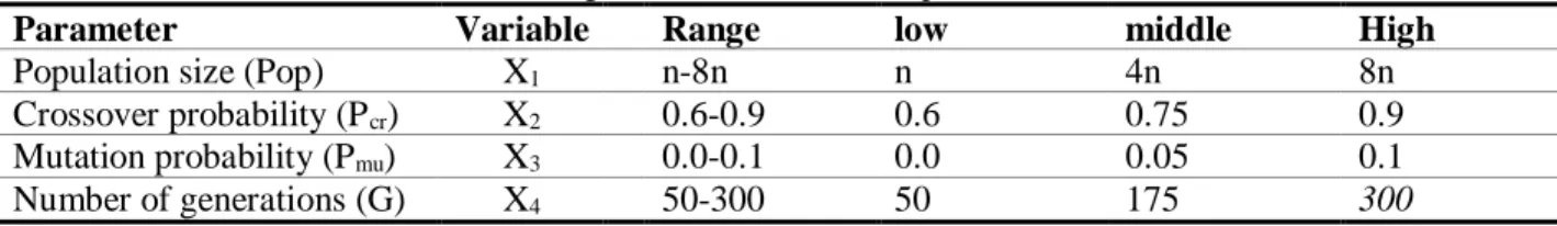
Having considered the parameters of GA as input variables and its results as output, the response surface methodology abbreviated to RSM (Myers and Montgomery, 1995) is applied for calibration. Here, the population size, crossover probability, mutation probability, and the number of generations are considered as input variables of RSM. In addition, the fitness function as accuracy index and the CPU time consumed as the time index of the algorithm are considered as outputs. To experiment RSM, we define a lower, a high, and a middle point for each variable or parameter according to table 1. In this table, n shows the number of project activities. In the RSM application, the value of parameters Pop, Pcr,
Pmu, and G are coded to -1, 0, and 1 for their low, middle, and high levels, respectively. Table 1.Search range and the levels of the input variables for the GA
High middle
low Range
Variable Parameter
8n 4n
n n-8n
X1
Population size (Pop)
0.9 0.75
0.6 0.6-0.9
X2
Crossover probability (Pcr)
0.1 0.05
0.0 0.0-0.1
X3
Mutation probability (Pmu)
300 175
50 50-300
X4
Number of generations (G)
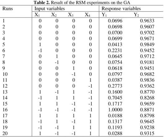
The RSM is an optimization technique to find the optimum level of a known response function obtained from a set of variables. Since such function is unknown, it makes sense to use a design that provides equal precision of estimation of the response function. The central composite face-centered (CCF) is an efficient design used for fitting a second order response function. In this research, a 24-1 fractional factorial CCF
design with 4 central points and 8 axial points, (±1,0,0,0), (0,±1,0,0), (0,0,±1,0) and (0,0,0,±1), is selected to estimate the second order function. The CCF design is shown in table 2.
Then, a set of 45 test problems generated by PROGEN including problems with 20, 30 and 40 activities and 3, 4 and 5 resources are taken into account for experiments. The test problems are solved based on different levels of CCF defined in Table 2. The first response (Y1) is the accuracy performance index of GA defined as the ratio of the solution of GA to the maximum solution detected among 20 levels. The data in column Y1 is the mean of accuracy index for 45 test problems. The higher the value of Y1 is the better performance of the GA will occur. The second response (Y2) is the CPU time performance of GA defined as the ratio of the minimum time obtained among 20 levels to the time consumed by GA for each level. The data in column Y2 is the mean of time index for 45 test problems. The higher the value of Y2 is the better the performance of GA will occur.
Table 2. Result of the RSM experiments on the GA
Runs Input variables Response variables
X1 X2 X3 X4 Y1 Y2
1 0 0 0 0 0.0696 0.9633
2 0 0 0 0 0.0698 0.9607
3 0 0 0 0 0.0700 0.9702
4 0 0 0 0 0.0699 0.9671
5 1 0 0 0 0.0413 0.9849
6 -1 0 0 0 0.2231 0.9452
7 0 1 0 0 0.0645 0.9712
8 0 -1 0 0 0.0754 0.9181
9 0 0 1 0 0.0618 0.9451
10 0 0 -1 0 0.0797 0.9682
11 0 0 0 1 0.0387 0.9836
12 0 0 0 -1 0.2773 0.9362
13 1 -1 1 -1 0.1600 0.8770
14 -1 1 1 -1 0.7045 0.8268
15 1 1 -1 -1 0.1717 0.9659
16 -1 -1 -1 -1 1.0000 0.8871
17 1 1 1 1 0.0188 0.8798
18 -1 1 -1 1 0.1317 0.9645
19 -1 -1 1 1 0.1193 0.9238
20 1 -1 -1 1 0.0288 0.9315
The results obtained from the analysis of variance of CCF are then used to estimate the second order functions for each response. The fitted responses are shown in equations (28) and (29).
2 2
1 2 3 4 1 2
2 2
3 4 2 3 2 4 3 4
1 0.969 0.019 0.026 0.007 0.009 0.012 0.015
0.027 0.007 0.026 0.005 0.007
Y X X X X X X
X X X X X X X X
(28)
2 2
1 2 3 4 1 2
2 2
3 4 2 3 2 4 3 4
2 0.058 0.198 0.035 0.029 0.176 0.108 0.021
0.020 0.082 0.146 0.036 0.036
Y X X X X X X
X X X X X X X X
(29)
The final goal of RSM is to find a desired level of the GA parameter values such that both the accuracy index and the CPU time index of the GA are simultaneously optimized. In fact, we tackle a bi-objective decision-making problem with conflicting objectives. We use the weighted additive fuzzy goal programming (Tiwari et al., 1987) which converts the model into a single objective function defined as the weighted sum of achievement degrees of the goals with respect to their target values. The method uses a single utility function to show the overall preference index, which may be any aggregated function of all achieved values of goals for each feasible solution. To solve this problem, we first need to obtain the payoff table of the positive ideal solution (PIS) as presented in table 3.
Table 3. Payoff table of PIS (in GA)
Y1 Y2
Max Y1 1.009336 0.875
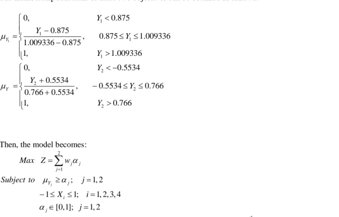
The membership functions of these two objectives can be obtained as follows:
1
1 1
1 1
0, 0.875
0.875
, 0.875 1.009336 1.009336 0.875
1, 1.009336
Y
Y Y
Y Y
(30)
2 2
2 2
0, 0.5534
0.5534
, 0.5534 0.766
0.766 0.5534
1, 0.766
Y
Y Y
Y Y
(31)
Then, the model becomes:
(32)
2 1
; 1, 2 1 1; 1, 2, 3, 4
[0,1]; 1, 2
j
j j
j
Y j
i j
Max Z w
Subject to j
X i
j
Where j and wj denote the achievement degree and the weight of the jth goal, respectively. Since the
accuracy index is more important than the CPU time index, we chose
w
1
0
.
75
andw
2
0
.
25
. Finally,the optimum values of the GA parameters are obtained and presented in Table 4.
Table 4. Optimum value of input variables for the GA
Parameter Optimum value
Population size (Pop) 8n
Crossover probability (Pcr) 0.6
Mutation probability (Pmu) 0.08
Number of generations (G) 300
3-3-Simulated annealing algorithm
The simulated annealing as a well-known local search metaheuristic starts its search on an initial solution and moves gradually toward the better solutions using a neighborhood search. Naturally, SA starts in an initial temperature (T0) and finds a number of neighborhoods in that temperature. When a
neighbor is produced, if its objective value is better than that of the current solution, it will take the position of the current solution. Even the worse neighbors have a chance to be kept alive during the search with a small probability, of course. Then, the temperature is reduced with a function named cooling scheme and again a number of neighbors are visited. As regards the problem under consideration, at first, a population of solutions is generated using two approaches previously explained in sections 3.1.1 and 3.1.2 and the best solution of the population is chosen as the initial solution of the algorithm. Then, neighbors are generated as follows:
3-3-1- Creating neighborhood and replacing
1) Generate an integer value g, uniformly distributed on the interval [1, n]. 2) According to the value of g, decide as follows:
If g n, then replace elements n and
n
1
Otherwise, generate a random value r, uniformly distributed on the interval [0, 1]. If
r
0
.
5
, replace elements g and g1, otherwise replace elements g and g1.3) Test the feasibility of the solution. If the solution is feasible, go to step 4, otherwise restore the changes and go to step 1.
4) Calculate the objective value of the neighbor called
FF
n, Let
FF
n
FF
c whereFF
crepresents the objective value of the current solution.5) Generate a random variable q, uniformly distributed between zero and one, if
0
or qe(T),replace the current solution by the neighbor, otherwise reject the neighbor and hold the current solution. (T represents the temperature at each stage)
In each temperature, a specific number of neighbors are produced and then the temperature reduces with cooling function below. Note that
T
idenotes the ith temperature and1
0
is a constant named cooling rate which is highly influential of the quality of SA’s results.1
ii
T
T
(33) The algorithm stops when the temperature reaches to a previously defined final temperature.3-3-2-Parameter calibration of SA
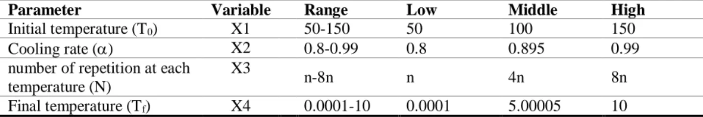
Similar to the GA, the RSM is applied to tune the SA parameters. Four parameters; initial temperature, cooling rate, number of repetition at each temperature, and final temperature are considered as input variables. Table 5 presents the search range and the levels of the input variables. In the table, n shows the number of activities of project.
Table 5. Search range and the levels of the input variables for the SA algorithm
High Middle
Low Range
Variable Parameter
150 100
50 50-150
X1 Initial temperature (T0)
0.99 0.895
0.8 0.8-0.99
X2 Cooling rate ()
8n 4n
n n-8n
X3 number of repetition at each
temperature (N)
10 5.00005
0.0001 0.0001-10
X4 Final temperature (Tf)
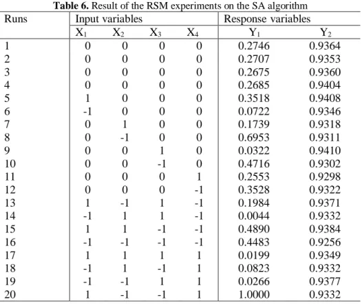
Similarly, a 24-1 fractional factorial CCF design with four central points and 8 axial points are used to
do the analysis of variance and estimate the second order response functions. Y1 and Y2 are the accuracy
index and CPU time index, respectively. Table 6 represents the input variable levels and their corresponding responses tested on 45 previously introduced problems in section 3.2.3.
Table 6. Result of the RSM experiments on the SA algorithm
Runs Input variables Response variables
X1 X2 X3 X4 Y1 Y2
1 0 0 0 0 0.2746 0.9364
2 0 0 0 0 0.2707 0.9353
3 0 0 0 0 0.2675 0.9360
4 0 0 0 0 0.2685 0.9404
5 1 0 0 0 0.3518 0.9408
6 -1 0 0 0 0.0722 0.9346
7 0 1 0 0 0.1739 0.9318
8 0 -1 0 0 0.6953 0.9311
9 0 0 1 0 0.0322 0.9410
10 0 0 -1 0 0.4716 0.9302
11 0 0 0 1 0.2553 0.9298
12 0 0 0 -1 0.3528 0.9322
13 1 -1 1 -1 0.1984 0.9371
14 -1 1 1 -1 0.0044 0.9332
15 1 1 -1 -1 0.4890 0.9384
16 -1 -1 -1 -1 0.4483 0.9256
17 1 1 1 1 0.0199 0.9349
18 -1 1 -1 1 0.0823 0.9332
19 -1 -1 1 1 0.0266 0.9377
20 1 -1 -1 1 1.0000 0.9332
Using the fuzzy goal programming for solving the functions estimated by the CCF above, the optimal values of the parameters are defined in table 7.
Table 7. Optimum value of input variables for the SA algorithm
Parameter Optimum value
Initial temperature (T0) 99.53558505 ≈ 100
Cooling rate () 0.99
number of repetition at each temperature (N) 3.2440612n ≈ 3n
Final temperature (Tf) 0.0001
4-Computational experiments
In this section, the results obtained from examining the proposed GA and SA on some test problems are reported. Collections of problems generated by PROGEN with 20, 30, 40, 80, 100, and 120 activities are considered. For the set of 20, 30, and 40 activities, a collection of 3, 4, and 5 resources, each including 10 problems is examined. For the set of 80, 100, and 120 activities, a collection of 5 test problems with 4 resources are examined. Both algorithms, GA and SA, were programmed in Matlab software and then tested on the 105 produced test problems. Moreover, the mathematical formulations of these problems are also programmed in LINGO software to compare its results with the proposed algorithms. Throughout the running of LINGO, the CPU time is limited to 1800 seconds, i.e. if LINGO could not solve a problem at this time, the process is terminated. The experiments were performed on a PC with a Pentium 2000 core2 Duo processor and 3000MB RAM. Table 8 shows the comparison results of these two algorithms and also the results of solutions found by LINGO. In this table, seven comparison criteria are utilized. The symbols of the table are defined as follows:
# : the number of instances for which the algorithm is able to found a solution before 1800 seconds #b : the number of instances for which the algorithm found a solution equal to the best solution among three ones
AAD : the average absolute deviation from the best solution known MAD : the maximal absolute deviation from the best solution known ARD% : the average relative deviation from the best solution known MRD% : the maximal relative deviation from the best solution known CPU : the average computational time of the algorithm.
Table 8. Results of the experiments for the problem
CPU time (s) MRD% ARD% MAD AAD #b # No. of problem s No. of resource s No. of
activities LING GA SA
O SA GA SA GA SA GA SA GA SA GA LING O SA GA LING O 26 14 15 31 14 18 8 100 42 53 25 0 0 10 10 10 10 10 3
20 4 10 10 10 10 10 0 0 22 55 43 89 9 19 22 32 32 15 32
32 16 13 22 8 14 5 75 32 56 22 0 0 10 10 10 10 10 5 54 36 603 64 47 42 21 167 92 110 51 0 1 9 10 10 9 10 3
30 4 10 8 10 10 8 2 0 32 130 94 196 8 33 19 54 292 34 57
59 40 256 43 13 24 8 196 63 137 39 0 1 9 10 10 9 10 5 83 73 842 50 18 32 7 239 90 161 31 0 5 5 10 10 5 10 3
40 4 10 2 10 10 2 8 0 7 121 76 185 1 20 16 32 310 72 104
103 84 450 27 3 18 0.4 174 22 122 2 0 9 1 10 10 1 10 5 421 233 - 134 0 52 0 2003 0 966 0 0 5 0 5 5 0 5 4 80 570 1017 - 35 0 28 0 1019 0 770 0 0 5 0 5 5 0 5 4 100 980 1520 - 42 0 33 0 2124 0 145 0 0 0 5 0 5 5 0 5 4 120
5-Discussion and findings
In this section the reported results are analyzed and the findings are discussed in terms of seven criteria as follows.
#-based results: according to table 8, LINGO is not able to find a solution within 1800 seconds for 4 out of 30 problems with 30 activities, 22 out of 30 problems with 40 activities, and all of 80, 100, and 120 activities while the other algorithms, GA and SA, are able to find solutions for all problems in reasonable time. These results show that the proposed metaheuristic algorithms are promising in tackling the RIP with progress payment problems since in real world large scale problems where no exact solution is available, having access to near optimal solutions is favored.
#b-based results: according to table 8, LINGO has expectedly found the best solution among other algorithms where a solution exists. In other cases, i.e. where LINGO has no solution for the problem, the GA has reached the best ones. These results demonstrate that the performance of GA is more reliable than SA since the results of GA outperform those of SA in all of 105 problems.
AAD-based results: according to table 8, the average of ADD for GA and SA in 20-activity problems is 23 and 54, respectively, in 30-activity problems are 41 and 126, respectively, and in 40-activity problems are 13 and 135, respectively which substantiates previous results displaying better performance of GA. The AAD of 13 in the last set of activities for GA is a little strange, because when the size of the problems increases, it is expected that the accuracy of a metaheuristic based algorithm like GA decreases. The only reason for such outcome is the limited access to near optimal solutions in this set of problems as LINGO has found such solution for 8 out of 30 problems. In terms of large scale problems with 80, 100, and 120 activities, as there are no solutions by LINGO and the GA has found better results in all of test problems, the ADDs of GA are zero.
MAD-based results: according to table 8, these results also support higher acceptance of GA’s results. The maximum absolute deviation for GA among all 105 problems is 94 while that is 2124 for SA. In addition, the average of MAD for GA and SA are 46 and 547, respectively denoting better efficiency of GA.
ARD%-based results: according to table 8, as expected, GA shows better results in this issue where the average of ARD% for SA (28) is more that four times of that for GA (6).
MRD%-based results: according to table 8, the MRD% for GA is smaller than that of SA in all sets of the problems confirming the better performance of GA.
CPU time-based results: according to table 8, the average of CPU time used by three methods in all 105 problems is 313, 263, and 210 seconds for LINGO, GA, and SA, respectively. This comparison demonstrates that, the more complex the problems, the more CPU time used by algorithms, nevertheless LINGO could not tackle the large scale problems in reasonable time and its CUP time used grows exponentially while proposed algorithms do not show such behavior. In addition, the CPU time used by GA is lesser than that of SA in smaller problems (30 to 80 activities) while in larger problems (100 and 120 activities) the SA consumes shorter time to reach solutions.
In a nutshell, although LINGO finds optimal solutions in small problems, it is not applicable in coping with large problems while the proposed algorithms can solve the large problems in reasonable time. In addition, GA outperforms SA in regards to the accuracy of solutions in all of test problems. Although the GA solves smaller problems in shorter time, the SA finds a solution for larger problems sooner.
6-Conclusions and recommendations for future research
In this research, a class of project scheduling problems, called resource investment problem was con-sidered. While, the RIP had been previously investigated under maximization of NPV where its payments occur at some events of the project, here the progress payment model was chosen to be combined with RIP. The mathematical formulation of the model was defined and due to NP-hardness of the problem, metaheuristic algorithms were taken into account to solve the model. Two well-known metaheuristics, SA and GA, were designed. In order to improve the efficiency of the proposed GA and SA, their parameters were statistically tuned using response surface methodology. Then, the tuned algorithms were examined on 105 test problems of small, medium, and large scales. The results of the applications of the proposed methodologies on these problems and the comparison of the results with solutions obtained from solving the mathematical formulation of the problems by LINGO software showed that the performance of GA not only is reliable when compared to LINGO results, is also highly better than SA algorithm.
Some of potential extensions of the model are considering precedence relations with minimal and maximal time lag, multi-mode execution of activities, and permitting the earliness or tardiness deviation from the due date of the project with a bonus and penalty policy.
References
Afshar-Nadjafi, B. (2014). Multi-mode resource availability cost problem with recruitment and release dates for resources. Applied Mathematical Modelling, 38(21-22), 5347-5355.
Ahuja, H. N. (1976). Construction performance control by networks. New York; Toronto: Wiley.
Demeulemeester, E. (1995). Minimizing resource availability costs in time-limited project networks. Management Science, 41(10), 1590-1598.
Doersch, R. H., & Patterson, J. H. (1977). Scheduling a project to maximize its present value: A zero-one programming approach. Management Science, 23(8), 882-889.
Drexl, A., & Kimms, A. (2001). Optimization guided lower and upper bounds for the resource investment problem. Journal of the Operational Research Society, 52(3), 340-351.
Elmaghraby, S. E., & Herroelen, W. S. (1990). The scheduling of activities to maximize the net present value of projects. European Journal of Operational Research, 49(1), 35-49.
Etgar, R. (1999). Scheduling project activities to maximize the net present value the case of linear time-dependent cash flows. International Journal of Production Research, 37(2), 329-339.
Etgar, R., Shtub, A., & LeBlanc, L. J. (1997). Scheduling projects to maximize net present value—the case of time-dependent, contingent cash flows. European Journal of Operational Research, 96(1), 90-96. Etgar, R., & Shtub, A. (1997). A branch and bound algorithm for scheduling projects to maximize net present value: the case of time dependent, contingent cash flows. International Journal of Production Research, 35(12), 3367-3378.
Grinold, R. C. (1972). The payment scheduling problem. Naval Research Logistics Quarterly, 19(1), 123-136.
Herroelen, W. S., & Gallens, E. (1993). Computational experience with an optimal procedure for the scheduling of activities to maximize the net present value of projects. European Journal of Operational Research, 65(2), 274-277.
Javanmard, S., Afshar-Nadjafi, B., & Niaki, S. T. A. (2017). Preemptive multi-skilled resource investment project scheduling problem: Mathematical modelling and solution approaches. Computers & Chemical Engineering, 96, 55-68.
Kazaz, B., & Sepil, C. (1996). Project scheduling with discounted cash flows and progress payments. Journal of the Operational Research Society, 47(10), 1262-1272.
Möhring, R. H. (1984). Minimizing costs of resource requirements in project networks subject to a fixed completion time. Operations Research, 32(1), 89-120.
Myers, R. H., Montgomery, D. C., Vining, G. G., Borror, C. M., & Kowalski, S. M. (2004). Response surface methodology: a retrospective and literature survey. Journal of quality technology, 36(1), 53-77. Najafi, A. A., & Azimi, F. (2009). A priority rule-based heuristic for resource investment project scheduling problem with discounted cash flows and tardiness penalties. Mathematical Problems in Engineering, 2009.
Najafi, A. A., & Niaki, S. T. A. (2006). A genetic algorithm for resource investment problem with discounted cash flows. Applied Mathematics and Computation, 183(2), 1057-1070.
Najafi, A. A., Niaki, S. T. A., & Shahsavar, M. (2009). A parameter-tuned genetic algorithm for the resource investment problem with discounted cash flows and generalized precedence relations. Computers & Operations Research, 36(11), 2994-3001.
Nübel, H. (1999). A branch and bound procedure for the resource investment problem subject to temporal constraints. Inst. für Wirtschaftstheorie und Operations-Research.
Nübel, H. (2001). The resource renting problem subject to temporal constraints. OR-Spektrum, 23(3), 359-381.
Qi, J. J., Liu, Y. J., Jiang, P., & Guo, B. (2015). Schedule generation scheme for solving multi-mode resource availability cost problem by modified particle swarm optimization. Journal of Scheduling, 18(3), 285-298.
Ranjbar, M., Kianfar, F., & Shadrokh, S. (2008). Solving the resource availability cost problem in project scheduling by path relinking and genetic algorithm. Applied Mathematics and Computation, 196(2), 879-888.
Rodrigues, S. B., & Yamashita, D. S. (2010). An exact algorithm for minimizing resource availability costs in project scheduling. European Journal of Operational Research, 206(3), 562-568.
Sabzehparvar, M., SEYED, H. S., & Nouri, S. (2008). A mathematical model for the multi-mode resource investment problem.
Sepil, C., & Ortac, N. (1997). Performance of the heuristic procedures for constrained projects with progress payments. Journal of the Operational Research Society, 48(11), 1123-1130.
Shadrokh, S., & Kianfar, F. (2007). A genetic algorithm for resource investment project scheduling problem, tardiness permitted with penalty. European Journal of Operational Research, 181(1), 86-101. Shahsavar, M., Najafi, A. A., & Niaki, S. T. A. (2011). Statistical design of genetic algorithms for combinatorial optimization problems. Mathematical Problems in Engineering, 2011.
Smith‐Daniels, D. E., & Aquilano, N. J. (1987). Using a late‐start resource‐constrained project schedule to improve project net present value. Decision Sciences, 18(4), 617-630.
Tiwari, R. N., Dharmar, S., & Rao, J. R. (1987). Fuzzy goal programming—an additive model. Fuzzy sets and systems, 24(1), 27-34.
Vanhoucke, M., Demeulemeester, E., & Herroelen, W. (1999). Scheduling projects with linear time-dependent cash flows to maximize the net present value.
Yamashita, D. S., Armentano, V. A., & Laguna, M. (2006). Scatter search for project scheduling with resource availability cost. European Journal of Operational Research, 169(2), 623-637.
Zimmermann, J., & Engelhardt, H. (1998). Lower bounds and exact algorithms for resource leveling problems. Report WIOR-517, University Karlsruhe.
Zoraghi, N., Shahsavar, A., Abbasi, B., & Van Peteghem, V. (2017). Multi-mode resource-constrained project scheduling problem with material ordering under bonus–penalty policies. Top, 25(1), 49-79.