Solving a location-allocation problem by a fuzzy self-adaptive NSGA-II

18

Solving a Location-Allocation problem by a fuzzy self-adaptive

NSGA-II

Hossein Salehi

1

, Reza Tavakkoli-Moghaddam

2*

,

Ata Allah Taleizadeh

2

, Ashkan

Hafezalkotob

1

1 _{School of Industrial Engineering, South Tehran Branch, Islamic Azad University, Tehran, Iran} 2_{School of Industrial Engineering, College of Engineering, University of Tehran, Tehran, Iran}

[email protected], [email protected], [email protected], [email protected]

Abstract

This paper proposes a modified non-dominated sorting genetic algorithm (NSGA-II) for a bi-objective location-allocation model. The purpose is to define the best places and capacity of the distribution centers as well as to allocate consumers, in such a way that uncertain consumers’ demands are satisfied. The objectives of the mixed-integer nonlinear programming (MINLP) model are to (1) minimize the total cost of the network and (2) maximize the utilization of distribution centers. To solve the problem, a fuzzy modified NSGA-II with local search is proposed. To illustrate the results, computational experiments are generated and solved. The experimental results demonstrate that the performance metrics of the fuzzy modified NSGA-II is better than the original NSGA-II.

Keywords: Location-Allocation, fuzzy rule base, multi-objective evolutionary algorithm.

1- Introduction

Supply chain network design (SCND) models have been noticed by many researchers as an essential problem in determining the supply chain’s structure. Multiplicities of decisions affect the SCND. Supply chain (SC) decisions involve strategic (i.e., location of facilities and capacity of facilities), tactical (i.e., flow of products, transportation mode and inventory) and operational (i.e., fulfilment of customer demands and pricing) decision levels. A key determination connected to the design and performance of a SC is the definition of the optimal or near-optimal locations for distribution centers (DC). Some investigations have been noticed inventory management models in the SCND as a location-inventory (L-I) problems (Mousavi et al., 2015; Salehi et al., 2015; Kaya and Urek, 2016; Puga and Tancrez, 2016; Zahiri et al., 2018).

Ahmadi et al. (2016) presented a bi-objective model that maximizes the total profit and minimizes the customer dissatisfaction. They proposed a three-level SC considering L-I decisions with capacitated in-house fleet, proactive lateral-transhipments between facilities and multiple products. Mehrabad et al. (2017) developed a four-echelon SC with multi-objective model in order to optimize the total cost of the network and the finishing rate. Variables and parameters of their research are related with transportation, manufacturer’s location, distribution of the products from manufacturers

*Corresponding author

ISSN: 1735-8272, Copyright c 2020 JISE. All rights reserved

Journal of Industrial and Systems Engineering Vol. 12, No. 4, pp. 18 - 26

19

to DCs, and inventories. They proposed a multi-objective evolutionary meta-heuristic algorithm based on the particle swarm. Soolaki and Arkat (2017) considered a location-allocation problem and integrated cellular manufacturing system into a three-level SC. Yadegari et al. (2018) extended a mathematical closed-loop SCND model with the multi-period, multi-echelon and considering inventory cost. They developed a Memetic algorithm by combinatorial local search method based on the nature of the multi-part solution representation.

Zheng et al. (2019) studied a single product L-I problem by considering routing in SC. In their model demands were considered independent and uncertain which follow the normal distribution. The objective function is to minimize the total cost (such as installation cost, inventory cost, and transportation cost). They introduced real-world constraints into the integrated model and developed an exact solution method based on the Generalized Benders Decomposition to solve the mathematical model. Zhen et al. (2018) developed a mathematical closed-loop SCND under uncertainty to determine the location of DCs and their capacities and define the flow of goods in forward and reverse directions. They converted the stochastic non-linear model to a conic quadratic mixed integer programming model and solved it by CPLEX.

In general, the SCND has been considered as a single-objective problem; however, it involves more than one objective. Multi-objective evolutionary algorithms (MOEA) have been considered for solving multi-objective mathematical models. One of the first MOEA is the non-dominated sorting genetic algorithm (NSGA) developed by Srinivas and Deb (1994) finding a set of Pareto-optimal solutions. Deb, et al., (2002) extended and improved the NSGA with the concept of the crowding distance, namely NSGA-II, which ranks and selects the population fronts. Like the genetic algorithm (GA), the performance of II is affected by its parameters; therefore, a fuzzy modified NSGA-II with local search, namely FMNSGA-NSGA-II, is proposed to solve the presented model. The remainder of this paper is organized as follows. Section 2 presents the multi-objective model for the SCND problem. Section 3 proposes the FMNSGA-II. The numerical outcome and computational results are presented in section 4. Finally, section 5 presents conclusions.

2- Problem description and formulation

The considered supply chain network consists of a fixed location manufactory, distribution centres (i.e., warehouses) and retailers (i.e., customers). The demands of customers are stochastic. The proactive lateral transhipment policy with partial pooling can be used through DCs. Accordingly, in the real world; the model is intended for supply chains of industries, such as clothing, pharmaceutical and food.

2-1- Notations

The following notations are used in order to model the given problem.

Indices:

m Set of consumers



m1, ..., M



,

n h Set of candidate DCs



n h, 1, ..., N



p _{Set of products}



_{l1, ..., P}



k Set of capacity levels



k1, ..., K



Parameters: mnp

T Transportation cost from DCs to consumers

np

T Transportation cost from the manufactory to DCs

nhp

LC Transportation cost between DCs

nk

F Installation cost of DCs

mp

d Mean of the demand

mp

v Variance of the demand

np

20

np

H Keeping cost

np

R Fixed order cost

mk

cap DCs’ Capacity

p

s Space requirement of products

PH Planning horizon

Decision variables: nk

Z 1 if the nk-th DC is opened; 0, otherwise

mnp

Y 1 if the m-th consumer is assigned to the n-th DC for the p-th product; 0, otherwise

nhp

Y 1 if the j-th DC is served with the h-th DC for the p-th product; 0, otherwise

np

D Mean demand of the product number p that covered to the n-th DC from the manufactory

np

DT Mean demand of the p-th product that covered to the n-th DC from other DCs

np

V Variance of demand of the product number p covering to the n-th DC

nhp

a Percentage demands of the p-th product that covered to the n-th DC from the h-th DC

2-2- Mathematical model

Inventory is one of the significant elements of a SC. To determine the inventory cost of the network, the continuous inventory revision (𝑟, 𝑄) is considered. So, by considering the inventory system we can calculate the service level as:

 



D np np



1

Prob  L r   (1)

According to the (1), the reorder point of the product number p in the n-th DC is rnp D SSnp,

where SSnpis the safety stock of the inventory system, and the mean demand of the product number p

is D, assigned to the n-th DC. When the demand is stochastic (based on a normal distribution

function with a given probability1); SSnpcan be determined by:

1 . .

np np np

SS  Z  L V (2)

The variance of demand of the product number p covering to the n-th DC is obtained by:





2 ₂

1 1 1 1

1 . . . . . .

M N np nhp nhp mp mnp

M N

m h

hnp mp hnp mhp m h

V a Y v Y a v Y Y

   





 



(3)

According to the basic economic ordering quantity (EOQ) inventory model, the inventory system’s whole cost is calculated based on equation (4). The mean demand of the product number p that covered to the n-th DC from the manufactory

 

Dnp is calculated based on equation (5).

1 1

2 . . . .

P

np n N

D n p

p np np np

R  H H SS

 





(4)

1 1 1

. . . .

M M N

h

np mp mnp np mp hnp mhp p

m m h

n

D d Y a d Y Y DT

  









 (5)

where DTnp is the mean demand of the p-th product that covered to the n-th DC from other DCs, and calculated by:

1 1

. . .

M N

np nh

m

p mp nhp mnp h

DT a d Y Y

 





(6)

So the mean demand of the p-th product, assigned to the n-th DC is calculated by Dnp  Dnp  DTnp

21





1 1

2 . . .

N P

np np n n

p p

p n

H R D DT

 





(7)

1 1 1

. . .

N P

n p

np np np

H Z_ L V

 





By adding the costs of DC installing with a planning horizon (PH) to variable costs and considering the average utilization DCs as the second objective, the mathematical multi-objective model of the SCND problem through the lateral transhipment policy is as follows:

1

1 1 1 1 1 1 1

Min . . . . . .

N N P M N P

n

p

p _{np mnp mp mnp} K

nk nk

n k n p m n

W F Z PH T D PH T d Y

      













(8)





1 1 1 1 1 1

1 1 1

. . . . . . 2 . . .

. . . .

mp np n

M N N P N P

nhp nhp nh p np np

m n h p n p

np np np

n p

p mnp

N P

PH LC a d Y Y PH H R D DT

PH H Z  L V

            











1 2

1 1 1

1 .

Max /

. K np np p nk K

n _n n k

P

N N

p

k nk k

s D DT

W Z cap Z       









(9) s.t. 1 1 N np n m Y  



;m p, (10)

1 1 N nhp h m M mnp Y Y   





;n p, (11)

1 1 0 N P nnp n p Y   



(12)





1 1

. .

P

p np np nk n K

k

p k

s D DT cap Z

 

 





;n (13)

1 1 K nk k X  



;n (14)

 

, , 0,1

nk mnp nhp

Z Y Y  ;m n p k, , , (15)

np

DT  Z ; n (16)

Equations (10) and (11) show the single source assumption. Equation (12) ensures that there is no internal transhipment in any DCs. Equation (13) shows the capacity level constraint. Equation (14) warrants that each DC can be established on a unique capacity level. Finally, constraints (15) and (16) state the integer and real number variables, respectively.

3- Solution algorithm

The main components of the FMNSGA-II are described below.

3-1- Initialization

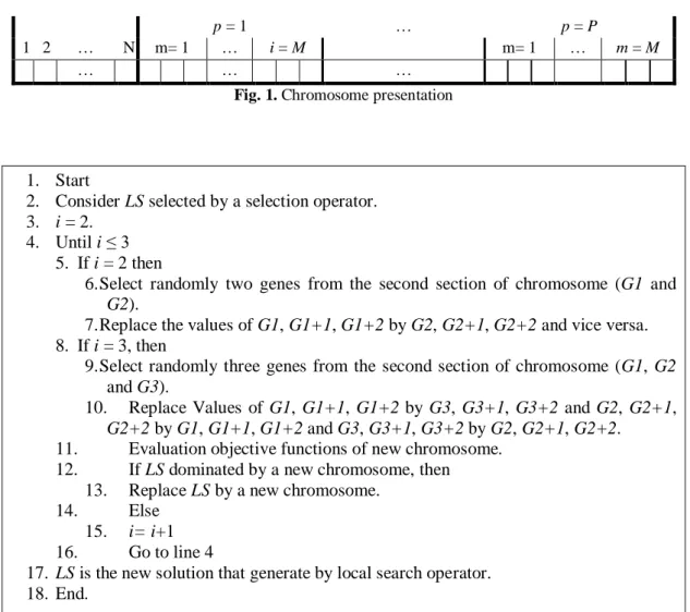
The proposed chromosome structure is shown in figure 1. Each chromosome consists of two sections. As shown in this figure, the first section consisting of J genes is related to location and capacity level decisions. Those genes can obtain content in [0, k]. The second section is related to allocation and lateral transhipment decisions and consists of L sub-sections for products, in which each sub-section consists of I part for customers whom each part has three genes. The first gene value

22

in each part (taking a value between [0, J]) is related to allocation variables. The second gene (taking a value between [0, J]) is related to lateral transhipment variables, and the third gene (taking a value between zero to1) refers a constant of ajhlvariables.

3-2- Non-dominated sorting

To prepare a diverse front, a crowding distance (CD) is calculated for each solution as given in (17). The individuals with a lower value of a CD are preferred over the individuals with a higher value of a CD in a selection procedure.

1 1

1

i i K

k k i Max Min

k k k

Z Z

CD

Z Z

 

  





(17)

The notation K in equation (17) is the number of objectives, i k

Z is the k-th objective of the i-th individual, Max

k

Z is the maximum value of the k-th objective in the front, and Min k

Z is the minimum value of the k-th objective in the front.

p = P

…

p = 1

m = M

… m= 1

i = M

… m= 1 N … 2 1

… …

…

Fig. 1. Chromosome presentation

1. Start

2. Consider LS selected by a selection operator. 3. i = 2.

4. Until i ≤ 3 5. If i = 2 then

6.Select randomly two genes from the second section of chromosome (G1 and

G2).

7.Replace the values of G1, G1+1, G1+2 by G2, G2+1, G2+2 and vice versa. 8. If i = 3, then

9.Select randomly three genes from the second section of chromosome (G1, G2

and G3).

10. Replace Values of G1, G1+1, G1+2 by G3, G3+1, G3+2 and G2, G2+1,

G2+2 by G1, G1+1, G1+2 and G3, G3+1, G3+2 by G2, G2+1, G2+2. 11. Evaluation objective functions of new chromosome.

12. If LS dominated by a new chromosome, then 13. Replace LS by a new chromosome.

14. Else 15. i= i+1 16. Go to line 4

17. LS is the new solution that generate by local search operator. 18. End.

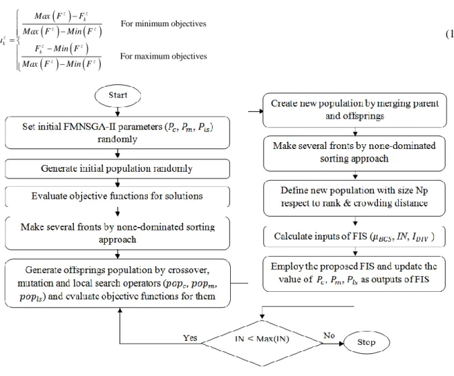
Fig. 2. Local search algorithm

3-3- Crossover, mutation and local search

The tournament selection operator is used to create the offspring population. Then, the crossover operator with respect to the crossover rate

 

P_c generates new children. After applying the crossover operator, more solutions are created by using the mutation operator with respect to the mutation rate

23

NSGA-II is the 2-opt and 3-opt local search operators as described in Fig. 2. A local search rate

 

P_ls

indicates how often this operator will be performed.

3-4- Fuzzy adaptive operators

To improve the performance and quality of the proposed algorithm, a fuzzy inference system (FIS) is used to adaptP_c, P_mandP_lsdynamically. Thus, a three-input, three-output, eight-rule FIS is developed. The Mamdani type is applied as an inference process. Three functions are proposed as the inputs of the FIS (Sardou and Ameli, 2016). The first function is the total normalized fitness value of the best comprehensive solution



_BCS



. The total normalized fitness value of the k-th solution (i.e.,_k) is computed by:

1

Z _z k z k

Z



 _



 ₍₁₈₎

where z k

 is the normalized value of the z-th objective function for the k-th solution, which is calculated by:

 

 

 

 

 

 

For minimum objectives

For maximum objectives

z z

k

z z

z

k _{z z}

k

z z

Max F F Max F Min F

F Min F Max F Min F 

 



 

   

 _



(19)

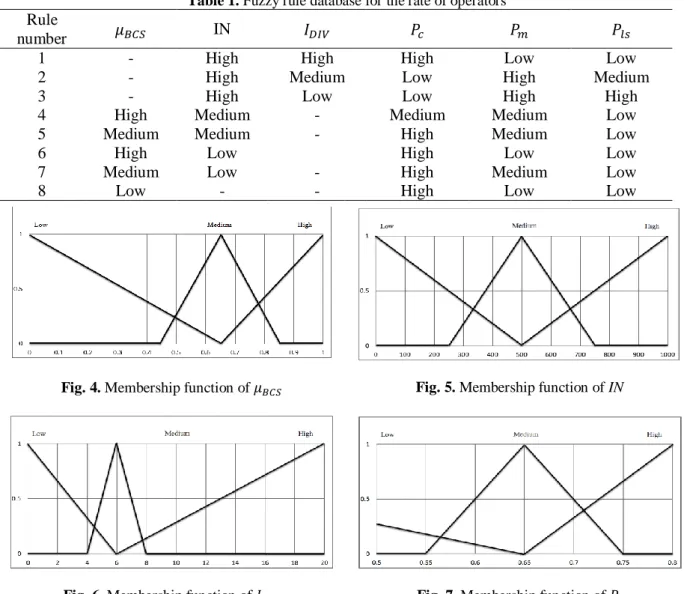
Fig. 3. Flowchart of the FMNSGA-II

where z k

F denotes the real value of the z-th objective function in the k-th efficient solution. The second function (as the input of the FIS) is the iteration number (IN), and the third function is the index of diversity (IDIV) that is equal to the summation of the CD of each solution. The value of

𝜇𝐵𝐶𝑆 is expected to improve in each iteration. Therefore, if 𝜇𝐵𝐶𝑆 does not get better impressively over

a number of iterations (IN), then for the next iteration, IN is considered to affect the value of pc, pm and

diversity along the non-dominated front. Hence, IDIV is taken into account to make changes in pc, pm

and pls. Fig.3 shows a graphical representation of the FMNSGA-II for the multi-objective SCND. The membership functions of three inputs and three outputs shown in the figures 4 to 9, respectively. The fuzzy rules are shown in Table 1. In addition, the centroid calculation is applied as a defuzzification method.

Table 1. Fuzzy rule database for the rate of operators

Rule

number 𝜇𝐵𝐶𝑆 IN 𝐼𝐷𝐼𝑉 𝑃𝑐 𝑃𝑚 𝑃𝑙𝑠

1 - High High High Low Low

2 - High Medium Low High Medium

3 - High Low Low High High

4 High Medium - Medium Medium Low 5 Medium Medium - High Medium Low

6 High Low High Low Low

7 Medium Low - High Medium Low

8 Low - - High Low Low

Fig. 4. Membership function of 𝜇𝐵𝐶𝑆 Fig. 5. Membership function of IN

Fig. 6. Membership function of 𝐼𝐷𝐼𝑉 Fig. 7. Membership function of 𝑃𝑐

Fig. 8. Membership function of 𝑃𝑚 _{Fig. 9. Membership function of} 𝑃_𝑙𝑠

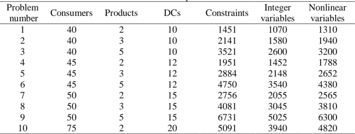
Table 2. Test problems Nonlinear variables Integer variables Constraints DCs Products Consumers Problem number 1310 1070 1451 10 2 40 1 1940 1580 2141 10 3 40 2 3200 2600 3521 10 5 40 3 1788 1452 1951 12 2 45 4 2652 2148 2884 12 3 45 5 4380 3540 4750 12 5 45 6 2565 2055 2756 15 2 50 7 3810 3045 4081 15 3 50 8 6300 5025 6731 15 5 50 9 4820 3940 5091 20 2 75 10

4- Computational results

As described at table 2 several different test problems, with various sizes developed as the computational experiments. Consumer’s value and potential DC zones are from 40 to 75 and 10 to 20, respectively. The quantities of products are from {2,3,5} and capacity levels are from {1: 5}.To obtain the performance of the proposed algorithm, the results of FMNSGA-II are compared with the original NSGA-II. The parameters of NSGA-II are defined by Taguchi technique (Sadeghi et al., 2014). Two algorithms are coded with Matlab2013, and run 10 times on a PC (i5-CPU at 2.67 GHz, 4.00 GB of RAM), in which the best run of each test problem is selected for comparison.

Table 3 shows comparison between the results. According to this table, three different performance metrics are used for the experiments (Deb, 2001) such as spacing (SP), generational distance (GD), spread (∆).It is observed that the performance of the FMNSGA-II, except the execution times, is better than the NSGA-II with respect to the mean values of metrics.

Table 3. Comparison of the performance metrics

Problem

number NSGA-II FMNSGA-II

SP GD ∆ Time SP GD ∆ Time 1 0.0136 0.0181 0.9824 577 0.0111 0.0146 0.8248 673 2 0.0078 0.0391 1.0577 719 0.0061 0.0244 0.9112 871 3 0.0024 0.0318 1.0101 987 0.0006 0.0014 1.0021 1199 4 0.0049 0.0437 1.0337 755 0.0086 0.0422 1.0058 906 5 0.0049 0.0130 0.9787 994 0.0061 0.0133 1.0390 1221 6 0.0050 0.0570 1.0254 1435 0.0031 0.0085 1.0191 1778 7 0.0113 0.0204 0.9670 1088 0.0058 0.0110 1.0145 1321 8 0.0027 0.0057 1.0145 1462 0.0027 0.0181 1.0147 1759 9 0.0078 0.0250 0.6852 2218 0.0050 0.0056 0.8436 2866 10 0.0076 0.0225 1.0126 2356 0.0119 0.0202 0.7503 2937 Ave. 0.0068 0.0276 0.9767 1259 0.0061 0.0159 0.9425 1553

5- Conclusions

A multi-objective SCND problem was considered to determine the location of DC sites and flows of goods through the chain. In addition, the proactive lateral transhipment policy with partial pooling was considered. It is found that the performance of the NSGA-II is dependent on its parameters. So a fuzzy inference system can be used to create a more efficient algorithm. Therefore, FMNSGA-II proposed to solve the MINLP model. The FMNSGA-II parameters were self-adaptive via the fuzzy inference system. To determine the efficiency of the proposed algorithm, 10 different problems with various sizes were generated randomly. These test problems are solved by the FMNSGA-II and standard

NSGA-II, in which the results showed that the performance metrics which obtained by the FMNSGA-II are better than NSGA-FMNSGA-II. It can be concluded that by improving the quality of the results in this method, in comparison with the previous method, the decision variables are determined, which will increase the utilization of the DCs and reduce the total cost of the chain. Reactive lateral transshipment policy can be considered as an extension of this paper for future research.

References

Ahmadi, G., Torabi, S.A., and Tavakkoli-Moghaddam, R. (2016). A bi-objective location-inventory model with capacitated transportation and lateral transshipments, Int. J. of Production Research, 54(7), 2035-2056.

Deb, K. (2001). Multi-objective optimization using evolutionary algorithms. John Wiley & Sons.

Deb, K., Pratap, A., Agarwal, S. and Meyarivan, T. (2002). A fast and elitist multiobjective genetic algorithm: NSGA-II. IEEE Transactions on Evolutionary Computation, 6(2), 182-197.

Kaya, O. and Urek, B. (2016). A mixed integer nonlinear programming model and heuristic solutions for location, inventory and pricing decisions in a closed loop supply chain. Computers & Operations Research, 65, 93-103.

Mehrabad, M.S., Aazami, A. and Goli, A. (2017). A location-allocation model in the multi-level supply chain with multi-objective evolutionary approach. Journal of Industrial and Systems Engineering, 10(3), 140-160.

Mousavi, S., Alikar, N., Niaki, S. and Bahreininejad, A. (2015). Optimizing a location allocation-inventory problem in a two-echelon supply chain network: A modified fruit fly optimization algorithm. Computers & Ind. Eng., 87, 543-560.

Puga, M. and Tancrez, J. (2016). A heuristic algorithm for solving large location–inventory problems with demand uncertainty. European Journal of Operational Research, 259(2), 413-423.

Sadeghi, J., Sadeghi, S. and Niaki, S.T.A. (2014). A hybrid vendor managed inventory and redundancy allocation optimization problem in supply chain management: An NSGA-II with tuned parameters. Computers & Operations Research, 41, 53-64.

Salehi, H., Tavakkoli-Moghaddam, R. and Nasiri, G. (2015). A multi-objective location-allocation problem with lateral transshipment between distribution centres. International J. of Logistics Systems and Management, 22(4), 464-482.

Sardou, I. and Ameli, M. (2016). A fuzzy-based non-dominated sorting genetic algorithm-II for joint energy and reserves market clearing. Soft Computing, 20(3), 1161-1177.

Soolaki, M. and Arkat, J. (2018). Supply chain design considering cellular structure and alternative processing routings. Journal of Industrial and Systems Engineering, 11(1), 97-112.

Srinivas, N. and Deb, K. (1994). Muiltiobjective optimization using nondominated sorting in genetic algorithms. Evolutionary Computation, 2(3), pp. 221-248.

Yadegari, E., Alem-Tabriz, A. and Zandieh, M. (2019). A Memetic Algorithm with a Novel Neighborhood Search and Modified Solution Representation for Closed-loop Supply Chain Network Design. Computers & Industrial Engineering, 128, 418-436.

Zahiri, B., Jula, P. and Tavakkoli-Moghaddam, R. (2018). Design of a pharmaceutical supply chain network under uncertainty considering perishability and substitutability of products. Information Sciences, 423, 257-283.

Zhen, L., Wu, Y., Wang, S., Hu, Y. and Yi, W. (2018). Capacitated closed-loop supply chain network design under uncertainty. Advanced Engineering Informatics, 38, 306-315.

Zheng, X., Yin, M. and Zhang. Y. (2019). Integrated optimization of location, inventory and routing in supply chain network design. Transportation Research Part B, 121, 1-20.