Learning from Time Series: Supervised Aggregative Feature Extraction
Andrea Schirru, Gian Antonio Susto, Simone Pampuri and Se´an McLoone
Abstract— Many modeling problems require to estimate a scalar output from one or more time series. Such problems are usually tackled by extracting a fixed number of features from the time series (like their statistical moments), with a consequent loss in information that leads to suboptimal pre-dictive models. Moreover, feature extraction techniques usually make assumptions that are not met by real world settings (e.g. uniformly sampled time series of constant length), and fail to deliver a thorough methodology to deal with noisy data. In this paper a methodology based on functional learning is proposed to overcome the aforementioned problems; the proposed Supervised Aggregative Feature Extraction (SAFE) approach allows to derive continuous, smooth estimates of time series data (yielding aggregate local information), while simultaneously estimating a continuous shape function yield-ing optimal predictions. The SAFE paradigm enjoys several properties like closed form solution, incorporation of first and second order derivative information into the regressor matrix, interpretability of the generated functional predictor and the possibility to exploit Reproducing Kernel Hilbert Spaces setting to yield nonlinear predictive models. Simulation studies are provided to highlight the strengths of the new methodology w.r.t. standard unsupervised feature selection approaches.
INTRODUCTION
Machine learning methodologies are nowadays applied in many industrial and scientific environments including technology-intensive manufacturing [5], biomedical sciences [6], and in general every data-intensive field that might ben-efit from reliable predictive capabilities. Machine learning techniques exploit organized data to create mathematical representations (models) of an observable phenomenon. It is then possible to rely on such a model to provide predictions for unobserved data. In mathematical terms, let
S=xi∈R1×p, yi∈R Ni=1 (1)
be a training dataset of N observations of a certain phe-nomenon. The i-th observation is characterized by pinput features, constituting the vectorxi, and a scalar target value
yi. In practical terms, the input space usually relates to easily obtained data, while the target value is either not always available or results from a costly procedure; in a typical industrial application,xi would collect sensor readings dur-ing a process operation, while yi would be a quantitative indicator of product quality. The goal is then to exploit the
A. Schirru and S. Pampuri are with University of Pavia, Italy. E-mail: {andrea.schirru, simone.pampuri}@unipv.it
G.A. Susto is with University of Padova, Italy. E-mail:
S. McLoone is with National University of Ireland, Maynooth, Ireland. E-mail:[email protected]
The financial support of the Irish Centre for Manufacturing Research and Enterprise Ireland (grant CC/2010/1001) are gratefully acknowledged.
information provided by S to create a predictive model f
such that, given a new observationx /˜∈ S,f(˜x)will provide an accurate prediction of the unobserved y˜: in the case of the above mentioned industrial example, the modelf would be able to estimate the final product quality relying only on sensor readings collected during process operation. It is important to note that in real life applications data is rarely (if ever) organized in a convenientN×pmatrix ready to serve as input for a machine learning procedure. Indeed, the transition from a real life object to its mathematical representation will necessarily destroy part of the original information.
In this paper, we consider the learning problem where the input information is conveyed in the form of time series; more specifically, every observation of the phenomenon is described by ptime series, that we know through an array of irregularly sampled measurements whose size can vary observation-wise. This setting relates to a common problem in predicting process results in an industrial setting [8], where the input space is often represented by non-uniformly sampled sensor readings. The challenge is to aggregate the information contained in each time series so that summary features are produced that are good predictors of the tar-get value. Assuming the existence of a continuous process underlying such sensor readings, we adopt a functional learning paradigm in order to tackle the presented problem: specifically, we discuss suitable estimation techniques to reconstruct the original continuous time series and derive a feature extraction technique that can be employed with regular machine learning techniques, which we refer to as Supervised Aggregative Feature Extraction (SAFE). Further-more, we prove the advantage of the proposed methodology w.r.t. other approaches by means of numerical simulations. The remainder of the paper is organized as follows: Section I provides a mathematical formalization of the problem at hand, as well as an overview of some feature extraction techniques for time series. Section II presents and discusses the proposed SAFE methodology for time series feature extraction, while Section III is devoted to underpinning basis expansion strategies and nonlinear regression techniques. Finally, Section IV validates the proposed methodology by means of numerical simulations. After the final remarks, Appendix A is devoted to mathematical proofs.
I. PROBLEM STATEMENT
GivenN observations consisting ofp time series, where thei-th observation Xi is defined as
Xi= [x (1) i (t) . . . x (j) i (t) . . . x (p) i (t)], t∈[0,1],∀ j
51st IEEE Conference on Decision and Control December 10-13, 2012. Maui, Hawaii, USA
and a scalar target variableyi, let the training set be S={Xi, yi}
N i=1
The goal is then to learn, relying onS, a predictor function
f. Such a predictor must be optimal in the sense that, given a new inputXnew,f(S,Xnew)will be close (in the sense of a normed distance) to the unobservedynew.
In practice, the continuous time series x(ij)(t) are not available: instead it is necessary to rely on a set of discrete samplesnt(i,sj), z (j) i,s oNi,j s=1 wheret (j) i,s andz (j)
i,s are the time and value of thes-th sampled point from thej-th time series of thei-th observation. In general, the series may have difform length (such that Ni,j6=Ni,m, Ni,j 6=Nk,j) and sampling timestamps (t(i,sj)6=t (m) i,s , t (j) i,s 6=t (j)
k,s). Furthermore, the noise of the channel needs to be taken into account:
zi,s(j) = x (j) i (t (j) i,s) +v (j) i,s vi,s(j) ∼ N(0, ρ 2 j)
In order to employ machine learning techniques to find f, two main issues must be addressed: (i) it is in general necessary to extract a homogeneous set of features from every observation, and (ii) it is not possible to know in advance what part of the time series (if any) has an impact on the target variable. This lack of information must be taken in account when choosing a feature extraction methodology: indeed, a representation based solely on the global features of a dataset is likely to yield suboptimal predictions. In the next subsection, some of the most common feature extraction techniques for time series are presented and discussed.
A. Feature extraction
The extraction of a set of features from an observation will result in the loss of some information, especially when the format of such information is expected to show inter-example differences, such as in the presented case where difform sampling times and length are present. The goal is to build a regressor matrix Φ ∈ Rn×p, whose entry (i, j)
represents thej-th feature of thei-th observation that can be subsequently used, along with the target variable vectorY ∈ Rn, to train a predictor using a machine learning algorithm.
One of the simplest approaches is to rely on statistical moments: givenptime series, let us buildΦas
Φ = [Φ1 . . . Φj . . .Φp] where the[i, k] element ofΦj∈Rn×kmax is
Φj[i, k] =m(k) n
zi,s(j)oNi,j
s=1
Here kmax is the highest considered moment order and
m(k)(·)is thek-th sample moment of the input time series.
It is immediately evident that this approach suffers from a major drawback, namely the inability to consider the depen-dency between information and time. Furthermore, it should be noted that the sample estimators of statistical moments are consistent forindependentdata points: it follows that, in
the quite common case of autocorrelated time series, such estimates bear very little statistical meaning.
A more sophisticated approach consists of a systematic sampling of the input time series: specifically, the interval [0,1]is divided intoN segments[τ1 . . . τN]. The regressor matrix is then populated with the segment-wise averages, as
Φj[i, k] = Avg[z
(j)
i,s :t
(j)
i,s ∈τk].
When using this approach it is necessary to select the number of segments, N, in advance: this usually translates to a trade-off decision between locality (temporal resolution) and stability of information (robustness to noise). Furthermore, in the case of difform sampling, different features are likely to be computed from a different number of values, as the distribution of sampling points would privilege some segments over the others: this can potentially lead to data reliability issues. In order to overcome such instabilities, it is possible to project the rows of theΦmatrix obtained using the sampling approach on their direction of main variance. This yields the Principal Component Analysis (PCA) [4] transformation of the sampled input space.
B. Elements of machine learning and regularization
Once Φ is obtained, it is possible to employ a machine learning technique to find a predictor model f. As a first assumption, let the structure of the model be specified by a vector of parametersθ. Consider the fitness function
L(θ) =F(θ) +λR(θ) (2) and the solution of the optimization problem
θ∗= arg min θ L(θ).
The error term F measures the approximation power of
f (w.r.t. S), while the regularization term R measures the complexity of the model. Furthermore,λ≥0 is a hyperpa-rameterthat acts as a tuning knob for the trade-off between approximation and variability: too small a value results in an overfitted model (specifically tuned on the training set, with low predictive power), while too large a value results in an underfitted model (which would not incorporate the necessary information for making good predictions). The insight is that the correct value of λ would result in only the relevant information being incorporated into the model, yielding the highest predictive power.
While a wide variety of choices are possible for both F
and R, most learning techniques require the minimization problem to be convex w.r.t.θ; to exploit this desirable feature, it is sufficient for F and R to be convex. Notably, if f is defined as a linear function ofθsuch as
f(Φ;θ) := Φθ
andF is the sum of squared estimation residuals
F:=||Y −f(Φ;θ)||2=||Y −Φθ||2
the global minimum of F can be expressed in closed form as theleast squares solution
Equation (3) is prone to numerical issues and instability, since there is no guarantee that Φ0Φ will be full rank or well conditioned. A modification that preserves this closed-form solution and resolves instability issues is represented by Ridge Regression (RR), obtained by setting
R(θ) :=θ0θ=X i
θ2i. The global RR minimizer is then
θ∗= (Φ0Φ +λI)−1Φ0Y (4)
In order to obtain a nonlinear modelf without giving up the desirable convexity features of the optimization problem, it is possible to exploit thekernel trick [1] to embed a nonlinear projection of Φ on a Reproducing Kernel Hilbert Space (RKHS) [2] in a quadratic optimization problem. Noting that
(Φ0Φ +λI)−1Φ0 = Φ0(ΦΦ0+λI)−1 equation (4) may be rewritten as
θ∗= Φ0(ΦΦ0+λI)−1Y
and the predictionf(Φnew)as
f(Φnew) =hΦnew,Φi(hΦ,Φi+λI)−1Y (5) By replacing the linear inner product h·,·i with a nonlinear positive definite kernel functionK, theKernel Ridge Regres-sion[10] coefficient vector ccan be defined as
c∗= (K(Φ,Φ) +λI)−1Y
and the corresponding predictorf is given by
f(Φnew) =K(Φnew,Φ)c∗
Thus, the resulting model yields nonlinear predictions w.r.t. the elements of the regressor matrix. A thorough review of machine learning techniques and Kernel-based techniques is beyond the scope of this paper. The interested reader is referred to [4] and [9].
II. SUPERVISED AGGREGATIVE FEATURE EXTRACTION
In this section the proposed supervised aggregative feature extraction (SAFE) methodology is presented and motivated from a theoretical point of view. In order to introduce SAFE, we consider an ideal case, in which the continuous functions
x(ij)(t) are known and available. Employing the functional regression paradigm, consider the following definition off:
f(Xi) := p X j=1 D x(ij)(t), β (j)(t)E L2 (6)
where hf, giL2 is the L2 inner product of real functions f andg, defined as
hf, giL2 = Z ∞
−∞
f(t)g(t)dt
It is apparent how the predictor defined by (6) assumes that the continuous phenomenonxinfluences the target variable
y through a weighted integration with an unknown shape
functionβ. In the following we focus on the sum of squared residuals approximation error term, defined as
F(β) = N X i=1 p X j=1 Z ∞ −∞ β(j)(t)x(j) i (t)dt−yi 2 (7) It is then possible to introduce the functional learning opti-mization problem:
β∗ = arg min
β F(β) +λR(β) (8)
β = hβ(1)(t), β(j)(t), β(p)(t)i (9)
whereF(β)is defined in (7) and R(β) is a regularization term that penalizes the variability ofβ: for example,
R(β) = p X j=1 D β(j), β(j)E L2
It is apparent that the shape functionsβ(·)(t)are functional
parameters of the optimization problem (9). It is to be noted that it is not possible to directly handle (7) for two reasons: (i) the functions x(ij)(t) are observed only through a finite number of noisy, irregularly sampled data points; (ii) the generic functionsβ(j)(t)have infinite degrees of freedom. To
overcome such issues and solve (9), the next sections present a Gaussian process estimation of the unobserved time series and propose a parametrization for the shape functionsβ.
A. Time series approximation
Consider an approximation of the fitness functionL
ˆ
L= ˆF+λR
where the approximated loss function is defined as ˆ F= N X i=1 p X j=1 Z ∞ −∞ β(j)(t)ˆx(j) i (t)dt−yi 2
andxˆ(ij)(t)is an estimate of the unobservedx
(j)
i (t). In order to obtain this estimate we consider the expected value of a monodimensional Gaussian process posterior distribution. According to Riesz’s representation theorem [7] a continuous interpolation ofx(ij)(t) from its samples is given by
ˆ x(ij)(t) = Ni,j X s=1 K(t, t(i,sj))c (j) i,s
whereK is a suitable positive definite kernel function. The vectorc(i,j·)is obtained as
c(i,j·)= (K+ξjI)−1x
(j)
i,· where the[w, z]entry of the kernel matrixKis
K[w,z]=K t(i,wj), t (j) i,z
andx(i,j·)is the column vector of the available observations. It is immediately evident how every coefficient ofc(i,j·)∈ Ni,j
depends on all the observed points. Considering the radial basis function kernel and the Gaussian density, such that
K(t1, t2) := e− (t1−t2)2 2ω2 (10) G(a, b;x) := √1 2πbe −(a−x)2 2b2 (11) it follows that K(t1, t2) = √2πωG(t1, ω2;t2) ˆ x(ij)(t) = √ 2πω(j) Ni,j X s=1 c(i,sj)G(t (j) i,s, ω 2 (j);t). (12)
Hence, the continuous-time approximation of x(ij)(t) is ob-tained as a weighted sum of Gaussian densities. It should be noted that, to obtain such approximation, it is necessary to select two hyperparameters for each time series, namely the regularization term ξj and the kernel bandwdithω(2j). B. Shape function parametrization
Let us consider a linear combination of Gaussian densities as parametrization forβ(j), such that
β(j)(t) = γ X k=1 α(kj)G(µ(k), σ2;t) µ(k) = k−1 γ−1
where the parameterγcontrols the number of base Gaussian components, andσ2is the bandwidth of the Gaussian density.
The approximate loss functionFˆ takes the following form: ˆ F = N X i=1 p X j=1 Z ∞ −∞ γ X k=1 α(kj)G(µ(k), σ2;t)× × Ni,j X s=1 √ 2πω(j)G(t (j) i,s, ω 2 (j);t)c (j) i,s ! dt−yi !2 = N X i=1 √ 2π p X j=1 ω(j) γ X k=1 α(kj) Ni,j X s=1 c(i,sj)× × Z ∞ −∞ G(µ(k), σ2;t)G(t(i,sj), ω 2 (j);t) ! dt−yi !2
Considering the following Theorem (proof in Appendix A)
Theorem 2.1: Leta, b, x∈RpandA, B∈Rp×p. It holds
thatR∞
−∞G(a, A;x)G(b, B;x)dx=G(a, A+B;b)where
Gis the Gaussian density as in (11). allowsFˆ to be rewritten as ˆ F = N X i=1 √ 2π p X j=1 ω(j) γ X k=1 α(kj)× × Ni,j X s=1 c(i,sj)G(µ(k), σ 2+ω2 (j);t (j) i,s)−yi !2 .
Defining the parameters
δ(i,sj)(k) = √ 2πc(i,sj)ωjG(µ(k), σ2+ω2(j);t (j) i,s) (13) δ(ij)(k) = Ni,j X s=1 δi,s(j)(k), (14)
yields the compact version ofFˆ as ˆ F= N X i=1 p X j=1 γ X k=1 α(kj)δ (j) i (k)−yi 2 = ˆF =||Φθ−Y||2 withΦ = ∆, where ∆ = δ(1)1 (1) . . . δ (1) 1 (γ) δ (2) 1 (1) . . . δ (p) 1 (γ) .. . ... ... ... δ(1)N (1) . . . δ (1) N (γ) δ (2) N (1) . . . δ (p) N (γ) θ=hα(1)1 α2(1) · · · α(kj) · · · α (p) γ iT
and Y is the vector of output observations. Since Fˆ is a quadratic form of the coefficients α, it is convex. If R is convex as well, the solution of the problem can be found by solving ∂∂θLˆ = 0 w.r.t. θ. For instance, the RR solution follows from (4).
III. DERIVATIVES BASIS EXPANSION
In this section, the convenient properties of the proposed approximation (12) are exploited to expand the regressors matrix to include information about its derivatives. The theory behind first- and second-order derivative expansion is covered and the corrisponding formulae are provided. Let us consider the first derivative ofxˆ(ij)(t)
∂xˆ(ij)(t) ∂t =− √ 2π ω(j) Ni,j X s=1 G(t(i,sj), ω 2 (j);t)c (j) i,s(t−t (j) i,s) By exploiting the following
Theorem 3.1: Letting all the quantities be as in The-orem 2.1, it holds that R−∞∞ G(a, A;x)∂G(∂xb,B;x)dx = ΩG(a, A+B;b) withΩ =Ab−+aB it is possible to define τi,s(j)(k) = − δi,s(j)(k) ω2 (j) ! µ(k)−t(i,sj) σ2+ω2 (j) ! (15) τ(ij)(k) = Ni,j X s=1 τi,s(j)(k) (16)
and use the matrixT, whose elements areT[j, k] =τ(ij)(k), as a basis expansion for∆, such thatΦ = [∆T]. Similarly, the second derivative ofxˆ(ij)(t)is
∂2xˆ(j) i (t) ∂2t = √ 2π ω3 (j) Ni,j X s=1 G(t(i,sj), ω 2 (j);t)c (j) i,s((t−t (j) i,s) 2−ω2 (j))
Theorem 3.2: Letting all the quantities be as in The-orem 2.1, it holds that R−∞∞ G(a, A;x)∂2G∂(b,B2x;x)dx = ΓG(a, A+B;b)with Γ = (a−b) 2 −(A+B) (A+B)2 = Ω 2− 1 A+B
whereΩis as defined in Theorem 3.1.
the second derivative basis expansion elements read
η(i,sj)(k) = δi,s(j)(k) ω4 (j) ! (µ(k)−t(i,sj)) 2−(σ2+ω2 (j)) (σ2+ω2 (j))2 η(ij)(k) = Ni,j X s=1 η(i,sj)(k) (17)
The matrix H of the elements η(ij)(k) is then similarly used to expand the matrixΦ, as Φ = [∆T H].
IV. EXPERIMENTAL RESULTS A. Experimental setup
The proposed methodology was tested against the feature extraction techniques defined in Section I, namelyStatistical moments,Systematic samplingandPCA. The input matrices resulting from such methodologies are employed to build an optimal RR model; 500 instances of every synthetic dataset were created, each one composed of a training set and a test set (100 and 50 examples). Each example consists of a single input time series (available through a number of sampling points uniformly distributed between 35 and 45) and an output target value. Gaussian distributed white noise
N(0,0.1) was imposed on every sampled time series value and on every target value. The methodologies were evaluated using the Root Mean Squared Error (RMSE) on the test data as a performance metric. For every experiment, the SAFE technique was tested with and without the inclusion of the time series first and second derivative expansions.
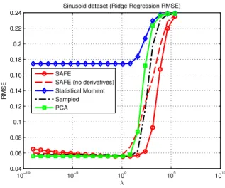
B. The sinusoid dataset
The purpose of the sinusoid dataset is to reproduce a situation in which only an unknown part of the input time series influence the target variable. In mathematical terms, the input time series is defined as follows:
x(t) = sin(tω+δ)
ω ∼ U(0.01,10) δ∼ U(0,2π) while the target variable is computed as
y=
Z 0.7
0.3
x(t)dt=cos(0.3ω+δ)−cos(0.7ω+δ)
ω
Figure 1 shows the results for the sinusoid dataset: it is apparent that, while the statistical moment-based feature extraction is not able to learn a correct model, all the other techniques yield almost the same performances. This is quite unsurprising, since the statistical moment extraction relies exclusively on global features, and is therefore unable to
10−10 10−5 100 105 1010 0.04 0.06 0.08 0.1 0.12 0.14 0.16 0.18 0.2 0.22 0.24
Sinusoid dataset (Ridge Regression RMSE)
λ
RMSE
SAFE
SAFE (no derivatives) Statistical Moment Sampled PCA
Fig. 1. Sinusoid dataset results (average over 500 simulations)
10−10 10−5 100 105 1010 0.05 0.1 0.15 0.2 0.25 0.3 0.35 0.4 0.45 λ RMSE
Ramp dataset (Ridge Regression RMSE) SAFE
SAFE (no derivatives) Moments Sampled PCA
Fig. 2. Ramp dataset results (average over 500 simulations)
select the correct range in the input time series. By analyt-ically inspecting the RMSE results the SAFE methodology yields marginally better results w.r.t. sampling- and PCA-based feature extraction.
C. The ramp dataset
The goal of the ramp dataset is to highlight the advan-tages of including time series derivative information in the extracted features. The input time series is generated as
x(t) = (
n1√2t t <0.5
n1+n2(t−0.5) t≥0.5
n1∼ U(0,1), n2∼ U(1,4),
while the output variable reads
y=n2.
In other words, the slope of the second part ofx(t)(fort≥
0.5) is the target variable. Figure 2 shows the test results for the ramp dataset. As expected, the incorporation of derivative information in the input dataset allows expanded SAFE to outperform the other methodologies.
CONCLUSIONS
In this paper, a novel feature extraction framework is presented for dataset consisting of time series input spaces and scalar target variable. The research is originally moti-vated by real-life datasets representing industrial processes, but the presented results are appliable to any time series-intensive learning environment (such as bioengineering). The proposed methodology, SAFE, derives from a functional learning setting in which the time series input space is reconstructed by means of Gaussian process inference, and the unknown shape function is parametrized as a weighted sum of Gaussian functions. This setup allows for a number of interesting properties, including closed form solution and the possibility of using the extracted information as input for any machine learning methodology. The capabilities of the SAFE methodology have been assessed by means of simulated examples, with the purpose of testing the novel framework against similar techniques. Such benchmarks yield promising preliminary results, as the proposed methodology is able to obtain in general better results than its competitors, including situations where the target output is determined by global features of the input time series.
APPENDIXA
Let G(b, B;x) be the univariate Gaussian probability distribution function of expected value b and varianceB as in (11). By applying derivative rules, it follows that
∂G(b, B;x) ∂x = − x−b B G(b, B;x) (18) ∂2G(b, B;x) ∂2x = G(b, B;x) B2 ((x−b) 2−B) (19)
In the following we consider the theorem proposed in [11] in the special case for whichs=t= 1andQ= 1.
Theorem 4.1: LetA∈Rs×s,a∈Rs,B∈Rt×t,b∈Rt
andQ∈Rs×t. Letx∈
Rtbe an input variable. It holds
that
G(a,A;Qx)G(b,B;x) =G(a,A+QBQ0;b)× ×G(d,D;x)
with D = (Q0A−1Q + B−1)−1 and d = b +
DQ0A−1(a−Qb) Proof of Theorem 2.1. Let
χ= Z ∞ −∞ G(a, A;x)G(b, B;x)dx By applying Theorem 4.1, χ=G(a, A+B;b) Z ∞ −∞ G(d, D;x)dx (20)
Since by definitionR−∞∞ G(d, D;x)dx= 1it holds thatχ=
G(a, A+B;b). Proof of Theorem 3.1 χ = Z ∞ −∞ G(a, A;x)∂G(b, B;x) ∂x dx = −1 B Z ∞ −∞ (x−b)G(a, A;x)G(b, B;x) = −G(a, A+B;b) B Z ∞ −∞ (x−b)G(d, D;x)dx = −G(a, A+B;b) B (d−b)
Since, following Theorem 4.1,
d−b=DA−1(a−b) = A− 1 A−1+B−1(a−b) it holds that −1 B A−1 A−1+B−1(a−b) = − a−b A+B and therefore χ=−a−b A+B G(a, A+B;b). Proof of Theorem 3.2. χ= Z ∞ −∞ G(a, A;x)∂ 2G(b, B;x) ∂2x dx = 1 B2 Z ∞ −∞ G(a, A;x)G(b, B;x) (x−b)2−B dx =G(a, A+B;b) B2 Z ∞ −∞ G(d, D;x) (x−b)2−B dx Since (x−b)2 = (x−d)2 +b2−d2 −2bx+ 2dx and R∞ −∞G(d, D;x)(x−d) 2dx=D it holds that Z ∞ −∞ G(d, D;x)((x−b)2−B)dx=D+ (b−d)2−B and therefore χ = D+ (b−d) 2−B B2 G(a, A+B;b) = (a−b) 2 −(A+B) (A+B)2 G(a, A+B;b). REFERENCES
[1] A. Aizerman, E.M. Braverman, L.I. RozonerTheoretical Foundations of the Potential Function Method in Pattern Recognition Learning, Automation and Remote Control 25, 821-837 (1964).
[2] N. Aronszajn, Theory of Reproducing Kernels, Transactions of the American Mathematical Society 68(3), 337-404 (1950).
[3] H.-J. Dai, Y.-C. Chang, R.T.-H., Tsai, W.-L. HsuNew Challenges for Biological Text-Mining in the Next Decade, Journal of Computer Science and Technology 25(1), 169-179 (2010).
[4] T. Hastie, R. Tibshirani, J. Friedman, The Elements of Statistical Learning. Data Mining, Inference and Prediction., Springer (2009). [5] L. Monostori AI and machine learning techniques for managing
complexity, changes and uncertainties in manufacturing, Engineering Applications of Artificial Intelligence 16(4), 277-291 (2003). [6] G. Pillonetto, F. Dinuzzo, G. De Nicolao,Bayesian Online Multitask
Learning of Gaussian Processes, IEEE Transactions on Pattern Anal-ysis and Machine Intelligence 32(2), 193-205 (2010).
[7] W. Rudin,Real and Complex Analysis, McGraw-Hill (1966). [8] A. Schirru, S. Pampuri, C. De Luca, G. De Nicolao,Multilevel
Ker-nel Methods for Virtual Metrology in Semiconductor Manufacturing, Proceedings of the 18th IFAC World Congress, Milan (2011). [9] B. Scholkopf, A. SmolaLearning with Kernels, The MIT Press (2001). [10] A.N. Tikhonov,On the Stability of Inverse Problems, C.R. (Doklady)
Acad. Sci. URSS (N.S.) 39, 176-179 (1943).