ABSTRACT
This study contains the description of how to use the
contingent valuation methodology for obtaining the
willingness-to-pay information for planning the cost recovery system of a
community water supply in Guatemala. An analysis was made to
identify the weaknesses and strengths of the willingness-to-pay
study for this case. Based on this analysis* recommendations were
made on how to improve and extend these studies to obtain the
TABLE OF CONTENTS
Page
LIST OF FIGURES ... iv
L 1ST OF TABLES ... v
CHAPTER I. INTRODUCTION ... 1
CHAPTER II. DESCRIPTION OF THE CASE STUDY II.1 Site Selection... 6
lI.E Household Questionnaire... 7
II.3 Socioeconomic Characteristics... 9
11.*^ Current Water Situation... 10
11.5 Willingness to Pay for Water Consumption... 12
I 1.6 Willingness to Pay for Connections... 1*^
I 1.7 Explanatory Model of Wi11ingness-to-Pay Bids for Water Consumption. Data Validation... 15
I I.8 Summary... 19
CHAPTER III. PLANNING THE COST RECOVERY SYSTEM Ill.i Required Information... "^ 1 111.2 Water Demand Function... ^2
111.3 General Assumptions... '^4
111.^ Financially Self Sufficient System... '^5
111.5 System Maximising Net Benefits... '^9
111.6 Comments on the Results... 53
111.7 Ranking Function of Projects... 55
I I I . 8 Summary... 57
CHAPTER IV. ASSESSMENT OF THE WILLINGNESS-TO-PAY STUDY IV.1 Strengths of the Wi11ingness-to-Pay Study... 76
IV.2 Weaknesses of the Wi11ingness-to-Pay Study.... SO IV.3 Extension of Wi11ingness-to-Pay Studies... 85
IV.4 Improving of Wi11ingness-to-Pay Studies... 88
CHAPTER V. CONCLUSIONS AND RECOMMENDATIONS. V.l Conclusions... 91
V.S Recommendations... 94
LIST OF FIGURES
Figure
I-l, Schemes of the Bidding Game...
I-S Proportion of Connections vs Water Price....
1-3. Proportion of Connections vs Connection Fee,
II-l. Present Value Net Benefits vs Water Price...
II-2. Net Revenues vs Proportion of Connections..,
Page
. 38 , 39 . 40 . 70 . 71
11.3. Net Revenues vs Time... 7H
11.4 Water Price vs Water Consumption... 73
11.5 Present Value Net Benefits vs Water Price... 74
LIST OF TABLES
Table Page
II-l. Number of Persons per Household... 21
II-S. Education Level of the Head of Household... 22
II-3. Years of Education of the Head of Household... 23
11-^. Occupation of the Head of Households... 2^
I 1-5. Total Household Income... 25
I 1-6. Income of Household Head by Years of Education... 26
11-7. Proportion of Households Using each Water Source... 27
I 1-8. Number of Sources Used in the Dry Season... 27
I 1-9. Distance from Households to each Source... 28
II-IO. Total Monthly Water Use per Household ... 29
II-ll. Per Capita Water Use... 30
11-12. Monthly Household Expenditure on Water... 31
11-13. Monthly per Capita Expenditure on Water... 32
II-l"^. Monthly Household Expenditure on Water as a Percent of HousehoId Income ... 33
11-15. Wi 11 ingnes5-to-Pay Bids for Consumption... 3"^ 11-16. Wi 1 1 ingness-to-Pay Bids for Connection... 35
11-17. Existing Tariff for Guatemala City... 36
Il-ia. Explanatory Model of Wi11ingness-to-Pay Bids for Consumption... 37
III-l. Characteristics New Piped System... 59
III-2. Number of Households Connected as a Function of Water Price... 60
III-'4. Total Annual Revenues... 6H
I 11-5. Construction Cost of the Water System... 63
111-6. Operation and Maintenance Costs... 64
I I 1-7 . Total Annual Costs... 65
II 1-8 . Net Revenues... 66
III-9. Total Economic Benefits... 67
III-IO. Total Net Economic Benefits... 68
OHAPTER 1
INTRODUCTION
It is a common practice of engineers in developing countries
to select 1) the level of service, and H) the price to charge
for new or improved water supply systems, with little input from
the community. This practice frequently results in problems: one
is that households may not use the water system. Different
reasons can account for this, for example, households may not
want the selected level of service, or the prices may be too
high, preventing connections. A second problem is that the costs
of the system may not be recovered. This can result from either
prices that are too high, preventing the connection of households
to the system, or prices that are too low, resulting in
insufficient revenues. For projects in which the number of users
is lower than anticipated and in which costs are not adequately
recovered, the quality of operation, maintenance and service
usually deteriorates, with the result that households may turn
to other sources. Examples of this vicious circle of
deterioration are common (Okun, 1988).
A better basis for selecting the level of service and prices
is needed in order to avoid these problems. This basis should be
aimed at improving the ability of planners and engineers to make
predictions of the level of service that households want to use
Estimation of households willingness to pay for different
levels of service using the contingent valuation methodology
< CVIi) has been suggested as a way to address the problems
discussed above. Whittington? et al. <1987a) after conducting a
field study in Haiti concluded that contingent valuation surveys
may provide valuable information on household willingness to pay
for improved water supply service; they hold promise for helping
CRfTimuni t ies to meet specific cost recovery targetsj to determine
the prices and connection fees to be charged? and to select the
level of service to be provided. Subsequent studies in Nigeria
(Whittington, et al. 198Sa) and elsewhere (Lauria, et al. 1988)
have strengthened the promise of the CVM for selecting
appropriate technologies and designing tariffs. Indeed* the CVM
has been tested for such additional issues as assessing household
attitudes toward their entitlement to piped water supply at
government expense (Whittington, et al. 1988b), and estimating
the implicit value of time spent collecting water <liu,1988).
In the CVM, households are asked directly about their
willingness to pay for a particular level of water service. In
these studies, an interviewer collects information on consumers'
behavior in a hypothetical market. The rationale behind this
methodology is simple: if people say they are willing to pay for
a particular level of service, it indicates that the service is
3
the project. In addition to the willingness-to-pay information}
basic data concerning the household? its socioeconomic
characteristics* and its water use practices are also collected
in these studies.
Application of the CVM in determining willingness to pay for
water is somewhat new. There are uncertainties about whether the
CVM can provide an appropriate basis for determining the level of
service and the price to charge. In principle? a cumulative
distribution function of the willingness-to-pay bids would
indicate the percentage of households that would connect at
alternative prices. However, there is always uncertainty about
the accuracy of the bids. Additionally* the CVM does not directly
produce information about the amount of water that households may
consume at alternative prices* which is also needed for planning
community water systems.
The goal of this project is to evaluate the CVM as a tool
for planning the cost recovery system of a community water supply
case study in Guatemala. Three objectives have been set to
achieve this goal. The first is to plan a cost recovery system
for the case study using willingness-to-pay information to the
extent possible. The second is to assess the strengths and
weaknesses of the willingness-to-pay study using the CVM for
improve the needed information for this case, and to extend such
studies in the future.The task for the first objective includes several steps,
starting with a willingness to pay study using the CVM. This step
includes questionnaire design, interviewer training, and
household surveys. Second, the results from the surveys need to
be analyzed in order to obtain basic information on the
community in such a way that can be used for planning purposes.
From this step, a frequency distribution of household
willingness-to-pay data for connections to the improved system
can be obtained; data validation is also a part of this step.
Finally, the information will be used for planning the cost
recovery system, including the level of service to provide, the
price to charge, the population that will use the improved
system, estimated revenues and cost of the system, financial
requirements, etc. Where data are lacking assumption will be
made.
In accomplishing the second objective, an analysis will be
conducted in order to identify the strengths and weaknesses of
the CVM in producing the information needed for planning.
Distinction will be made between the generic strengths and
weaknesses of the methodology and the specific needs of this
case; the sufficiency and accuracy of the information provided by
The task in third objective is to make recommendations on
how to improve and extend willingness-to-pay studies to obtain
the information needed for planning a cost recovery system for a
communi
ty-This report is organized as follows: in Chapter II, a
description of the case study is provided including site
selection, its socioeconomic characteristics and current water
practices, analysis of the willingness-to-pay data, and the
model for testing the validity of the willingness-to-pay bids.
Chapter III illustrates how to use the willingness-to-pay
information for planning a cost recovery system; the procedures
and assumptions are described in this chapter. Chapter IV
presents the discussion of strengths and weaknesses of the CVM
CHAPTHR II
DESaRIPTlOW OF THE CASE STUDY
II.1. SITE SELECTION.
This study was supported by the CDIi-WASH project (Water and
Sanitation for Health) with funds from the US Agency for
International Development (AID). It started with a reconnaissance
mission to Guatemala in January 1988 to determine whether a
willingness-to-pay study could be conducted in that country.
During this initial visit, different places were investigated as
possible candidates, and contacts were established with the
Regional School of Sanitary Engineer at San Carlos University
(ERIS) to arrange for students and professors to assist with
field work. The conclusion of this mission was that Guatemala
City was a suitable site for this project. In June 1988, a team
of three persons from the University of North Carolina at Chapel
Hill (UNO went to Guatemala to conduct the field work during a
three-week period. This team had the assistance of 12 students
and faculty from the ERIS.
TIERRANUEVA II was one of two places selected for a
wi11ingness-to-pay study. This community of about 600 households
near Chinautla is close to Guatemala City; it is only a few years
7
TIERRANUEVA does not have a piped water system; most of the
water consumed is bought from tanker truck vendors. In addition,
a few private wells and public tanks, temporally installed by the
government, exist in the community. However, most people get
most or all of their water from vendors.
II-2- HOUSEHOLD QUESTIONNAIRE.
The household questionnaire for TIERRANUEVA was developed
and tested during a period of several days. The final version of
the questionnaire began with a statement of the objectives of
the study and the institutions that were conducting it. It was
explained that as a result of the study, an improvement would not
necessarily occur in the water situation in TIERRANUEVA.
Households were given the option not to answer the questionnaire.
The first questions requested basic information such as the
sex of the person being interviewed, the number of adults in the
household, the number of women, and the number of children. The
next section of questions were related to the water sources in
the community, including tanker truck vendors, public tanks,
wells, bottled water, rain water, and neighbors. Households were
asked for each source whether they used it, the amount of
consumption and price in both dry and rainy season, the amounts
8
water had to be carried from the source* reliability of the
source? and the uses that were made of the water.
Next, the questions associated with willingness to pay
were asked. An introductory statement describing the hypothetical
market was read. Each household was told that it would have a
metered private connection at the house providing water with high
quality and in adequate quantity whenever it was wanted.
Additionally? households were told they would have to pay for
every unit of water consumed. Once the introductory statement was
read, the household was asked whether it would like to have
potable water from such an improved system. If the answer was
"No", the CVM was not conducted.
A bidding game was used to determine the willingness to pay.
It consisted of questions about selected prices in order to
identify the maximum range in Quetzales*- per drum*- that the
household would pay for water. Once this range was determined,
the household was asked the maximum price it would pay for a
connection to an improved system. Two versions of the
questionnaire were conducted, one starting at a low price Q
1.0/drum, and the other at a high price Q 1.5 /drum. Figure II-l
shows the two schemes for the bidding game. At its conclusion
* a.5 Quetzales (Q) =1.0 Dollar ($)
9
households were asked if they would pay an additional fee for a connection to the piped system; different amounts were
considered, ranging from $ 24 to *192. Households were told that this fee could be paid monthly during one-year period or all at one time. All the units in the questionnaire were commonly used
by the respondents in their daily activities; volumes were asked
in drums and money in quetzales.
Finally? questions were asked about household
characteristics, including material of the roof, walls and floor; the number of rooms; and whether the household had a toilet. The number of household assets, and the level of education of the head of the house were also asked, plus the sex, occupation and monthly income for each earner in the household. Finally,
households were asked their opinion about the responsibility of government to pay the cost of the water project.
II-3. SOCIOECO»>aDMIC OHARfliCTERISTICS.
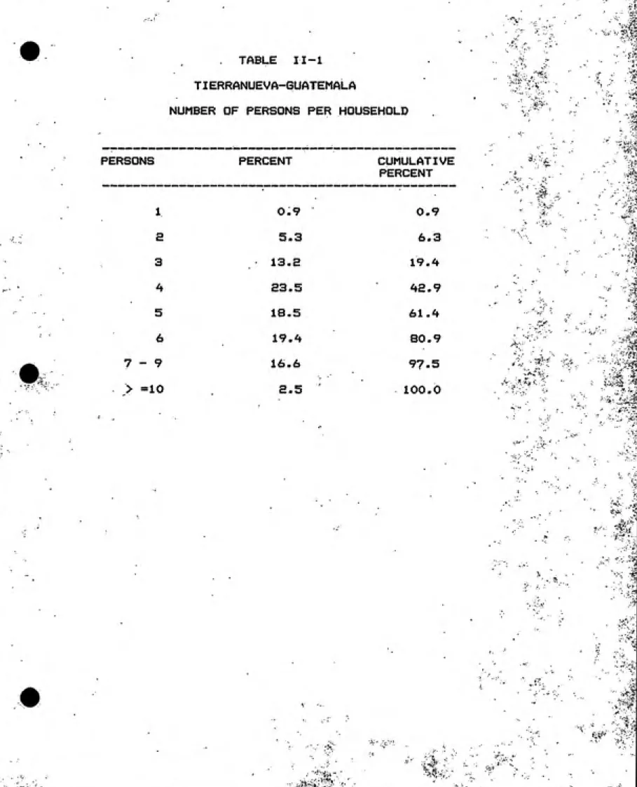
The approximate number of households interviewed in
TIERRANUEVA was 320. The average number of persons per household
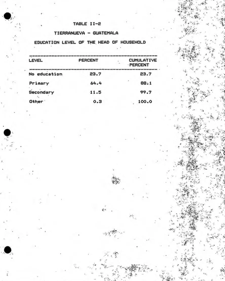
was 5; Table II-l shows that approximately 60'/. of the households have 5 or fewer persons. Table II-E shows that 6'^*/. of the
ͣ
10
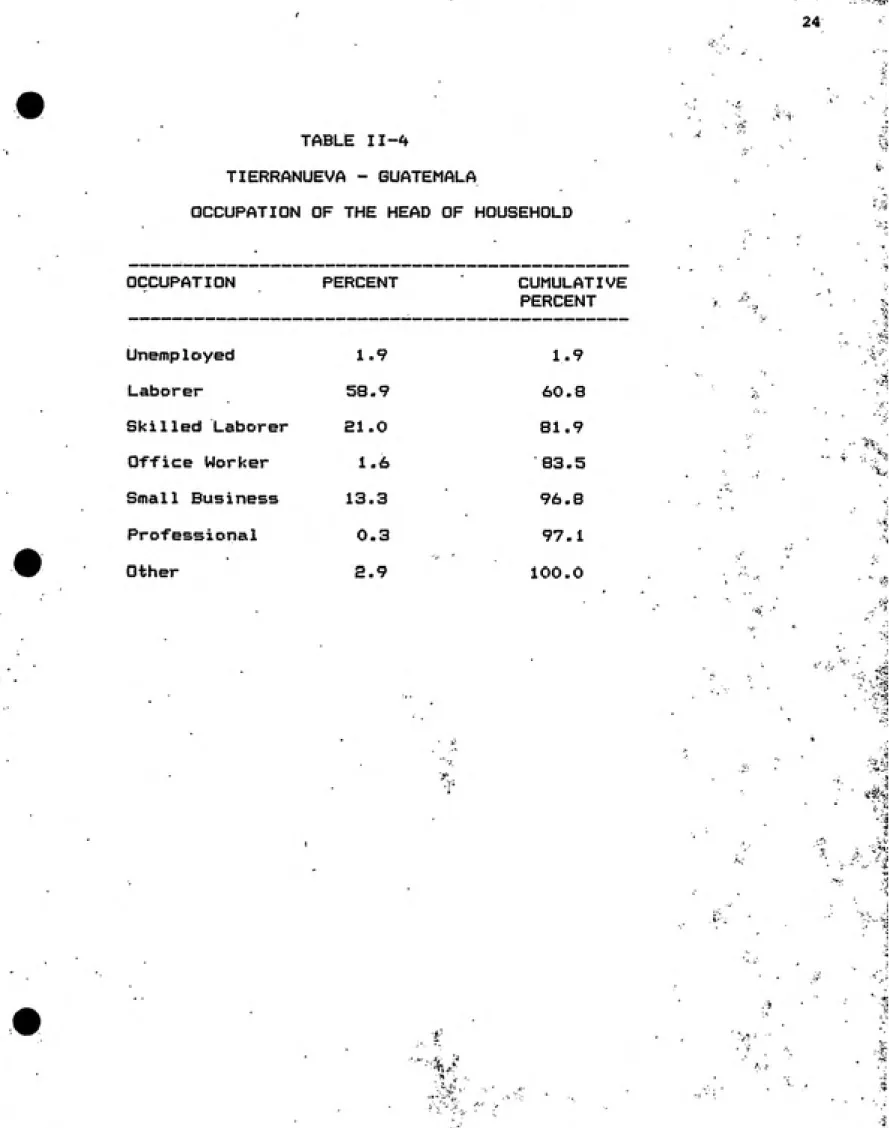
years of education, as shown in Table I 1-3. Almost 60% of the
heads were laborers, and only 0.3V. of them were professionals,
as shown in Table 11-"^.
Average monthly household income was about $100;
two-thirds of the sample had a monthly income lower than $120, and
only 5*/. had monthly income above of $200, as shown in Table I 1-5.
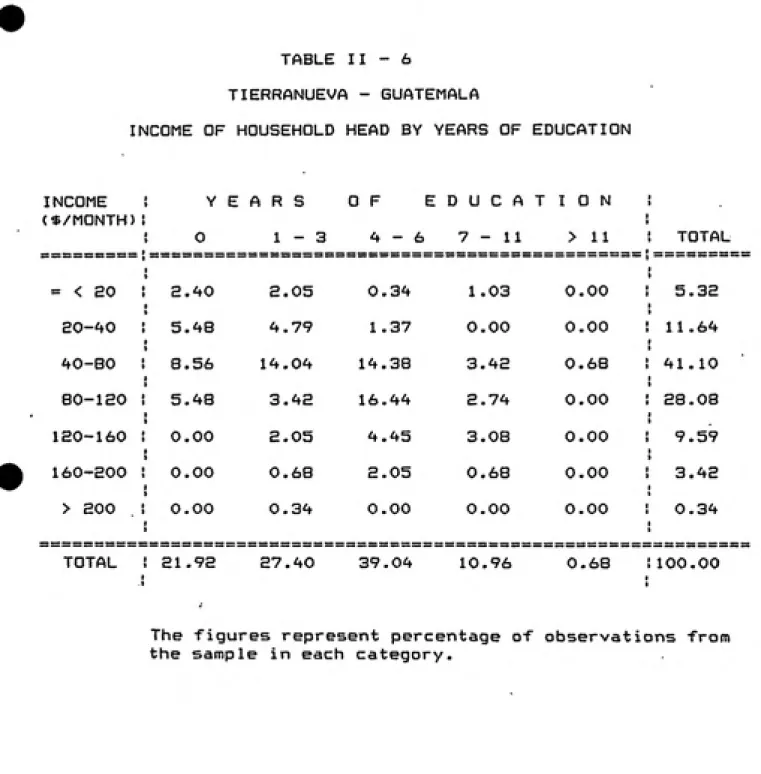
Table 11-6 shows that 100% of the heads of household with no
education earned less than $120 per month, and 75% of those with
three years of education earned less than $80 per month. Almost
60% of all heads of household earned less than $80 per month.
II.A. CORIREINIT yftlBR SITUflTION.
The most important water source in the dry season was
vendors who sold water from tanker trucks; 99% of the households
said that they purchased from them. Even though '43% of the
households used the new public tanks in TIERRANUEVA that were
filled and operated by the government, this source was not very
important for the purposes of this study because it had only been
in operation two weeks at the time of the study. Less than 5% of
the households used wells, 13% purchased bottled water from
vendors, and 20% got water from neighbors, but more as a loan
11
Table I 1-7. In general, more than BOX of the households used 1 or
S sources (vendors and/or public tanks), and 15*/, used three
sources, as shown in Table I I-S.
Water was usually carried only small distances to the house;
tanker trucks delivered it within 10 meters for 70% of their
customers. Fifty percent of the households using the public
tanks had to carry water less than 50 meters, and 70% of the
households that borrowed water from neighbors got it within a
50-meter distance, as shown in Table I 1-9.
The average consumption of water during the dry season from
all sources was about 5.6 cubic meters <cm) per month per
household <hh) or approximately 40 liters per capita per day
(led). Almost half of the households consumed less than 5
cm/month, one-third consumed more than 6 cm/month, and only 7*/,
consumed more than 10 cm/mo, as shown in Table 11-10. Table 11-11
shows water consumption on a per capita basis; 17% of the
households consumed less than 20 led, more than 70% consumed less
than "^7 led, and only E% consumed more than 100 led.
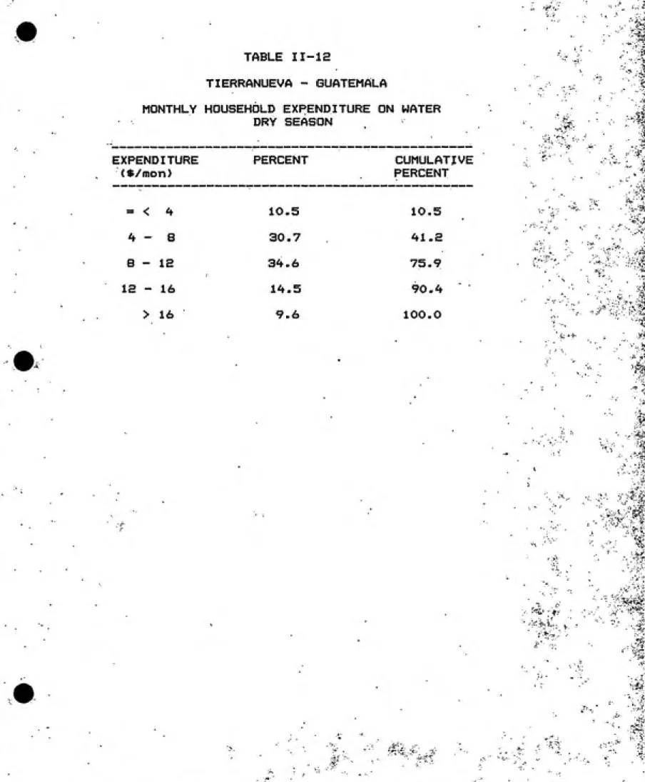
The average household expenditure on water during the dry
season was about ^1.9 per month, which, based on average
consumption of 5.6 cm/month, amounted to an average cost of $1.8
per cm; water from vendors cost $2 per cm on the average. Only
IS
three-fourths spent less than $12 per month, and lOX spent more
than *16 per month, as shown in Table 11-12. On a per capita
basis, more than 20% of the households spent more than $2.8 per
month per person, and only 1^'A spent less than $0.8 per month
per person, as shown in Table 11-13. Table II-l^ shows that only
18*/. of the households spent less than 5*/. of their total income on water, half of the households spent less than 10%, and 10% of the sample spent more than 20% of their income on water.
II.5. WILLINGWESS TO PAY FOR lUlftTER COHiSUMPTION.
The responses of households regarding their maximum
willingness to pay for water were converted to a commodity price basis <dollars/cm). The frequency distribution of the maximum
willingness-to-pay responses is shown in Table 11-15. This
distribution can be used to predict the proportion of households
in the community that will use the new water system at any price
that is charged by the utility. The results show that as water price increases, the number of households that will use the
improved source decreases. For example, if the price is set to $2
per cm < the current price paid to vendors), only '^9% of the households said they would use the new system; if the price is
$l/cm, almost three-fourths of the households would buy water
from the improved system. The average willingness-to-pay bid was
13
vendors and equal to the average cost that all households are
currently
paying-The results in Table 11-15 are useful for planers because
they describe the coverage that the new water project would have
at alternative prices. This information is used in Chapter III to
plan the cost recovery system for TIERRANUEVA. In order to
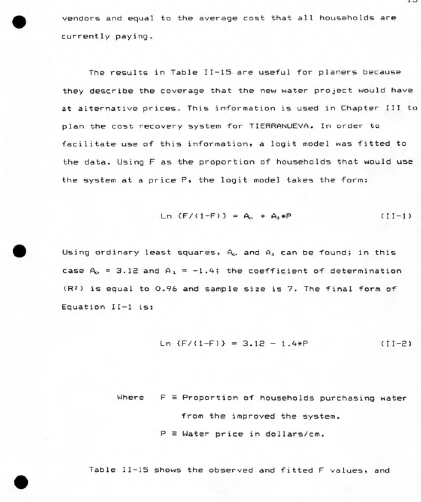
facilitate use of this information, a logit model was fitted to
the data. Using F as the proportion of households that would use
the system at a price P, the logit model takes the form:
Ln <:F/(1-F)> = A,,, + A.i»P (II-l)
Using ordinary least squares, A^;. and Ai can be found; in this
case Ac, = 3. IS and A j. = -l."^; the coefficient of determination
<R2) is equal to 0.96 and sample size is 7. The final form of
Equation II-l is:
Ln <:F/<1-F)> = 3-12 - l.^*P (II-E)
Where F = Proportion of households purchasing water
from the improved the system. P = Water price in dollars/cm.
14
Figure II-l shows the proportion of households that would use the
system at each alternative price.
II .6 tUILLIIMGNESS TO PAY FOR COMNECTIONS. •
In addition to the bidding game for determining the maximum price a household would pay for water from the improved system, each respondent was asked whether he/she would be willing to pay an additional amount of money in order to connect to the piped system. The procedure used was different from that for
determining the willingness to pay for consumption. Various
connection fees were chosen in advance, and the interviewer
selected one randomly; the household was then asked if it would still connect to the system given the option to pay the fee
monthly during the year or all at one time.
Results are shown in Table 11-16; as the connection fee
increases, the proportion of households that would connect to the new system decreases. For example, if the fee were $'^8, the proportion of households that would connect is 90'/.; however, if the connection fee were increased to $1S0, the proportion would decrease to 60*/. Most of the household were willing to pay
15
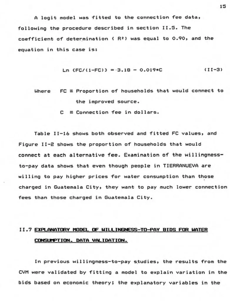
A logit model was fitted to the connection fee data, following the procedure described in section II.5. The
coefficient of determination ( R^) was equal to 0.90, and the
equation in this case is:
Ln <FC/<;i-FC)> = 3.18 - 0.019-k-C <II-3)
Where FC = Proportion of households that would connect to the improved source.
C = Connection fee in dollars.
Table 11-16 shows both observed and fitted FC values, and
Figure I 1-2 shows the proportion of households that would
connect at each alternative fee. Examination of the willingness-to-pay data shows that even though people in TIERRANUEVA are willing to pay higher prices for water consumption than those charged in Guatemala City, they want to pay much lower connection fees than those charged in Guatemala City.
11.7 EXPLfflNMiTORY MODEL OF MILLI><l»ESS-TO-PAY BIDS FOR WATER CONSUMPTIONI. EJATft VALIDATIONI.
In previous willingness-to-pay studies, the results from the CVM were validated by fitting a model to explain variation in the
16
model represent both household and source characteristics. It is
assumed that if much of the variation in the willingness-to-pay
bids can be explained by the model* the bids were not given at
random. In other words* these bids would constitute valid
information that could be used with confidence for planning
purposes.
A multiple regression model with variables representing
household and source characteristics was fitted to the
TIERRANUEVA data. The units of the dependent variable were
Quetzales per drum. Two variables representing source
characteristics were included in the model. The first? called
NEAR> was the distance from the house to where the water was
delivered by the tanker truck vendor. If the vendor delivered
water within 10 meters of the house, NEAR = 1, and NEAR = 0 if
the distance exceeds 10 meters. The sign of the regression
coefficient of NEAR is expected to be negative since households
with small distances to the source are expected to bid less than
those having to carry the water long distances.
The second variable was the quality of water from the
present sources used by the household. This variable, called SAL,
has value 1 for households using bottled water and 0 otherwise.
It is expected that households using bottled water are
dissatisfied with the quality of water from the main source
17
SAL was positive.
Three variables associated with household characteristics were included in the model- The first was INGR, a variable that
indicates whether household monthly income was higher than *200;
for income less than $200, INGR = 1 and 0 otherwise. Households
with high income were expected to bid high prices, which
resulted in an expected negative coefficient for INGR. The
second variable related to the education of the head of the household (ED). This was a dichotomous variable with value 1 if
the head had not more than two years of education and 0
otherwise. The expected sign of the coefficient of this variable
is negative. The third household variable was the type of
occupation of its head (WORK); this variable had a value of 1 if
the head was a professional and.0 otherwise. The expected sign
for the coefficient of this variable was positive.
Two other variables were included in the model. A dummy
variable was used to test starting point bias in the bidding
game (ZBID); if the game started with a high price, ZBID had
value 1 and O otherwise. Finally, a variable was included to test
whether the bids from female respondents were different from
those of males (FEML); if the respondent was female, FEML was
equal to 1.
IS
The level of significance of the model is only 10%> and its
coefficient of determination (R2) is very low (0.1). All the
coefficients of the explanatory variables in the model had the
expected signs? but most of them are statistically insignificant,
suggesting that the variables do not explain very much of the
variation in the bids. The variable NEAR is significant at about
10*/»; water quality was insignificant) income and education are
roughly significant at a 20*/, level; and occupation is
insignificant. The model? therefore, has little predictive power;
it does not explain very much of the variation of the bids,
making uncertain whether the bids can be used with confidence for
planning purposes.
This process of validation corroborates what can be seen
from an examination of the bids. Half of the households said
they would not use the new system if the price were as high as
*2/cm, and only 75*/. would use it if the price were set to $l/cm.
However, most households presently pay about *E/cm to vendors
which would make it advantageous for them to connect to the new
system at any price up to this amount if they though that water
and service quality would be improved. Different reasons might
explain the low bids. Perhaps the benefits from the new project
were doubted or not well perceived, or the households were
influenced by the low prices people are currently paying in
did not know how much they were presently paying. In any event*
the bids raise a question with practical implications: what
should be done in cases like TIERRANUEVA, where after conducting
the willingness-to-pay study, the data appear to be highly
questionable?
ii.B.SLumgmr.
The willingness-to-pay study provided basic information on
household and source characteristics. The willingness-to-pay
bids for a connection to the new system were presented in a
frequency distribution that shows the percentage of households
that would use or connect to the new system at different prices.
In addition, data were collected on the initial amounts that
households were willing to pay for a connection. Logit models
were fitted to the willingness-to-pay bids.
The results indicate that people in TIERRANUEVA are willing
to pay higher prices for water from an improved system than those
paid in Guatemala City. The situation is reversed, however, with
respect to connection fees: they do not want to pay as much as
people in Guatemala City have to pay for being connected to the
piped system.
. . ao
past studies. A multiple regression model was developed to
explain household willingness to pay for water from a new piped
system. The level of significance of this model was very weak?
which makes uncertain the validity of the willingness-to-pay bids
for planning purposes. This result raises questions about the
ability of the CVM to obtain accurate data; it also casts doubt
21
TABLE ir-l TIERRANUEVA-GUATEMALA
NUMBER OF PERSONS PER HOUSEHOLD
PERSONS
----PERCENT
CUMULATIVE-»..«—_-«
PERCENT
0,9 0.9
5.3 6.3
13.E 19. ''+
23.5 h2.9
IS.5 61 . H
1 9 . H SO. 9
1
s 3 4 5 6
9 16.6 97.5
22
TABLE II-E
TIERRANUEVA - GUATEMALA
EDUCATION LEVEL OF THE HEAD OF HOUSEHOLD
LEVEL
No educati o n
PERCENT
E3.7
CUMULATIVE PERCENT
S3.7
Pr imary 6h . ^\ as.i
SecondaTV 11.5 99.7
23
TABLE 11-3
TIERRANUEVA - GUATEMALA
YEARS OF EDUCATION OF THE HEAD OF HOUSEHOLD
YEARS PERCENT . CUMULATIVE
PERCENT
0 S'+ . 0 BA . 0 1 3.s a?.3
a 10.H 37.7 3 i3„3 51 „0
^ 10.1 61.0
5 6.S 67,9
6 SO.8 88.6
7 1.6 90.3 8 S.9 93.E 9 3,9 97„1 10 1.0 98,1 11 1.3 99.
A-ͣ
24
TABLE II-^+
TIERRANUEVA - GUATEMALA
OCCUPATION OF THE HEAD OF HOUSEHOLD
OCCUPATION PERCENT CUMULATIVE PERCENT
25
TABLE I I-5
TIERRANUEVA - GUATEMALA TOTAL HOUSEHOLD INCOME
INCOME PERCENT CUMULATIVE
ͣ
*/month) PERCENT
= <:: SO . 1 .. 0 1 »C!
20- 40 6.3 7,2 40- SO 34,9 42.i 80-120 25.7' 67,8 120--160 16 „ 4 84. E
26
TABLE II - 6
TIERRANUEVA - GUATEMALA
INCOME OF HOUSEHOLD HEAD BY YEARS OF EDUCATION
INCOME ! (*/MONTH)1
YEARS 0 1-3
OF E
4-6
DUCAT
7-11
I 0 N
> 11 ! TOTAL
= < EO ! 2.40 2.05 0.34 1 .03 0.00 i 5.32 20-40 1 5.48 4.79 1 .37 0.00 0.00 ! 11.64 40-BO I 8.56 14.04 14.38 3.42 0.68 I 41.10 80-lEO 1 5.48 3.42 16.44 2.74 0.00 : 28.08 120-160 ! 0.00 2.05 4.45 3.08 0.00 1 9.57 160-200 : 0.00 0.68 2.05 0.68 0.00 1 3.42
> 200 ! 0.00 0.34 0.00 0.00 0.00 1 0.34
TOTAL 21.92 27.40 39.04 10.96 0.68 :100.00
The figures represent percentage of observations from
27
TABLE I 1-7
TIERRANUEVA - GUATEMALA
PROPORTION OF HOUSEHOLDS USING EACH WATER SOURCE DRY SEASON
SOURCE •/. OF HOUSEHOLDS USING SOURCE
Tanker Truck Vendors 99 Public Tanks ^^3 Wells 3 Bottled Water 13 Neighbors 19
TABLE I I-8
TIERRANUEVA - GUATEMALA
NUMBER OF SOURCES USED IN THE DRY SEASON
SOURCES PERCENT CUMULATIVE PERCENT
1 37.9 37.9
3 14.6 98.8
ͣ
28
TABLE 11 -• 9
TIERRANLIEVA - GUATEMALA
DISTANCE FROM HOUSEHOLDS TO EACH SOURCE DRY SEASON
DISTANCES TANKER TRUCK PUBLIC WELLS BOTTLED NEIGHBORS
(m) VENDOR TANKS WATER
< %) <%) •; %) .: v: i%)
I.)
0 1 - 10 11 --51 - 100 101 - aoo
>soo
E'3 37
0.^+
1„1 12,8
3S„3
£'3. ^t 16.0
8,5 lOOnO
100.0
4 7.,6
11.9
TABLE 11-10
TIERRANUEVA - GUATEMALA TOTAL MONTHLY WATER USE PER HOUSEHOLD
DRY SEASON
29
QUANTITY
<CM/MONTH)
PERCENT CUMULATIVE
PERCENT
1 - B e - 3 3 - <;+
o
8 ->
8 10
10
t.. ti ^i „6
11. 3
16-5 10. a 19 .4 £1. 5 6. 7 7. 4
IS.3
3i^.9 -4-5 „ 1
hH .'+ 85.7
92-,6
30
TABLE 11-11 TIERRANIJEVA - GUATEMALA PER CAPITA MONTHLY WATER USE
DRY SEASON
QUANTITY PERCENT CUMULATIVE
.;ipd) PERCENT
= •::: 7 1.1 1.1 7 ~ SO 16,3 ͣ 1l.7.'-> RO - 33 30,9 hS.S
33 - h7 ES,-^ 71 „ 6 47 - 67 17 . 7 £i9 , h
67 ͣͣ•ͣ• 100 8„9 9Sna
3]
TABLE II-IS
TIERRANUEVA - GUATEMALA
MONTHLY HOUSEHOLD EXPENDITURE ON WATER
DRY SEASON
---EXPENDITURE PERCENT (*/niDn)
= < 4 10,. 5
4 - 8 30, 7
8 - IE 34 - 6
IS - 16 14.5
> 16 9.,6
CUMULATIVE PERCENT
10.5 41 .2 75.9
32
TABLE 11-13
TIERRANUEVA - (BUATEMALA
MONTHLY PER CAPITA EXPENDITURE ON WATER
DRY SEASON
EXPENDITURE PERCENT CUMULATIVE < * /• MO/CAP IT A ) PERCENT
< = 0.8 13.t> 13.6 0 .8-1.6 30 . 3 H-3 ., 9 1 .6 - S.8 35.1 73.9 S. S ~ H . O 1H . 5 93 , '--i
33
TABLE 11-14
TIERRANUEVA - GUATEMALA
MONTHLY HOUSEHOLD EXPENDITURE ON WATER AS A PERCENT OF TOTAL HOUSEHOLD INCOME
EXPENDITURE PERCENT CUMULATIVE (!4 OF INCOME) PERCENT
ͣ
:ͣͣ = P P q p '-5
a -- 5 15,,3 . 17„7 5 -- 10 3E. 1 h9„3 10 - 15 Eg.8 72,6
15 -ͣ- 20 17 „2 89.8
34
TABLE II - 15 TIERRANUEVA -- '3UATEMALA
WTP BIDS FOR CONSUMPTION
P PERCENT F F RANGE CUMULATIVE FITTED
(*/CM) (!4) (/;) <%)
0.0-0,50 'i^
0.50--0-75 6
0„ 75-1,00 17
1.00-2.OO SA
2.00-3.00 2S 3,OO-H.00 10
'+.00-5,00 9
> 5.00 a
96 92 90 89 73 85 49 58
SI 25
35
TABLE II -- 16
TIERRANUEVA - GUATEMALA WTP El IDS FOR CONNECTION
FC FC
CONNECTION HOUSEHOLDS THAT FITTED
FEE WILL CONNECT VALUES
< $) < %) (% >
S^ 95 9'+
^8 88 90
7a 86 86
96 86 79
120 59 70
l-^'t 53 60
168 42 43
36
TABLE II - 17
TIERRANUEVA - GUATEMALA
EXISTING TARIFF FOR GUATEMALA CITY
CONTRACT AMOUNT < PAJA)
QUANTITY (CM/MO/HH)
MONTHLY COST
<*/MO/HH)
CONNECTION FEE
< *)
1/3 20 0.8 140
1/a 30 a.i E10
37
TABLE 11-IS
TiERRANUEVA - GUATEMALA
EXPLANATORY MODEL OF WTP BIDS FOR CONSUMPTION
VARIABLES PARAMETER STD.
ESTIMATE ERROR t PROB.
Intercept. 1 .09E 0.104 10. 51 < 0.01
INGR -0.099 0.075 -1.33 0.19
ED -0.097 0.08 E -1.18 0 „ S4
WORK 0 . 013 0.023 0.57 0.57
ZBID 0.158 0.074 S. 15 0.03
FEML 0.057 0. lOtj 0.54 0 .59
SALV 0.086 0.106 0.81 0.4E
NEAR -0.128 0. 106 -1.65 0. 1
SOURCE df
ANOVA
ms PROB
MODEL
ERROR TOTAL
7 187
194
3 48
51
0.43 0. S5
1 .9 0 .07
38
SCHEMES FOR THE BIDDING GAME FIGURE II-l
LOW STARTING POINT
^A/OULJ) YOU
PAY Q.O
HIGH STARTING POINT
X^OULD You
PAY 3.0
39
•
PROPORTION OF CONNECTIONS VS PRICERGUf?E !(-2 {it I D U z z 8 D.dS -4 D.9 d.«5 d.e -\ J «_l ^-i^--^ ^^<I-. k. '^s... '"---__ fl ͣ v • ͣ --.. 2 or 0 a 0 or &. d.7S 0.7 -'' X ^ r1 «& "'-ͣ ͣ •.._
n Aft —
.
•
n.ao -| , } ( ! ( J } ( \ \ 1 J , , j ) j 1 0,1 0-.3 0»5 0.7 O.y 1.1 1.3 1.5 1.7 1.9
40
«•
z
IX Z
i
I S
PROPORTION OF CONNLOTIONS VS FEE
figure: 0-3
uu
-B-_
.__^
""--__^
B-.._ "ͣ
--ͣ
-^qH
'ͣͣ--.
'ͣ-._
^n -^ ͣͣ
-,-7D -'
'ͣ--w.
X
ͣ
•ͣͣ-1
•-,
-13
%n
-ͣ
'-ͣ. n
40 60 80 100 120 140
CONNEcTiOM FEE (COLLARS)
CHAPTER III
PLfllWING THE COST RECOVERY SYSTEM
III.l. REQUIRED INFORMATION.
Planning of" the cost recovery system is based on the calculation of revenues and cost. For example, when financial self sufficiency is required, revenues have to be at least equal to the total cost. The design of the cost recovery system needs to provide an adequate balance between costs and revenues over
the project life. This balance depends on the accuracy and
availability of information for cost and revenue calculation.
Once the level of service and the type of system have been decided, the cost of the project depends on its capacity, which
is usually the rate of water consumption in the last year of the
design period, assuming that demands increase over time. Revenue
calculations are based on water consumption at the household level, the number of households using the improved system, and
the water price.
The prediction of water consumption and its variability over the project horizon play a key role in the determination of both revenues and costs. Prediction of the number of households
other words? when each household was interviewed} it gave a value
to its perceived benefits of connecting to the improved system. If the water price is set equal or lower than the
willingness-to-pay bid} the household will use the new system. This information is shown in Table 11-15 in which for each alternative price» the
proportion of households that would use the system is shown. Recall that equation II-2 is the result of fitting a logit model to the data in Table 11-15.
No information was collected on the amount of water each household would purchase at alternative prices. Although there is
plenty of information on current water consumption is not enough to develop a complete demand function. Hence, assumptions need to be made about water demand, which are in section III.E. This
function plays a key role in the design of the cost recovery
system.
The number of households that will connect to the new system and the water demand function represent the starting conditions for project planning. The extent to which this information can be extrapolated into the future is discussed in Chapter IV.
111.2. yffltTER DEMAND FUWCTIOWI.
A3
existing consumption can be used to estimate demand. First>
assume an exponential relationship between water price <P) and
water consumption (Q) of the type:
P = K*EXP(M*Q) <III-l)
In this equation the parameters K and M are unknown. Two
points on the demand curve are required in order estimate these
parameters.
Recall that present average water consumption in the dry
season is 5.6 cm/month per household? and the average household
expenditure is *1.8/cm. Since households in TIERRANUEVA did not
have to spend much time carrying water, it is reasonable to
assume that these figures represent the economic cost of water.
In other words? these values define a point on the water demand
curve. For the second point? recall that more than 90*/. of the
households said they would use the improved source at a price
between *0.5 and $0.75 per cm (see Table 11-15). Assume that at
a price of *0.60/cm, per capita consumption would double to Ih
led (11.'^ cm/month/hh). Using these two points in equation III-lj
the values for the unknown parameters are K=5.2 and ti=-0.19. The
final demand equation is:
P = Water price (dollars/cm).
Q = Average water consumption by connected
households <cm/month/hh).
For equation III-S, the price elasticity of demand ( t ) is
given by the equation:
T = - 5.86/ Q
Considering a price range between $0.6 and $1.5/cm, demand
is inelastic? varying from -0.8 to -0.6? which seems reasonable.
III.3. EENERAL AS^iMPTIONS.
For planning the cost recovery system, additional
assumptions concerning system characteristics, project cost, and loan conditions are needed; the general assumptions used in the analysis of this chapter are listed below.
1. The household water demand function is given by equation 11 1-2; this function is assumed to be constant throughout the
project horizon.
45
hor i zon.
3. The average current water consumption is 6 cm/month/hh.
4. The average current water expenditure is 10 do 1lars/month/hh. 5. The income elasticity of demand zero.
6. Planning horizon equals 20 years.
7. Population growth equals 3 '/. per year.
8. Amortization period of the loan equals SO years.
9. Discount rate 10% per year.
10. Construction of the new project occurs at time zero.
11. There is no difference between prices and true "opportunity
costs".
IS. A same price for water will be charged to all users.
13. Construction costs of the project can be estimated using the software COSTEVAL (Gallagher and Lauria,1988).
l*^. Characteristics of the water system are given in Table III-l 15. Annual operation and maintenance costs are estimated as 50%
of annual debt service.
111."%. FIWIflilMCIflO-Y SELF SUFFICIENT SYSTEM.
Assume the utility wants to achieve financial self
sufficiency for the system. This requires that the present value of total net revenues over the project horizon be equal to zero.
Because there is no subsidy, the utility needs to determine the minimum water price that would generate enough revenues to cover
-^6
Min Water Price = P dollars/cm
Subject to:
Present Value of Net Revenues =0
i) Model Solution. For solving this problem? the following
procedure will be used: a value will be given to the variable water price (P^). Based on this price, the projected water
consumptions revenues and costs will be calculated for each year
of the planning horizon. The streams of revenues and costs will be discounted to present value, and if net present value is not
zero, a new value will be assumed for P». until the solution is
found.
ii) Revenues from the new project can be calculated knowing
the number of households using the improved source, water price,
and the water consumption per household. For a given price P».
dollars/cm, a proportion F^ of the existing households would use
the piped system, and the water consumption would be Q* cm/month.
The values for F^ and 0* are given by equations II-S and III-H.
The annual revenues from each connected household can be written;
^1
Considering that a proportion F,, of" the existing N».
households would use the new system, the total revenues in any
year i from the entire community are:
TRi = R;, *Ni *Fv = N^ *F:t *Pi *a^*ia dollars/year.
TRi = N*< 1+9) ^*Fi.*Pi.*Qi*lE dollars/year. <III-3)
Where F^ = Proportion of households using the new system
Qi = Monthly water consumption (cm/household) Pi = Water price <dollars/cm)
N = Initial number of households in the community
Ni = Number of households in the community in year i
6 = Annual population growth rate, decimal.
Table III-E shows the number of households that would use
the new system over the project horizon at alternative prices. This information is converted to yearly water consumption in Table I I 1-3. Total annual revenues and present value revenues are shown in Table
III-*^-iii) Construction cost of the project for different prices
<i.e. different capacities) is estimated using Costeval. The
results are shown in Table I 11-5. In general, the construction
cost function in equation III-4 for the project fits well < R2=
Where
COST = Construction Cost, $1000. CAPACITY = Maximum daily design flow
including SO */. losses, cmd
48
O A*?
COST = 3.SO * CCAPACITYl <III-'^)
The operation and maintenance cost is calculated using
equation III-4. The required flow for any year is used in this
equation to calculate the construction cost of the system that
would supply that flow; this value is annualized, and 50*/. of it
is assumed to be the operation and maintenance cost for that
year. Table I 11-6 shows the annual operation and maintenance
costs throughout the project horizon. Total annual costs are
shown in Table III-7.
iv) Results. Annual net revenues and present value of net
revenues are shown in Table III-8. According to this table and
Figure III-l, net revenues over the project horizon are close to
zero when the price is set at about * 0.60 per cm. Lower values
generate losses while higher values generate profits. When the
water price is * 0.60 per cm, the proportion of connected
49
Table III-5). This project would generate a revenue surplus in
the ninth year (Figure III-2); its per capita cost based on
present population is $ 123, and based on the design population
it is *68 per capita.
These results indicate that the water price that allows the
utility to achieve financial self sufficiency is $0.60 per cm.
Lower prices would not generate enough revenue to cover total
costs.
III.S. SYSTEM MAXIMIZIIMG NET BEWEFITS.
If this project were to be financed by international
institutions, such as the Interamerican Development Bank or The
World Bank, its feasibility would have to be shown in terms of
its economic benefits. The utility would need to make an
analysis showing that the size of the system and its price,
correspond to conditions in which economic net benefits are
maximized (i.e. economic efficiency is achieved).
The problem in this case is toi
Maximize Net Benefits = 2 (III-5)
50
Subject to:
System Capacity > Water Demands for SO
year-planning horizon.
i ) Model Solution and System Costs are the same as those described in Section III.'^.
ii) Total Benefits from the new project for each household
can be calculated using the household water demand function
(equation I 1-2). Before connecting to the new system? each
household was consuming 6 cm/month and paying on the average
1.66 dollars/cm. Total average water expenditure was close to 10
dollars/month. After connection, households will start paying P^
dollars/cm and increase consumption to Q.,. (see FIGURE III-A-).
Hence, total benefits have two parts: the first 6 cm/month
consumed "represent a substitution of public for privately
supplied water, and the benefit is the aggregate domestic value
of resources saved by the substitution" (Powers, 1978); the
second part of the benefits is associated with increased water
consumption beyond the amount of water previously purchased from
vendors.
The total value of the monthly benefits per household (tmb),
51
tmb = 6*1.66 + Area under demand curve between the levels of consumption 6 and Q j. cm/month.
rQ=cPQ=Qj.
tmb =10 + L , 5.S*EXP(-0.19*Q) dQ dollars/month
The first term <10 dollars/month) is the amount of resources
saved by the substitution. The second term is the benefits for
the increase in consumption as a result of the lower price.
If at the price Pj. a fraction F i. of the total number of
households N connect to the improved source? the total yearly
benefits ( TB». ) for the entire community are:
TBs. = 12* N * F J. *tmb
Considering that every year the number of households in the
community will be different, and the proportion of households
connecting to the piped system is assumed to be unchanged for a
given price, benefits for year i are:
TBi = 12*N*(1+0)^*F*tmb <III-6)
Present value total benefits <TB) over twenty years of the
52
TB = ^=T^^ TB:,*PWFi. 3
TB = i:^^'^C12*N*(l+ e)^*F*tmb*PWFi 3
1 = 1TB = 12*N*F*tmb* t"^^*^ C < 1-<- 9)^* PUF^ 3 <III-7)
1 = 1Where
N = Initial total number of households in the community.
F = Proportion of households connecting at a given price.
This value is assumed constant over the SO years,
tmb = Total monthly benefits per household connected to the
piped system(do 1lars/month).
PWFv = Present worth factor for year i
9 = Annual population growth rate, decimal.
Table I 11-7 shows the annual economic benefits and present
value of total benefits .
iii) Results. From the information in Table III-IO and
Figure III-5j it can be seen that the maximum value of net
economic benefits <*655j000) is obtained when the water price is
set to * 0.30 dollars/cm; net benefits increase as the
proportion of connected households increases to 94 '/., the value
53
expected because of the shape of the water demand curve. The
project would never generates a revenue surplus (Figure III-3).
The required capacity of expansion for a design period of 20
years is 961 cm/day, and the construction cost is * '^ITjOOO. The
per capita construction cost based on the present population is
$139j and it is $ 77 per capita based on the design population.
111 .6. COMnOHITS ON THE RESULTS.
The results of these two case are summarized in Table
III-11. Where it can be seen that:
1) The price that maximizes present value net benefits is
half of that required to achieve financial self sufficiency.
S) If the water price is set to maximize present value net
benefits a subsidy would be required in order to have sufficient
revenues to cover total costs.
3) If the water price is set to achieve financial self
sufficiency* total net benefits would not be maximized. The
decrease in net benefits is a measure of the cost to society for
selecting a price <* 0.60 doll/cm) different from that in which
economic efficiency would be achieved.
54
decreases slightly when the price is set based on financial self
sufficiency,
5) If the price were to be set based on the net benefit
maximization scheme* households would pay 45 'A of what they are
currently paying and would consume S.5 times more water than
their present consumption.
6) If the price were selected based on financial self
sufficiency? households would pay 68 % of what they are paying
now and would consume almost twice as much water.
7) The size of the system to achieve economic efficiency is
25*/. larger than that required for financial self sufficiency.
8) If a single price is charged so as to cover cost, it
should be equal to *0.60 /cm. At this price, no profit would be
made. At any price higher than *0.60/cm> the price that
consumers are willing to pay is higher than average cost, so in
this range, profits would be made. If the price is set lower than
0.60 per cm, the price that consumers a.rG willing to pay is
lower than average cost, so in this range, losses are incurred.
At this point several questions can be asked. Should the
government provide a subsidy equal to 60*/. of the construction
55
efficiency is obtained ? or should the price be set higher so
that revenues can cover total costs and achieve financial self sufficiency of the system? Obviously* these questions cannot be answered without more information on other factors* such as the
availability of subsidies from the government and the existence
of other projects competing for them.
III.7. RANKING RJMCTIOW OF PROJECTS.
The required cost recovery scheme can be selected depending
on the availability of subsidies from the government.
1) First, assume that no subsidy is available. In this case,
the highest level of service should be selected that the community is able to pay for. This option implies that
Revenues > Total Costs
Under this constraint, the water price should be set to $0.60 per cm so that revenues will cover total costs.
If this criterion is used, communities with low willingness
to pay would probably never get an improvement in their water
system because there is no level of service that would meet the
56
S) If there is a subsidy from government and if the only
water project is the one for TIERRANUEVA, the system should be
designed to maximize net benefits. In this case, the water price
should be set to $0.30 per cm.3) If subsidies are available from government but there are
several projects competing for them, the question is whether to
subsidize the TIERRANUEVA system, knowing that if the price is
set to *0.60/cm, more than 90*/. of the households would use the
system, and it would be financially self sufficient. In this
case, a marginal analysis needs to be made; that is, the
government should subsidize the TIERRANUEVA project if the
additional net benefits from each dollar of subsidy are greater
than the net benefits from each dollar of subsidy from other
projects. Considering the present case, additional benefits from
selecting the system maximizing net benefits instead of that in
which financial self sufficiency is achieved, are equal to
$68,000 (655,000-587,000) and the required subsidy is *25E,000;
57
III .8. SUTOTftRY.
Even though no information was collected on water
consumption from the new system, the existing data on current
water consumption and the frequency distribution for consumption
enabled development of an approximate water demand function.
In planning the cost recovery system for TIERRANUEVA, the
CVM provided information on the proportion of households that
would use the improved source, which, together with the water
demand function, facilitated the calculation of revenues. Yearly
water consumption and capacity of the system were the inputs
required for calculation of costs.
Although it is uncertain whether the willingness-to-pay bids
for consumption are valid, their frequency distribution as given
by equation II-E was used for planning the cost recovery system
for TIERRANUEVA. The information on willingness to pay an initial
connection fee to the new system suggested that people in
TIERRANUEVA did not want to pay it. This suggests that in this
case, it would be better to recover costs only through water
tariffs and not through initial fees.
The cost recovery system for the TIERRANUEVA water project
was planned considering two different conditions: financial self
sufficiency and net benefit maximization. In deciding which case
58
to consider requires taking into account existing policies
59
TABLE III-l. TIERRANUEVA. GUATEMALA CHARACTERISTICS NEW PIPED SYSTEM .
BASIC PARAMETERS
i) MAXIMUM DAY/AVERAGE DAY PEAKING FACTOR = 1„5 E) MAXIMUM HOUR/AVERAGE DAY PEAKING FACTOR== S.5
3) WATER SYSTEM COST CONTINGENCY = E5% ^) WELL SOURCE
Capacity each new well --SOO cmd
Well depth = 150 m Well diameter = 15 mm
5) PRESSURE TRANSMISSION MAIN Required length = 1000 m
Ma>; allov-jable velocity ~ 1.5 mps 6) CHLORINATION
E>: ist ing capac i ty - 0
7) PUMPING STATION
Existing capacity ~ 0
8) STORAGE TANK
Existing csipcicity = 0 Detention time •ͣ= 0.S5 days 9) WATER DISTRIBUTION NETWORK
Existing number of connections = 0
Connection cost = 30 doliavrs
EXisting Isngth = 0
60
TABLE 111-2. TIERRA NUEVA. GUATEMALA
NUMBER OF HOUSEHOLDS CONNECTED AS A FUNCTION OF HATER PRICE
PRICE PERCENT. HH.CQNN. HH.CQNN. HH.CQNN. HH.CQNN. HH.CQNN, HH.CONN. HH.CONN. HH.CQNN, HH.CONN. HH.CONN. DOLL/CM HH. CONK. YEAR YEAR YEAR YEAR YEAR YEAR YEAR YEAR YEAR YEAR
0 1 2 3 4 5 6 7 8 ?
0.10 95X 571 583 611 629 648 668 688 708 730 752
o.ao m 567 584 601 619 638 657 677 697 718 740 0.30 %% 562 579 596 61'! 633 652 671 691 712 734 0.40 93X 557 57^1 59! 609 627 646 665 685 706 727 0.50 92X 551 568 585 602 620 639 658 678 698 719 0.60 91X 5^A 561 577 595 613 631 650 669 690 710 0.75 89X 533 5'(9 565 58E 600 618 636 655 675 695
1.00 85X 509 524 540 556 573 590 608 626 645 664 2.00 m 3^18 358 369 380 391 403 415 427 440 454
PRICE HH.CQNN. HH.CONN, HH.CONN. HH.CONN. HH.CONN. HH.CQNN. HH.CONN. HH.CONN. HH.CONN. HH.CONN. HH.CONN. DOLL/CH YEAR YEAR YEAR YEAR YEAR YEAR YEAR YEAR YEAR YEAR YEAR
i---10 11 12 13 14 15 16 17 18 19 20
0.10 0.20 0,30 0.40 0.50 0.60 0,75 1.00 2.00 774 762 756 748 741 732 716 684 467 797 785 778 771 763 753 737 704 481 821 808 802 794 786 776 760 726 496 346 832 826 818 809 799 782 747 510 871 857' 850 842 333 823 806 770 526 897 883 876 868 858 848 830 793 542 924 910 902 894 884 873 855 817 558 952 937 929 921 91! 900 881 841 575 981 965 957 948 938 927 907 866 592 1010 994 986 977 966 954 934 892 610 1040 1024 1015 1006 995 983 962 919 628
ASSUMPTIONS: li INITIAL NUMBER OF HOUSEHOLDS = 600 2) 6R0«TH RATE = 3 X
TABLE 111-3, TIERRANUEVA. GUfiTEHALA TOTAL ftVERAeS FLOy FOR ALTERNATIVE PRICES
6]
PRICE AVERAGE FLOW RM DOLL/CH CONSUHPT, YEAR 0 YEAR 1 Cft/MO/HH C«/VEAR Cfl/YEAR
FLOW FLOW FLOW FLOW FLOy FLOW RW FLOW
YEAR S YEAR 3 YEAR h YEAR 5 YEAR i YEAR '! YEAR S YEAR '
C«/YEAR CH/YEAR CM/YEAR CM/YEAR CH/YEftK CH/YEAfi CN/YEAR C«/YEAR
O.iO 20.80 0.20 17.10 0.30 15.00 O.hO 13.50 0.50 12.30 O.AO 11.40 0.75 10.20 1.00 B.7C 2.00 5.00 14460? 118708 103584 93325 84B5A 7R472 70052 59AB8 148947 122270 106691 96125 37402 80826 72153 61478 ifOPfiO 154741 125938 109892 99009 90024 83251 74313 63323 41406 159.1h!5 129716 113189 101579 92724 85749 76547 65222 42648 164164 133607 116584 105038 95506 88321 78844
ͣͣ7179
4392? 169089 137616 1200B2 1091-99 9337! 90971 31209 69F'; 45245 IMlDC 141744 123684 111435 101322 179337 145996 127395 lh77S 101362 76511 86155 734OB 43001 184768 150376 131217 118221 107493 95406 88739 "5610 49441 19031! 154888 135153 12176B 110718 102383 91402
PRICE FLOW FLOy FLOW FLOW FLOW FLOW FLOW FLOW FLOW FLOW FLOW DOLL/CH YEAR 10 YEAR 11 YEAR 12 YEAR 13 YEAR 14 ͣͣEAR 15 YEAR 16 YEAR 17 YEsR 18 YEAR 19 YEAR 20
CH/YEAR CM/YEAR CN/YEAR Cff/YEAR CN/YEAR CM/YEAR CH/YEAR CHfYEAR Cn/YEAR C"/YEAR Cf?/YEAR 0.10 194021 201901 207953 214197 220623 227242 23405? 2h108! 248313 255763 263435
0,20 159534 164320 169250 17432? 179557 134944 190492 196207 202093 208156 214401
- 0,30 139208 143384 147685 152116 156679 161330 166221 171203 176344 181634 187083 0.40 125421 1291S4 133059 137051 141163 145397 149759 154252 158880 163646 166555 0.50 11403' 117460 120984 124614 128352 132203 136169 140254 144461 148795 153259 O.iO 105460 108624 1116S3 !15239 US696 122257 1 p':,5£'i^. 129703 133594 137601 141730 0.75 94144 '6968 99377 102873 105959 109138 112412 1157F:^ 119258 122336 126521 1.00 80215 82622 85100 87653 90283 92991 95781 93655 10;614 104663 107302
2.00 52452 54025 55646 57315 59035 60806 62630 64509 66444 63437 70490
62
TftBLE Ill-'t. TIERRftNUEVA, GUATEMALA.
TOTAL ANNUAL REVENUES
PRICE REVENUES REVENUES REVENUES REVENUES REVENUES REVENUES REVENUES REVENUES REVENUES REVENUES
OF YEAR 1 YEAR 2 YEAR 3 YEAR 4 YEAR 5 YEAR 6 YEAR 7 YEAR 8 YEAR 9 YEAR 10 WATER (1000) (1000) (1000) (1000) (1000) (1000) (1000) (1000) (1000) (1000)
DOLL/C« DOLLARS DOLLARS DOLLARS DOLLARS DOLLARS DOLLARS DOLLARS DOLLARS DOLLARS DOLLARS
0.10 14.9 15.5 15.9 16.4 16.9 17.4 17.9 18.5 19.0 19.6
o.ao S'l.S 25.E 25.9 26.7 27.5 28.3 29.2 30.1 31.0 31.9 0.30 32.0 33.0 34.0 35.0 36.0 37.1 38.2 39.4 40.5 41.8 0.40 38.4 39.6 40.8 42.0 43.3 44.6 45.9 47.3 48.7 50.2 0.50 43.7 45.0 46.4 47.8 49.2 50.7 52.2 53.7 55.4 57.0
0.60 48.5 50.0 51.4 53.0 54.6 56.2 57.9 59.6 61.4 63.3
0.75 54.1 55.7 57.4 59.1 60.9 62.7 64.6 66.6 68.6 70.6 1.00 61,5 63.3 65.2 67.2 69.2 71.3 73.4 75.6 77.9 80.2
8.00 80.4 82.8 85.3 87.9 90.5 93.2 96.0 98.9 101.8 104.9
PRICE REVENUES REVENUES REVENUES REVENUES REVENUES REVENUES REVENUES REVENUES REVENUES REVENUES PRES VAL OF YEAR 11 YEAR 12 YEAR 13 YEAR 14 YEAR 15 YEAR 16 YEAR 17 YEAR 18 YEAR 19 YEAR 20 REVENUES HATER (1000) (1000) (1000) (1000) (1000) (1000) (1000) (1000) (1000) (1000) (1000)
DOLL/CM DOLLARS DOLLARS DOLLARS DOLLARS DOLLARS DOLLARS DOLLARS DOLLARS DOLLARS DOLLARS DOLLARS 0.10 20.2 20.8 21.4 22.1 22.7 23.4 24.1 24.3 25.6 26.3 156.9 0.20 32.9 33.8 34.9 35.9 37.0 38.1 39.2 40.4 41.6 42.9 255.6 0.30 43.0 44.3 45.6 47.0 48.4 49.9 51.4 52.9 54.5 56.1 334.5 0.40 51.7 53.2 54.8 56.5 58.2 59.9 61.7 63.6 65.5 67.4 401,8
0.50 58.7 60.5 62.3 64.2 66.1 68.1 70.1 72.2 74.4 76.6 456.7
0,60 65.2 67.1 69.1 71.2 73.4 75.6 77.8 80.2 82.6 85.0 506.8
0.75 72.7 74.9 77.2 79.5 81.9 84.3 86.3 89.4 92.1 94.9 565.5
1.00 82.6 85.1 87.7 90.3 93.0 95.8 98.7 101.6 104.7 107.8 642.5
2.00 108.1 111.3 114.6 118.1 121.6 125.3 129.0 132.9 136.9 141.0 340.2
63
TABLE II!-5. TIERRANUEVA. GUATEHALA
CONSTRUCTION COST OF THE HATER SYSTEM
PRICE TOT.AVERS TOT.AVERS mi DAILY TOTAL UNIT COST UNIT COST ANNUAL OF FLOW FLOW FLO« CONSTR. PRESENT DESIGN CAPITAL HATER YEAR 20 YEAR 20 YEAR 20 COST POPULAT. POPULAT, COST
NO LOSSES NO LOSSES H/ LOSSES (1000) (1000)
DOLL/CH CM/YEAR C«/DAY CH/DAY DOLLARS DQLL/PERS DOLL/PERS DOLLARS
0.10 SiS'tSS 722 1353 549 183 101 64.5
O.SO 21WI 587 1101 507 169 94 59.5
0.30 187083 513 961 417 139 77 49.0 0.40 168555 462 866 399 133 74 46.9 0.50 153259 420 787 383 127 71 45.0 0.60 141730 388 728 370 123 68 43.5 0.75 1E6521 347 650 355 118 6S 41.7
1.00 107802 295 554 333 HI 61 39.1
2.00 70490 193 362 213 71 39 25.1
SOURCE : 1) SYSTEH CHARACTERISTICS FROH TABLE III-l
64
TABLE Iii-6, TIERRANUEVA, GUATEMALA. OPERATION AND MAINTENANCE COSTS.
PRICE ANNUAL ANNUAL ANNUAL ANNUAL ANNUAL ANNUAL ANNUAL ANNUAL ANNUAL ANNUAL
OF 0 & M 0 i H 0 & H 0 I H D & H 0 & « 0 I. « 0 t 11 0 k H 0 & f!
WATER COST COST COST COST COST COST COST COST COST COST YEAR 1 YEAR 2 YEAR 3 YEAR 4 YEAR 5 YEAR 6 YEAR 7 YEAR 8 YEAR 9 YEAR 10
(1000) UOOO) (1000) (1000) (1000) (1000) (1000) (1000) (1000) (1000)
DOLL/CH DOLLARS DOLLARS DOLLARS DOLLARS DOLLARS DOLLARS DOLLARS DOLLARS DOLLARS DOLLARS
0.10 21.8 22,4 22.8 23.3 23.8 24.3 24.8 25.3 25.8 26.4
0.20 19.0 19.4 19.8 20.2 20.6 21.1 21.5 21,9 22.4 22.9 0.30 17.3 17.7 18.0 18.4 18.8 19.2 19.6 20.0 20,4 20,8
O.^iO 16.1 16.5 16.8 17.1 17.5 17.8 18.2 18,6 19.0 19,4
0.50 15.1 15.4 15.7 16.0 16.4 16.7 17.1 17.4 17.8 18,1 0.6O 14,3 14.6 14.9 15.2 15.5 15.8 16.2 16.5 16.8 17,2 0.75 13.2 13.5 13.8 14.1 14.3 14.6 14.9 15.3 15.6 15,9
1.00 11.8 12.1 12.3 12.6 12.8 13.1 13.4 13,7 13.9 14,2
2.00 8,8 9.0 9.2 9.4 9.6 9.8 10.0 10.2 10.4 10.6
PRICE ANNUAL ANNUAL ANNUAL ANNUAL ANNUAL ANNUAL ANNUAL ANNUAL ANNUAL ANNUAL
OF 0 & M 0 & « 0 &« 0 & n 0 !. H 0 i H 0 i H 0 & « 0 i H 0 & « NET «ATER COST COST COST COST COST COST COST COST COST COST PRESENT YEAR 11 YEAR 12 YEAR 13 YEAR 14 YEAR 15 YEAR 16 YEAR 17 YEAR 18 YEAR 19 YEAR 20 COST (1000) (1000) (1000) (1000) (1000) (1000) (1000) (1000) (1000) (1000) (1000) DOLL/CH DOLLARS DOLLARS DOLLARS DOLLARS DOLLARS DOLLARS DOLLARS DOLLARS DOLLARS DOLLARS DOLLARS
0.10 26,9 27,5 28.0 28.6 29.2 29,8 30,4 31,0 31,7 32,3 214.4 0.20 23.3 23,8 24.3 24.8 25.3 25,8 26,4 26,9 27,5 28.0 186.1 0.30 21.2 21.7 22.1 22.6 23.0 23.5 24.0 24.5 25,0 25.5 169.4 0.40 19.8 20,2 20.6 21.0 21.4 21,9 22,3 22.8 23.3 23.7 157.6
0.50 18.5 18.9 19.3 19,7 20.1 20.5 20.9 21,4 21.8 22,2 147.6
0.60 17.5 17.9 18.3 18.6 19,0 19.4 19,8 20,2 20.6 21.1 139.9 0.75 16.2 16.6 16.9 17,2 17,6 18,0 18.3 18,7 19.1 19.5 129,3 1.00 14.5 14.8 15.1 15.4 15,8 16,1 16.4 16.7 17,1 17,4 115.8 2.00 10,8 11.1 11.3 11,5 11,8 12.0 12.2 12.5 12.8 13.0 86.4
65
TABLE 111-7= TIERRANUEvA= GUATEMALA,
TOTAL ANNUAL COSTS
PRICE CONSTRUCT,CONSTRUCT.CONSTRUCT.CONSTRUCT.CONSTRUCT.CONSTRUCT,CONSTRUCT.CONSTRUCT,CONSTRUCT.CONSTRUCT,
OF AND OiH AND CM AHD OiH AND O^^M AND OiH AND Ot-M AMD OiH AND O&H AND O^H AND OiM HATER COSTS COSTS COSTS COSTS COSTS COSTS COSTS COSTS COSTS COSTS
YEAR 1 YEAR 2 YEAR 3 YEAR 4 YEAR 5 YEAR 6 YEAR / YEAR S YEAR 9 YEAR 10 (1000) 11000) (1000) nOOO) flOOO) (lOOO) (lOOO) IIOOO) UOOO) UOOO) DOLL'T-H DOLLARS DOLLARS DOLLARS DOLLARS DOLLARS DOLLARS DOLLARS DOLLARS DOLLARS DOLLARS
0,10 8i.3 86.9 87.3 37,8 88.3 8B.S 89.3 89.8 90.3 90.9 0.20 7S.5 76,9 79,3 79,7 80,1 80,4 81.0 81.4 81.9 SE.4
0.30 64.3 66.7 i7.0 67.4 67.3 68.8 68.6 69.0 ͣ19,4 69.8
0.40 63.0 h2.h 63.7 64.0 6t.4 64.7 65.1 65,5 45.9 66.3 0.50 60.1 60.4 60.7 61.0 si.4 61.7 63.1 62.4 62.8 63.1
0.60 57,5 58.1 58.4 58.7 5=.0 59,3 59,7 60,0 60,3 60.7
0.75 54.9 55,5 55.5 55.8 56,0 nr.i, ͣ; 54.6 un 0 CT -? 5".6
1,00 50.? 51,4 51,7 51.9 5E.£ 5S.5 52,8 53.0 53.3 £.00 33.9 3s. 1 3A.3 34.5 34,7 34.9 0^. 1 35,3 35.5 35.7
PRICE CONSTRUCT.CONSTRUCT.CONSTRUCT.CONSTRUCT.CONSTRUCT.CONSTRUCT.CONSTRUCT,CONSTRUCT.CONSTRUCT.CONSTRUCT. PRES VAL
OF AND 04?1 AND (M AND 04H AND OiN AND OIH AND OiR AND 04N AND OlM AND OiK AND 0?.f! CONSTRUCT. HATER COSTS COSTS COSTS COSTS COSTS COSTS COSTS COSTS COSTS COSTS AND mn
YEAR 11 VEhR 12 YEAR 13 YEAR 14 YEAR 15 YEAR 14 YEAR 1? YEAR 18 YEAR 19 YEAR 20 COSTS
ilOOO) (1000) ilOOO) (1000) (lOOOi IlOOO) (1000) UOOO) '1000; (1000) (1000) DOLL/CM DOLLARS DOLLARS DOLLARS DOLLARS DOLLARS DOLLARS DOLLARS DOLLARS DOLLARS DOLLARS DOLLARS
0,10 91.4 92,0 92.5 93.1 93." 94,3 94,9 95.5 96.2 96.8 763.5 0, E'O 82.e 83.3 83. e 84.3 84,8 35.3 65,9 84.4 87.0 .97,5 492.7
0.30 70.E 70,7 71.1 71.4 72.0 } \^ , -J 73.0 73,5 74.0 74.5 584.4
0 = 40 64.7 67.1 47.5 67.9 48.3 68.8 69.E 69.7 70 = 2 70.6 554.9
0.50 63.5 63,9 64.3 64.7 45.1 65,5 45.9 46.4 46,8 67.2 530.7
0.60 61.0 61.4 61.3 42.1 63.5 42.9 43 = 3 63.7 44.1 4'r.6 510-2 0.75 57.9 58.3 58.6 58,9 59,3 59,7 60.0 40.4 40,8 41,2 484,4 1.00 53.6 53.9 54.2 54.5 54.9 55=2 55.5 55 = 8 56.2 ^. i, ^. 448.7
2.00 35.9 36.2 36.4 34.6 36,9 S-?.! 37 = 3 5",6 17 5 38,1 300.!