Vol. 4, No. 2, pp 114-124 Summer 2010
A Multi Objective Graph Based Model for Analyzing Survivability of
Vulnerable Networks
Saeedeh Javanmardi1, Ahmad Makui2
Department of Industrial Engineering, Iran University of Science and Technology, Tehran, Iran 2 [email protected]
ABSTRACT
In the various fields of disaster management, choosing the best location for the Emergency Support & Supply Service Centers (ESSSCs) and the survivability of the network that provides the links between ESSSCs and their environment has a great role to be paid enough attention. This paper introduces a graph based model to measure the survivability of the linking's network. By values computed for time and cost of recovery of link failures, the proposed locations for ESSSCs can be ranked. By considering the conflicts that can be arise between maximizing the survivability of the network and minimizing the time and cost of recovery of link failures, an algorithm is proposed that use a Simple Additive Weighting (SAW) Method. A numerical example is provided and solved to illustrate how the algorithm works. Having solved the problem with different weighting vectors, a discussion is made on the sensitivity analysis of the solution.
Keywords: Survivability, Disaster management, Simple additive weighting method 1. INTRODUCTION
Determining the best location for an ESSSC is an important problem, especially in the regions with a great level of disasters and unpredictable events. In the case of link failures aftermath disasters, the most important problem is to find one or more routes to reach the ESSSC. However the amount of time and cost spent in critical situations have sometimes no importance at all, of course nothing is much more significant than human beings.
On the other hand, sometimes the tragic side of the events is that support & supply or emergency medical service (EMS) centers exist, but because of lack of survivability of the network, nobody can reach them. Therefore, an effective way to decrease the destructions after events that cause great harm or damages, especially unpredictable ones such as earthquake, floods, fires and so on, is to have more survivable networks that could provide different routes to reach the needed places. There are a lot of definitions of survivability in Gregory (2002), Korczak and Gregory (2007) and Zeshung and Ling Sun (1998). In this paper the definition of Grötschel et al. (1995) for a survivable network is considered. They claim that the survivable networks are the ones that are still functional after the failure of certain network components. In the problem considered in this paper, a survivable network is the one that is still functional after some link failures. A network which has
Corresponding Author
enough survivability, can link any two or more of its different parts in the situations that the main routes are not applicable anymore.
A framework derived from traditional enterprise modeling tools is proposed to capitalize humanitarians' knowledge, to analyze both gaps and best practices and learn from one operation to another, Charles et al. (2009).
Yuan and Dingwei (2009) proposed two mathematical models for path selection in emergency logistics management. Their first model is a single-objective model and the second one is a multi-objective path selection model.
Cheu et al. (2008) formulate an integer programming model that optimizes the simultaneous allocation of multiple types of emergency vehicles among a set of candidate stations to maximize the service coverage to critical transportation infrastructures. A facility location model suited for large-scale emergencies is proposed.
Graph theory provides a better way to analyze such a network, Harary (1969). So the graph concept can transform the problem to a different space. After solving the problem as a graph, it can be brought to its original space in order to derive the real solution, Krings and Azadmanesh (2005). This paper presents a multi objective model to formalize survivability problems, based on graph and decision making methods. Section 2 overviews the model and explains its phases in detail. Section 3 outlines a case study and finally in section 4 conclusions are presented.
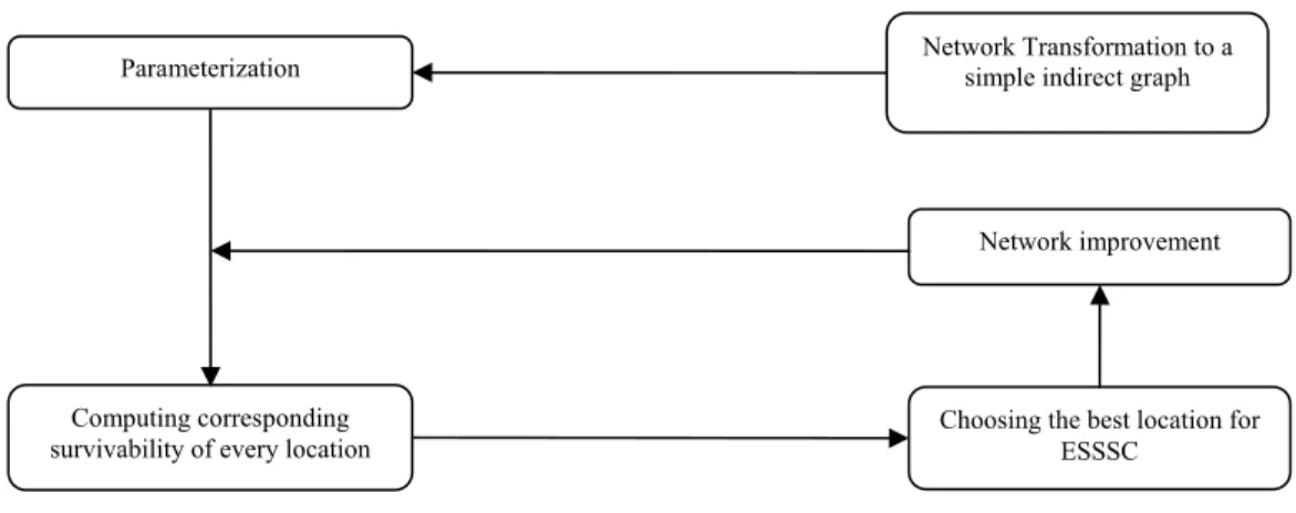
2. MODEL OVERVIEW
The proposed model is shown in Figure 1.
Figure 1 General Model
Suppose that a network of an imaginary region is provided. Due to the previous criteria, experts state some proposed locations appropriate for ESSSC. The stages are as follows.
Network Transformation: At first the network is transformed to a simple indirect corresponding graph G = (V, E), where V is a finite set of vertices and E is a set of edges, representing relations between pairs of vertices. The proposed locations for ESSSC are specified on the graph.
Network Transformation to a simple indirect graph Parameterization
Computing corresponding survivability of every location
Choosing the best location for ESSSC
Parameterization: As the region is mapped to vertices and edges of G, information such as survivability, time and cost of recovery of links must be assigned to edges.
Computing survivability: Once a weighted graph G is defined, the level of survivability of any part of the network can be computed. First of all, all edge-disjoint paths between proposed locations and all other nodes must be finding.
Having all edge-disjoint paths, the survivability of every edge, every edge-disjoint path and finally the total corresponding network of every proposed location are computed. Time and cost of recovery of links can be obtained in the same way.
Choosing the best location: By having survivability, time and cost of recovery for every proposed location, SAW (Simple Additive Weighting) method can be used to find the best location for the ESSSC and rank them. The following algorithm shows how the best location for ESSSCs can be found.
2.1. Algorithm
1. Transform the network to the corresponding simple and undirected graph.
2. Show the proposed locations for ESSSCs by capital letters and put them in a set named R. 3. Show the other nodes by small letters and put them in a set named N.
4. Select one of non-selected member of R, named K. if all of them are selected since now, go to step 10.
5. Find all edge-disjoint paths between K and other nodes, and put them in Edge-disjoint paths(K) = {Edge-disjoint paths (K, i) | i
N} 6. For each edge, (i, j), compute survivability of (i, j)For each edge-disjoint path (i…j), compute survivability (i…j)
Sur (i…j) = Mean Value {∑ Sur (a, b)} (a, b)
(i…j) 7. For each proposed location compute survivability of that locationSur (s) = Mean Value {Sur (s…j)} j
V-s8. Do the same for computing Time and cost of recovery of edges, edge-disjoint paths and network of every proposed location.
T(rec(i…j)) = Mean Value { ∑ T(rec (a,b)) } (a,b)
(i…j)C(rec(i…j)) = Mean Value { ∑ C(rec (a,b)) } (a,b)
(i…j)T (rec (s)) = Mean Value {T (rec (s…j))} j
V-s C (rec (s)) = Mean Value{C (rec (s…j))} j
V-s 9. Go to step 410. Develop the corresponding initial SAW (Simple Weighting Method) matrix, using values computed for every proposed location accused of the criteria.
11. Set the weighting vector, according to the importance of each criteria. 12. Apply SAW to the problem.
13. The output is the best solution for the problem.
Pseudo code Inputs:
N, original vertices set. R, proposed locations set. E, edges.
Sur, table of edges’survivabiliy Trec, table of edges’ recovery time Crec, table of edges’ recovery cost C, criteria vector
W, criteria weights vector Output:
Best location Method:
For each K
R do If R = Ø thenCall SAW (N, R, E, W); Else
Call ComputeNet (K); Procedure ComputeNet (K)
(1) for each v
N do(2) Edge-disjointpaths(K)← all of Edge-disjoint paths between K and v; (3) For each (i…j)
Edge-disjointpaths(K) do(4) Sur (i…j) ← Mean Value {∑ Surab} (a,b) (i…j) (5) Sur (K)← Mean Value{Sur (K…j)}
(6) T(rec (i…j)) ←Mean Value {∑ Trecab} (a,b) (i…j) (7) T(rec (K))← Mean Value{T(rec (K…j))}
(8) C(rec (i…j)) ←Mean Value {∑ Crecab} (a,b)
(i…j) (9) C(rec (K))← Mean Value{C(rec (K…j))}(10) R←R-K (11) Return; Procedure SAW
(1) for i = 1 to |R| do (2) SAWi1←Sur(Ki)
(3) SAWi2←T(rec (Ki))
(4) SAWi3←C(rec (Ki))
(5) for j = 1 do
(6) SAWij = SAWij/max(rij)
(7) for j = 2 or j = 3 do (8) SAWij = min(rij)/SAWij
(9) for i = 1 to |R| do (10) for j = 1 to 3 do (11) SAWij←SAWij*Wij (12) for i = 1 to |R| do (13) Value(Ki) =
3 1
j SAWij
(14) Find Max{Value(Ki)}
(15) Best Location←Ki
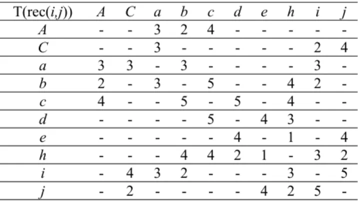
2.2. Numerical example
Suppose the graph shown in Figure 2 is obtained using the information of an original network. Proposed locations are shown with capital letters and other regions with small letters.
Figure 2 A Sample Graph So the inputs are as follows:
N :{ a, b, c, d, e, h, i, j} R: {A, C}
Sur, table of edges’ survivability
Table 1 Survivability of edges
j i h e d c b a C A Sur(i,j)
-5 3 4 -A 2 4 -3 -C -3 -4 -5 4 a -2 1 -2 -4 -3 b -3 -3 -2 -5 c -4 2 -3 -d 2 -1 -3 -e 3 2 -1 2 3 1 -h 3 -2 -2 3 4 -i -3 3 5 -2 -j
Trec, table of edges’ recovery time
Table 2 Time of recovery of failed edges j i h e d c b a C A T(rec(i,j))
-4 2 3 -A 4 2 -3 -C -3 -3 -3 3 a -2 4 -5 -3 -2 b -4 -5 -5 -4 c -3 4 -5 -d 4 -1 -4 -e 2 3 -1 2 4 4 -h 5 -3 -2 3 4 -i -5 2 4 -2 -j
Crec, table of edges’ recovery cost
a
b
h
e
i
j
A
c
d
C
Table 3 Cost of recovery of failed edges j i h e d c b a C A C(rec(i,j))
-3 2 4 -A 3 4 -2 -C -2 -2 -2 4 a -3 3 -4 -2 -2 b -3 -3 -4 -3 c -4 2 -3 -d 2 -3 -2 -e 3 3 -1 4 3 3 -h 2 -3 -3 2 3 -i -2 3 5 -4 -j
C: (Sur, Trec, Crec) W: (0.5, 0.25, 0.25) Method:
K = A
ComputeNet (K)
Sur (A) = Mean Value{8, 6, 7.3, 10.6, 10, 7, 7.3, 9.67} = 8.16 T (rec (A)) = Mean Value {T (rec (A…j))} j
V-s= Mean Value {7.3, 5.67, 8, 12, 11.67, 7.67, 7, 12} = 8.91 C (rec (A)) = Mean Value{C (rec (A…j))} j
V-s= Mean Value {6.34, 5, 7.3, 10, 9, 6.67, 6.67, 8.67} = 7.45 R←R-A
R← C K = C
ComputeNet (C)
Sur (C) = Mean Value {Sur (C …j)} j
V-s= Mean Value {6.67, 6.34, 9.34, 10, 9.34, 6.34, 5, 6.67} = 7.46
T (rec (C)) = Mean Value {T (rec (C …j))} j
V-s= Mean Value {7.34, 7, 12.34, 11.67, 11.34, 7.34, 5, 7.67} = 8.71 C (rec (C)) = Mean Value{C (rec (C …j))} j
V-s= Mean Value{6.34, 6.67, 11,67, 10.67, 9.67, 6.67, 4, 6.34} = 7075
R← Ø SAW
75
.
7
71
.
8
46
.
7
45
.
7
91
.
8
16
.
8
96
.
0
1
91
.
0
1
98
.
0
1
48
.
0
25
.
0
455
.
0
25
.
0
49
.
0
5
.
0
Sum1 = 1.24 Sum2 = 1.185
Max {Value (Ki)} ← 1.24
Best Location ← A
The solution is presented in more detail in Appendix. 2.3. Network Improvement
In the case where the total survivability of the network is low, the network potentially can be improved. So the edges with low levels of survivability must be obtained and after finding them, they are improved to do better and help the total network to have better services in disasters and unpredictable events.
3. CONCLUSIONS
In this paper a multi objective graph based model is presented in order to find the best one among several proposed locations for ESSSC. A simple additive weighting method helps the model in this way. This model can be usefully applied in defining the best location of other emergency and vital centers of communities which network survivability is an important factor for locating them. The proposed model can be developed by using directed corresponding graphs when is necessary. It can be also used different weights to test and derive a solution that is nearer to real situations.
REFERENCES
[1] Levitin, Gregory (2002), Maximizing survivability of acyclic transmission networks with multistate retransmitters and vulnerable nodes; Reliability Engineering and System Safety 77; 189–199.
[2] Korczak, Edward, Levitin, Gregory (2007), Survivability of systems under multiple factor impact; Reliability Engineering and System Safety 92; 269–274.
[3] Zeshung, Zhu, Ling, Sun (1998), A strategical model for analyzing survivability of environmental resource management system; IAPRS 32; 684.
[4] M. grotschel, C.L. Monma, M. Stoer (1995), Handbooks in OR & MS; Ch. 10, Vol. 7, Elsevier Science B.V..
[5] Charles A., Lauras M., Tomasini R. (2009), Learning from previous humanitarian operations, a business process reengineering approach; Proceeding of 6th International ISCRAM conference;
Sweden.
[6] Yuan Y., Dingwei W. (2009), Path selection model and algorithm for emergency logistics management; Computers and industrial engineering 56; 1081-1094.
[7] Cheu R., Huang Y., Huang B. (2008), Allocating emergency service vehicles to serve critical transportation infrastructures; Journal of Intelligent Transportation Systems; 38-49.
[8] Jia H., Ordenez F., Dessouki M. (2005), A modeling framework for facility location of medical services for large-scale emergencies; Create report, university of southern California.
[10] A.W. Krings, A. Azadmanesh (2005), A Graph Based Model for Survivability Applications; European Journal of Operational Research 164; 680–689.
Appendix
We provide a detailed solution for the numerical example 2.2: The inputs are as follows:
N :{a, b, c, d, e, h, i, j} R: {A, C}
Sur, table of edges’survivabiliy Trec, table of edges’ recovery time Crec, table of edges’ recovery cost C: (Sur, Trec, Crec)
W: (0.5, 0.25, 0.25) Method:
K = A
ComputeNet(K)
Edge-disjoint paths(K) = {Edge-disjoint paths (A,i) | i
N} Edge-disjoint paths (A, a) = Aa, Aba, AchiaEdge-disjoint paths (A, b) = Ab, Aab, Acb Edge-disjoint paths (A, c) = Ac, Abc, Aaihc Edge-disjoint paths (A, d) = Acd, Abhd, Aaijed Edge-disjoint paths (A, e) = Acde, Abhe, Aaije Edge-disjoint paths (A, h) = Aaih, Abh, Ach Edge-disjoint paths (A, i) = Aai, Abi, Achi Edge-disjoint paths (A, j) = Aaij, Abhj, Acdej
Sur(i…j) = Mean Value {∑ Surab} (a, b)
(i…j)= Mean Value {Sur(a,.) + … + Sur(., b)}
Sur(A…a) = Mean Value {Sur(Aa), Sur(Aba), Sur(Achia)} = Mean value {4, 7, 13} = 8 Sur(A…b) = Mean Value {Sur(Ab), Sur(Aab), Sur(Acb)} = Mean value {3, 8, 7} = 6 Sur(A…c) = Mean Value {Sur(Ac), Sur(Abc), Sur(Aaihc)} = Mean value {5, 5 , 12} = 7.3 Sur(A…d) = Mean Value {Sur(Acd), Sur(Abhd), Sur(Aaijed)} = Mean value {8, 6, 18} = 10.6 Sur(A…e) = Mean Value {Sur(Aaije), Sur(Acde), Sur(Abhe)} = Mean value {15, 10, 5} = 10 Sur(A…h) = Mean Value {Sur(Aaih), Sur(Abh), Sur(Ach)} = Mean value{9, 4, 8} = 7 Sur(A…i) = Mean Value {Sur(Aa), Sur(Abi), Sur(Achi)} = Mean value {7, 5, 10} = 7.3 Sur(A…j) = Mean Value {Sur(Aaij), Sur(Abhj), Sur(Acdej)} = Mean value {10, 7, 12} = 9. 67 Sur(s) = Mean Value {Sur(s…j)} j
V-sSur(A) = Mean Value {Sur(A…j)} j
V-sSur(A) = Mean Value{8, 6, 7.3, 10.6, 10, 7, 7.3, 9.67} = 8.16 T(rec(i…j) = Mean value {∑ T(rec(a,b)} (a,b)
( i…j)= Mean value {T(rec(a,.) + … + T(rec(., b)}
T(rec(A…a)) = Mean value {T(rec(Aa)), T(rec(Aba)), T(rec(Achia))} = Mean value {3, 5, 14} = 7.3 T(rec(A…b)) = Mean value {T(rec(Ab)), T(rec(Aab)), T(rec(Acb))} = Mean value {2, 6, 9} = 5.67 T(rec(A…c)) = Mean value {T(rec(Ac)), T(rec(Abc)), T(rec(Aaihc))} = Mean value {4, 7 13} = 8 T(rec(A…d)) = Mean value {T(rec(Acd)), T(rec(Abhd)), T(rec(Aaijed))} = Mean value {9, 8, 19} = 12 T(rec(A…e)) = Mean value {T(rec(Aaije)), T(rec(Acde)), T(rec(Abhe))} = Mean value {15, 13, 7} = 11.67 T(rec(A…h)) = Mean value {T(rec(Aaih)), T(rec(Abh)), T(rec(Ach))} = Mean value {9, 6, 8} = 7.67 T(rec(A…i)) = Mean value {T(rec(Aai)), T(rec(Abi)), T(rec(Achi))} = Mean value {6, 4, 11} = 7 T(rec(A…j)) = Mean value {T(rec(Aaij)), T(rec(Abhj)), T(rec(Acdej))} = Mean value {11, 8, 17} = 12 T(rec(s)) = Mean Value {T(rec(s…j))} j
V-sT(rec(A)) = Mean Value {T(rec(A…j))} j
V-s= Mean Value {7.3, 5.67, 8, 12, 11.67, 7.67, 7, 12} = 8.91 C(rec(i…j) = Mean value {∑ C(rec(a, b)} (a, b)
(i…j) = Mean value {C(rec(a,.) + … + C(rec(., b)}C(rec(A…a)) = Mean value {C(rec(Aa)), C(rec(Aba)), C(rec(Achia))} = Mean value {4, 4, 11} = 6.34 C(rec(A…b)) = Mean value {C(rec(Ab)), C(rec(Aab)), C(rec(Acb))} = Mean value {2, 6, 7} = 5 C(rec(A…c)) = Mean value {C(rec(Ac)), C(rec(Abc)), C(rec(Aaihc))} = Mean value {3, 6, 13} = 7.3 C(rec(A…d)) = Mean value {C(rec(Acd)), C(rec(Abhd)), C(rec(Aaijed))} = Mean value {6, 9, 15} = 10 C(rec(A…e)) = Mean value {C(rec(Aaije)), C(rec(Acde)), C(rec(Abhe))} = Mean value{13, 8, 6} = 9 C(rec(A…h)) = Mean value{C(rec(Aaih)), C(rec(Abh)), C(rec(Ach))} = Mean value {9, 5, 6} = 6.67 C(rec(A…i)) = Mean value {C(rec(Aai)), C(rec(Abi)), C(rec(Achi))} = Mean value{6, 5, 9} = 6.67 C(rec(A…j)) = Mean value {C(rec(Aaij)), C(rec(Abhj)), C(rec(Acdej))} = Mean value {8, 8, 10} = 8.67 C(rec(s)) = Mean Value{C(rec(s…j))} j
V-sC(rec(A)) = Mean Value{C(rec(A…j))} j
V-s= Mean Value {6.34, 5, 7.3, 10, 9, 6.67, 6.67, 8.67} = 7.45 R ← R-A
R ← C K = C
ComputeNet (C)
Edge-disjoint paths (K) = {Edge-disjoint paths (C, i) | i
N} Edge-disjoint paths (C, a) = Ca, Cia, CjhbaEdge-disjoint paths (C, b) = Cab, Cib, Cjhb Edge-disjoint paths (C, c) = Cabc, Cihc, Cjedc Edge-disjoint paths (C, d) = Cabcd, Cihd, Cjed Edge-disjoint paths (C, e) = Cabcde, Cihd, Cje
Edge-disjoint paths (C, h) = Cabh, Cih, Cjh Edge-disjoint paths (C, i) = Ci, Cai, Cji Edge-disjoint paths (C, j) = Cj, Cij, Cabhj
Sur(i…j) = Mean value {∑ Sur(a, b)} (a, b)
(i…j) = Mean value {Sur(a,.) + … + Sur(., b)}Sur (C …a) = Mean value {Sur(Ca), Sur(Cia), Sur(Cjhba)} = Mean value {3, 7, 10} = 6.76 Sur (C …b) = Mean value {Sur(Cab), Sur(Cib), Sur(Cjhb)} = Mean value {7, 6, 6} = 6.34 Sur (C …c) = Mean value {Sur(Cabc), Sur(Cihc), Sur(Cjedc)} = Mean value {9, 9, 10} = 9.34 Sur (C …d) = Mean value {Sur(Cabcd), Sur(Cihd), Sur(Cjed)} = Mean value {12, 8, 10} = 10 Sur (C …e) = Mean value {Sur(Cabcde), Sur(Cihe), Sur(Cje)} = Mean value {14, 7, 7} = 9.34 Sur (C …h) = Mean value {Sur(Cabh), Sur(Cih), Sur(Cjh)} = Mean value{8, 6, 5} = 6.34 Sur (C …i) = Mean value {Sur(Ci), Sur(Cai), Sur(Cji)} = Mean value{4, 6, 5} = 5 Sur (C …j) = Mean value {Sur(Cij), Sur(Cj), Sur(Cabhj)} = Mean value{2, 7, 11} = 6.67 Sur (s) = Mean Value {Sur (s…j)} j
V-sSur (C) = Mean Value {Sur (C …j)} j
V-s= Mean Value {6.67, 6.34, 9.34, 10, 9.34, 6.34, 5, 6.67} = 7.46
T(rec(i…j) = Mean value {∑ T(rec (a,b)} (a,b)
( i…j) = Mean value {T (rec (a,.) + … + T (rec (., b)}T(rec(C …a)) = Mean value {T(rec(Ca)), T(rec(Cia)), T(rec(Cjhba))} = Mean value {3, 5, 14} = 7.34 T(rec(C …b)) = Mean value {T(rec(Cab)), T(rec(Cib)), T(rec(Cjhb))} = Mean value {6, 4, 11} = 7 T(rec(C …c)) = Mean value {T(rec(Cabc)), T(rec(Cihc)), T(rec(Cjedc))} = Mean value {11, 9, 17} = 12.34 T(rec(C …d)) = Mean value {T(rec(Cabcd)), T(rec(Cihd)), T(rec(Cjed))} = Mean value {16, 7, 12} = 11.67 T(rec(C …e)) = Mean value {T(rec(Cabcde)), T(rec(Cihe)), T(rec(Cje))} = Mean value {20, 6, 8} = 11.34 T(rec(C …h)) = Mean value {T(rec(Cabh)), T(rec(Cih)), T(rec(Cjh))} = Mean value {10, 5, 7} = 7.34 T(rec(C …i)) = Mean value {T(rec(Ci)), T(rec(Cai)), T(rec(Cji))} = Mean value {2, 6, 7} = 5
T(rec(C …j)) = Mean value {T(rec(Cj)), T(rec(Cij)), T(rec(Cabhj))} = Mean value {4, 7, 12} = 7.67 T(rec(s)) = Mean Value {T(rec(s…j))} j
V-sT(rec(C)) = Mean Value {T(rec(C …j))} j
V-s= Mean Value {7.34, 7, 12.34, 11.67, 11.34, 7.34, 5, 7.67} = 8.71 C(rec(i…j) = Mean value {∑ C(rec(a, b)} (a, b)
(i…j)= Mean value {C(rec(a,.) + … + C(rec(., b)}
C(rec(C …a)) = Mean value {C(rec(Ca)), C(rec(Cia)), C(rec(Cjhba))} = Mean value {2, 6, 11} = 6.34 C(rec(C …b)) = Mean value {C(rec(Cab)), C(rec(Cib)), C(rec(Cjhb))} = Mean value {4, 7, 9} = 6.67 C(rec(C …c)) = Mean value {C(rec(Cabc)), C(rec(Cihc)), C(rec(Cjedc))} = Mean value {12, 10, 13} = 11.67 C(rec(C …d)) = Mean value {C(rec(Cabcd)), C(rec(Cihd)), C(rec(Cjed))} = Mean value {11, 11, 10} = 10.67
C(rec(C …e)) = Mean value {C(rec(Cabcde)), C(rec(Cihe)), C(rec(Cje))} = Mean value {13, 8, 8} = 9.67 C(rec(C …h)) = Mean value {C(rec(Cabh)), C(rec(Cih)), C(rec(Cjh))} = Mean value {7, 7, 6} = 6.67 C(rec(C …i)) = Mean value {C(rec(Ci)), C(rec(Cai)), C(rec(Cji))} = Mean value {3, 4, 5} = 4 C(rec(C …j)) = Mean value {C(rec(Cj)), C(rec(Cij)), C(rec(Cabhj))} = Mean value {3, 6, 10} = 6.34 C(rec(s)) = Mean Value{C(rec(s…j))} j
V-sC(rec(C)) = Mean Value{C(rec(C …j))} j
V-s= Mean Value{6.34, 6.67, 11,67, 10.67, 9.67, 6.67, 4, 6.34} = 7075
R←Ø SAW
75 . 7 71 . 8 46 . 7
45 . 7 91 . 8 16 . 8
96 . 0 1 91 . 0
1 98 . 0 1
48 . 0 25 . 0 455 . 0
25 . 0 49 . 0 5 . 0
Sum1 = 1.24 Sum2 = 1.185
Max {Value (Ki)} ←1.24