Ordinary Differential Equations

Ordinary Differential Equations

Dan B. Marghitu and S.C. Sinha

1

Introduction

Anordinary differential equationis a relation involving one or several

deriva-tives of a functiony(x) with respect tox. The relation may also be composed of constants, given functions of x, or y itself.

The equation

y0

(x) = ex_{, (1)}

where y0

=dy/dx, is of a first order ordinary differential equation, the equa-tion

y00

(x) + 2y(x) = 0, (2)

where y00

=d2_y/dx2 _{is of a second order ordinary differential equation, and}

the equation 2x2_y000 (x)y0 (x) + 3e−_xy00 (x) = (x2_{+ 1)y}2_{(x), (3)} where y000

=d3_y/dx3 _{is a third order ordinary differential equation.}

The orderof an ordinary differential equation the highest derivative of y

in the equation.

Definition [1]. The explicit solutionof a first-order differential equation

is a function

y=g(x), a < x < b, (4) defined and differentiable on (a, b), with the property that the equation be-comes an identity when y and y0

are replaced byg and g0

, respectively. The solution of a differential equationG(x, y) = 0 it is called theimplicit solution.

Example. The explicit solution of the first-order differential equation y0 (x) =x y(x), (5) is y(x) = c ex2_/2 , (6)

where c is an arbitrary constant. The differential equation (5) has many solutions. The function (6), with arbitrary c, represents the general solution

(the totality of all solutions of the equation). If we consider a definite value of c, for example c = 1, then the solution obtained y(x) = ex2_/2

is called a

particular solution.

2

First order differential equations

2.1

Separable equations

variable x appears only on the right hand side and the function y appears only on the left hand side in Eq. (8). Integrating both sides we obtain

Z

g(y)dy=Z f(x)dx+c. (9) Iff andg are continuous functions the general solution of Eq. (7) is obtained evaluating Eq. (9).

Example. Solve the equation

(y2_{+ 1)xdx+ (x+ 1)ydy= 0.}

The above equation can be rewritten in the form

x

x+ 1dx+

y

By integration we obtain

x−ln|1 +x|+₂1ln(1 +y2_{) =c, x+ 16= 0.}

With x= 0 andy= 0 we calculate c= 1₂ln 2 and 2x+ ln1 +y2

2 = ln(1 +x)2, x6=−1 .

Definition. A first-order differential equation together with an initial

condition is called an initial value problem. The initial condition is the

con-dition that at some point x = x0 the solution y(x) has a prescribed value

y(x0) = y0.

2.2

Equations reducible to separable form

y0

=gy x

, (10)

whereg is any given function of y/x(g(x) =f(y/x)), can be made separable equation by a simple change of variables. The change of variable is

y x =u.

The function y=u x and by differentiation we obtain

y0

=u+u0

x. (11)

Combining the equations (11) and (10), and taking into account thatg(y/x) =

g(u) we obtain

u+u0

x=g(u).

By separating the variables u and x, the previous equation takes the form

du g(u)−u =

dx x .

After integration and replacement ofubyy/xthe general solution of Eq. (10) is obtained.

Example. Solve the equation

dy dx =

2x+ 3y

3x+ 2y and 3x+ 2y6= 0.

With the change of function y=uxwe obtain

u0 x+u= 2 + 3_{3 + 2}u_u or u0 x= 2_{3 + 2}−2u_u2 and 1 2 3 + 2u 1−u2du= dx x . Integrating Z dx x = 1 2 Z 3 + 2u 1−u2du or ln|x|=−1 2ln|u2−1| − 3 4ln 1−u 1 +u + ln|c|. We obtainx4_(u2₋₁₎21−u 1 +u 3

=c. Replacingubyy/x, the general integral will be

(x2_−y2₎2_(x−y)3 _=c(x+y)3_.

2.3

Exact differential equations

is exact if the left hand side is an exact differential

d u(x, y) = ∂u

∂xdx+ ∂u

∂ydy. (13)

Equation (12) can be rewritten as

d u= 0.

and by integration the general solution is

u(x, y) = c. (14)

If there is a functionu(x, y) with the properties (a)∂u

∂x =M, (b) ∂u

∂y =N, (15)

then M(x, y)dx+N(x, y)dy = 0 is an exact differential equation.

The necessary and sufficient condition forMdx+Ndybe an exact differ-ential [1] is

∂M ∂y =

∂N

∂x. (16)

To find u(x, y) we have the following steps [1].

From Eq. (15.a) if we consider y to be a constant we obtain

u=Z Mdx+k(y), (17) where and k(y) is the “constant” of integration.

k(y) is determined from Eq. (17) deriving ∂u/∂y. From Eq. (15.b) we getdk/dy.

Example. Solve the equation

− x

2x−yy

0

+ ln(2x−y) + 2x

2x−y = 0 2x−y >0.

Writing the equation in the form Eq. (12), we get

− x 2x−ydy+ " ln(2x−y) + 2x 2x−y # dx= 0 (18)

Equation (18) is exact. ConsiderM = ln(2x−y)+ 2x

2x−y, andN =− x

2x−y.

Then, by differentiation we obtain

∂M ∂y = −1 2x−y + 2x (2x−y)2, ∂N ∂x = −1 2x−y + 2x (2x−y)2.

From Eq. (15.b) we have N = ∂u_∂y and by integration

u=xln(2x−y) +k(x).

To determine k(x) we differentiate u and apply Eq. (15.a)

∂u ∂x = ln(2x−y) + 2x 2x−y + dk dx =M.

By simple algebraic manipulations, we find that dk

dx = 0 and, consequently, k(x) =c, wherec is an arbitrary constant. We obtain the final form

xln(2x−y) = c.

2.4

Linear differential equations

y0

+f(x)y=r(x), (19)

which is linear in y and y0

(f and r may be any given functions of x). Ifr(x) = 0, ∀x (for allx) the equation is homogeneous. For r(x)6= 0 the

equation is said to be nonhomogeneous.

Assuming thatf(x) and r(x) are continuous for x∈I, we need to find a general formula for Eq. (19).

Case I. homogeneous equation

For the equation

y0

separating variables we have

dy

y =−f(x)dx or ln|y|=−

Z

f(x)dx+c∗_,

and the solution is

y(x) =ce−Rf(x)dx _(c=±ec∗

wheny <0 or y >0). (21)

Case II. nonhomogeneous equation

Multiplying Eq. (19) by F(x) =eh(x) _{where h(x) =} Z _f(x)dx. we find eh_(y0 +fy) = eh_r. Since h0 =f, we obtain d dx(yeh) =ehr.

Integrating the above relation we have

yeh ₌Z _eh_rdx+c.

The general solution of Eq. (19) in the form of an integral may be written

y(x) =e−_hZ _{ehrdx+c, h=}Z _{f(x)dx. (22)}

Example. Solve the differential equation

xy0

+ (1−x)y=xex_.

We can rewrite the equation in the form

y0

+1_x −1y=ex_.

Comparing the previous equation to Eq. (22) we can identify

no constant being added in the integration. Thus, the solution will be y = e−_logx+xZ _elogx−_{xex dx+c} = e_xxZ _ex_xex _dx+c, or y=exx 2 + c x ,

where cis an arbitrary constant.

2.5

Variation of parameters

Another way of finding the general solution of linear differential equation

y0

+f(x)y=r(x). (23)

is the method of variation of parameters.

The solution corresponding to a homogeneous equation (r(x) = 0) is

v(x) =e−R_{f(x)dx. (24)}

With Eq. (24) we try to determine a function u(x) such that

y(x) =u(x)v(x), (25) is the general solution of Eq. (23). This approach is called the method of variation of parameters [1].

Equations (25) and Eq. (23) can be combined into

u0 v+u(v0 +fv) = r, or u0 v =r, sincev0 +fv = 0. We findu0 = r v and by integration u=Z _vrdx+c.

We obtain the general solution

y =uv =vZ r_vdx+c, (26) which is identical with Eq. (22) of the previous section.

3

Second order differential equation

3.1

Homogeneous linear equations

A second-order differential equation which can be written as

y00

+f(x)y0

+g(x)y=r(x) (27)

is said to be linear. It is said to be nonlinear if it cannot be written in the

form of Eq. (27). The functions f and g are called the coefficients of the

equation (27).

Ifr(x)6= 0, then Eq. (27) is said to be nonhomogeneous. Otherwise, it is

said to be homogeneous and takes the form

y00

+f(x)y0

+g(x)y= 0. (28)

It is called a solutionof a differential equation of the second order on an

interval J a function y =φ(x) which is defined and two times differentiable on J. Moreover, the equation becomes an identity if φ and its derivative replace the unknown function y and its derivatives, respectively. For the case of homogeneous equations, the following theorem states that solutions of Eq. (28) can be obtained from known solutions by multiplication by constants and by addition.

Fundamental Theorem [1]. If a solution of the homogeneous linear

differential equation (28) on the interval J is multiplied by any constant, the resulting function is also a solution of Eq. (28) on J. The sum of two solutions of Eq. (28) on J is also a solution of Eq. (28) on that interval.

Proof. We assume that φ(x) obeys the conditions to be a solution of

Eq. (28) on J. If we replace y bycφ(x) is into Eq. (28), we obtain (cφ)00

+f(cφ)0

+gcφ=c[φ00 +fφ0

+gφ].

Since φ is a solution of Eq. (28), thenφ00 +fφ0

+gφ = 0 and we find thatcφ

is also a solution of Eq. (28). The second part of the theorem can be proved in the same way.

Example. The functions y₁ = φ₁ = x and y₂ = φ₂ = x2, x ∈ R − {0}

(J ≡ R − {0}), are two solutions of the equation

x2_y00

−2xy0

+ 2y= 0.

3.2

Homogeneous equations with constant coefficients

y00 +ay0

+by= 0, (29)

where a, b ∈ R are constants, and x ∈ R. The solution of the first-order homogeneous linear equation with constant coefficients

y0 +ky = 0, is an exponential function, y=C e−_kx. We assume that y=eλx_{, (30)}

may be a solution of Eq. (29) if λ is properly chosen. Substituting Eq. (30) and its derivatives

y0

=λeλx _{and y}00

=λ2_eλx_,

into Eq. (29), we obtain

(λ2_+aλ+b)eλx_{= 0.}

So Eq. (30) is a solution of Eq. (29), if λ is a solution of the equation

λ2_{+aλ+b = 0. (31)}

Eq. (31) is called the characteristic equationof Eq. (29). Its roots are

λ1 = 1₂(−a+ √ a2_{−4b), λ2 =} 1 2(−a− √ a2_{−4b). (32)}

From derivation it follows that the functions

y1 =eλ1x and y2 =eλ2x, (33)

are solutions of Eq. (29). This result can be verified by substituting Eq. (33) into Eq. (29).

Elementary algebra states that, since a and b are real, the characteristic equation may have

Case I two distinct real roots,

Case II two complex conjugate roots, or

Case III a real double root.

Example 1. Solve the equation

2y00 −5y0

+ 2y= 0.

The characteristic equation of the given differential equation will be 2λ2_{−5λ+ 2 = 0}

so that

λ1 = 1₂, λ2 = 2.

Then the general solution is

y=c1ex/2+c2e2x.

Example 2. The equation

y00 + 2y0

+ 5y= 0 has the characteristic equation

λ2_{+ 2λ+ 5 = 0}

from which

λ1,2 =−1±2i.

The general solution will be

y =e−x_(c

1cos 2x+c2sin 2x).

Example 3. The equation

y00 −2y0

+ 1 = 0 has the characteristic equation

(λ−1)2 _{= 0}

which gives

λ1,2 = 1.

We obtain the general solution

3.3

General solution. Fundamental system

Definition. The general solution of a second order differential equation

is a solution which contains two arbitrary independent constants, i.e. the solution cannot be reduced to a form containing only one arbitrary constant or none. Aparticular solutionis a solution obtained from the general solution

assigning specific values to the arbitrary constants. We consider the general homogeneous linear equation

y00

+f(x)y0

+g(x)y= 0, (34)

and two solutions y1(x) andy2(x) of this equation. The Fundamental

Theo-rem states that

y(x) = c1y1(x) +c2y2(x), (35)

is a general solution of Eq. (34), where c1 andc2 are two arbitrary constants.

Two functionsy1(x) and y2(x) arelinearly dependenton an open interval

I where both functions are defined, if they are proportional on I

(a)y1 =m y2 or (b)y2 =n y1, (36)

for all x ∈ I, where m and n are numbers. If the functions are not propor-tional, they are linearly independentonI.

If at least one of the functionsy1 andy2 is identically zero on I, then the

functions are linearly dependent on I. In any other case the functions are linearly dependent on I if and only if the quotient y1/y2 is constant on I.

Hence, if y1/y2 depends on x on I, then y1 and y2 are linearly independent

on I [1].

Example 1. The functions

y1 = 9x and y2 = 3x

are linearly dependent, because the quotient y1/y2 = 3 = const while the

functions

y1 =x2+x and y2 =x

are linearly independent because y1/y2 =x+ 16= const.

Two linearly independent solutions of Eq. (34) on I constitute a funda-mental system or a basis of solutions on I.

Theorem[1]. The solution

y(x) =c1y1(x) +c2y2(x) (c1, c2arbitrary)

is a general solution of the differential equation Eq. (34) on an interval I of the x-axis if and only if the functions y₁ and y₂ constitute a fundamental system of solutions of Eq. (34) onI. y₁ andy₂ constitute such a fundamental system if and only if their quotient y₁/y₂ is not constant on I but depends on x.

Example 2. The equation

y00 −2y0

−15y= 0 has the solutions

y1 =e5x and y2 =e−3x.

These solutions constitute a fundamental system because the ratio y1/y2 is

not constant. The general solution is

y=c1y1+c2y2 =c1e5x+c2e−3x.

3.4

Complex roots of the characteristic equation.

Ini-tial value problem

The solutions of the homogeneous linear equation with constant coefficients

y00 +ay0

+by = 0 (a, b real) (37)

are

y1 =eλ1x and y2 =eλ2x, (38)

where λ1 and λ2 are the roots of the corresponding characteristic equation

λ2_{+aλ+b = 0. (39)}

In the case of λ1 6=λ2, the quotient y1/y2 is not constant, and the solutions

constitute a fundamental system for all x. The general solution is

The solutions of the Eq. (38) are real if the distinct roots of the corre-sponding characteristic equation are real (Case I). If λ1 and λ2 are complex

conjugate roots of the form (Case II)

λ1 =p+i q, λ2 =p−i q,

then the solutions Eq. (38) are complex

y1 =e(p+i q)x, y2 =e(p−i q)x.

The real solutions can be derived from the complex solutions by applying the Euler formulas

eiθ _{= cosθ+isinθ, e}−iθ _{= cosθ−isinθ,}

for θ =qx. The first solution becomes

y1 =e(p+iq)x =epxeiqx=epx(cosqx+isinqx),

while the second one is

y2 =e(p−iq)x =epxe−iqx=epx(cosqx−isinqx).

From Fundamental Theorem we can conclude that they are solutions of the differential equation Eq. (37). The corresponding general solution is

y(x) =epx_{(Acosqx+Bsinqx) (41)}

where A and B are arbitrary constants.

Example 1. Let us consider the second order differential equation with

constant coefficients

y00 −4y0

+ 5y= 0 The corresponding characteristic equation is

λ2_{−4λ+ 5 = 0,}

with the roots

For this example p= 2, q= 1, and from Eq. (41) the answer is

y=e2x_{(Acosx+Bsinx).}

Let us consider the values of the solutiony(x) and its derivative y0 (x) at an initial point x=x0

y(x0) = K, y0(x0) =L, (42)

The conditions Eq. (42) and the equation Eq. (37) constitute an initial value problem. To solve such a problem we must find a particular solution of

Eq. (37) satisfying Eq. (42). Such a problem has a unique solution.

Example 2. Let us consider the initial value problem

y00 −4y0

+ 5y = 0, y(0) = 2, y0

(0) = 0.

A fundamental system of solutions is

e2x_{cosx and e}2x_sinx,

and the corresponding general solution is

y(x) = e2x_{(Acosx+Bsinx),}

with the initial condition y(0) =A. The derivative

y0

=e2x_{[(2A+B) cosx+ (2B−A) sinx)],}

has the initial value y0

(0) = 2A+B. Solving the initial conditions system,

y(0) =A= 2, y0

(0) = 2A+B = 0.

we get A = 4,B =−1, and the general solution of the differential equation is

3.5

Double root of the characteristic equation

Now we consider the case when the characteristic equation associated to a homogeneous linear differential equation with constant coefficients has a double root (critical case). If the differential equation takes the general form

y00 +ay0

+by= 0, (44)

then the characteristic equation will be

λ2_{+aλ+b = 0. (45)}

A double root appears if an only if the discriminant of Eq. (45) is zero, that is

a2_{−4b= 0, and, then, b =} 1

4a2.

The double root of the characteristic equation is λ =−a/2. Then, the first solution of the differential equation is

y1 =eax/2. (46)

To find another solutiony2(x) the method of variation of parameters may

be applied. The second solution takes the form

y2(x) = u(x)y1(x) where y1(x) =e−ax/2.

Substituting y2 in the differential equation with b=a2/4 we obtain

u(y00 1 +ay 0 1+1₄a2y1) +u 0 (2y0 1+ay1) +u 00 y1 = 0.

The expression in the first parentheses is zero because y1 is a solution. The

second parentheses is also zero because 2y0 1 = 2 −a 2 e−_{ax/2 =−ay} 1.

The equation reduces to u00

y1 = 0, and a solution is u = x. Consequently,

the second solution is

y2(x) =xeλx

We can observe that the solutions y1 and y2 are linearly independent. This

case can be summarized by the following theorem

Theorem (Double root) [1]. In the case of a double root of Eq. (45)

the functions (46) and (47) are solutions of Eq. (44). They constitute a fundamental system. The corresponding general solution is

y= (c1+c2x)eλx

λ=−a₂. (48)

Example. Solve the following differential equation

y00 −4y0

+ 4y=O.

The double root of the characteristic equation is λ= −4. Then, the funda-mental system of solutions is

e2x _{and xe}2x

and the corresponding general solution is

y = (c1+c2x)e2x.

All three cases are summarized in the following table:

Case Roots of Eq. (45) Fundamental General solution of Eq. (44)

system of Eq. (44)

I Distinct real eλ1x, eλ2x y=c

1eλ1x+c

2eλ2x

λ1, λ2

II Complex conjugate epx_{cosqx y=e}px_{(Acosqx+Bsinqx)}

λ1 =p+iq, epxsinqx

λ2 =p−iq

III Real double root eλx_{, xe}λx _{y= (c}

1+c2x)eλx

λ =−a/2

3.6

Series solutions

We consider the general homogeneous linear second-order equation

withP(x)6= 0 in the intervalα < x < β. We want to determine a polynomial solution y(x) of Eq. (49).

Definition. A functions f(x) can be expanded in power series so that

f(x) =a0+a1(x−x0) +a2(x−x0)2+. . .=

∞ X

n=0an(x−x0)

n_{. (50)}

Such functions are said to be analytic at x=x₀ and the series (50) is called

the Taylor series of f about x = x0. The coefficients an can be computed

with the formula an =f(n)(x0)/ n! where f(n)(x) = dnf(x)/dxn.

We consider the functionsP(x),Q(x), and R(x) as power series aboutx0

P(x) =p0+p1(x−x0) +. . . , Q(x) =q0+q1(x−x0) +. . . ,

R(x) = r0+r1(x−x0) +. . .

and y(x) = a0+a1(x−x0) +. . ..

Theorem[2]. Let the functions Q(x)/P(x) andR(x)/P(x) have

conver-gent Taylor series expansions about x = x₀ for |x−x₀| < ρ. Then, every solution y(x) of the differential equation

P(x)d_dx2y₂ +Q(x)dy_dx +R(x)y= 0 (51)

is analytic at x = x₀, and the radius of convergence of its Taylor series expansion about x=x₀ is at least ρ. The coefficients a₂, a₃, . . . in the Taylor series expansion

y(x) = a0+a1(x−x0) +a2(x−x0)2+. . . (52)

are determined by plugging the series (52) into the differential equation (51) and setting the sum of the coefficients of the like powers ofxin this expression equal to zero.

Example. Solve the equation

x2d2y

dx2 + (x2+x)

dy

dx −y= 0.

Assuming a solution of the form

y=

∞ X

k=0akx

we obtain dy dx = ∞ X k=0 kakxk−1, d 2_y dx2 = ∞ X k=0 k(k−1)akxk−2, and hence ∞ X k=0 k(k−1)akxk+ ∞ X k=0 kakxk+1+ ∞ X k=0 kakxk− ∞ X k=0 akxk.

The first, third, and fourth summations may be combined to give

∞ X k=0 [k(k−1) +k−1]akxk = ∞ X k=0 (k2_−1)a kxk,

and hence there follows

∞ X k=0(k 2 _−1)a kxk+ ∞ X k=0kakx k+1_.

In order to combine these sums, we replace k bynin the first and (k+ 1) by

n in the second, to obtain

∞ X n=0 (n2_−1)a nxn+ ∞ X n=1 (n−1)an−₁xn.

Since the ranges of summation differ, the term corresponding to n= 0 must be extracted from the first sum, after which the remainder of the first sum can be combined with the second. In this way we find

−a0 + ∞ X n=1 [(n2_−1)a n+ (n−1)an−₁]xn.

In order that the previous relation may vanish identically, the constant term, as well as the coefficients of the successive powers of x, must vanish indepen-dently, giving the condition

a0 = 0

and the recurrence formula

The recurrence formula is automatically satisfied when n= 1. When n≥2, it becomes

an=−_nan_{+ 1}−1 (n = 2,3,4. . .).

Hence, we obtain

a2 =−a₃1, a3 =−a₄2 = ₃a_·1₄, a4 =−a₅3 =−_3·a₄1_·5, . . . .

Thus, in this case a0 = 0, a1 is arbitrary, and all succeeding coefficients are

determined in terms of a1. The solution becomes

y=a1 x−x 2 3 + x3 3·4 − x4 3·4·5 +. . . ! .

If this solution is put in the form

y = 2_xa1 x_2!2 − x_3!3 +x_4!4 − x_5!5 +. . . ! = 2a1 x " x−1 + 1− x 1!+ x2 2! − x3 3! + x4 4! −. . . !# ,

the series in parentheses in the final form is recognized as the expansion of

e−x_{, and, writing 2a}

1 = c, the solution obtained may be put in the closed

from

y =c e−x−_x1 +x

!

.

In this case only one solution was obtained. This fact indicates that any linearly independent solutions cannot be expanded in power series nearx= 0. That is, it is not regular at x= 0.

3.7

Regular singular points

x2d2y

dx2 +αx

dy

which can be rewritten in the form d2_y dx2 + α x dy dx + β x2y= 0. (54)

A generalization of Eq. (54) is the equation

d2_y

dx2 +p(x)

dy

dx +q(x)y= 0 (55)

where p(x) andq(x) can be expanded in series of the form

p(x) = p_x0 +p1+p2x+p3x2+. . .

q(x) = _xq0₂ +q_x1 +q2+q3x+q4x2. . .

(56)

Definition [2]. Equation (55) is said to have a regular singular point at

x= 0 if p(x) andq(x) have series expansions of the form (56). Equivalently,

x= 0 is a regular singular point of Eq. (55) if the functionsx p(x) andx2_q(x)

are analytic at x= 0. Equation (55) is said to have a regular singular point at x = x0 if the functions (x−x0)p(x) and (x−x0)2q(x) are analytic at

x=x0. A singular point of Eq. (55) which is not regular is called irregular.

Example. Classify the singular points of Bessel’s equation of order ν

x2d2y

dx2 +x

dy

dx+ (x2−ν2)y= 0, (57)

where ν is a constant [1].

For x = 0 we have P(x) = x2 _{= 0. Hence, x = 0 is the only singular}

point of Eq. (57). Dividing both sides of Eq. (57) by x2 _gives

d2_y dx2 + 1 x dy dx + 1− ν2 x2 ! y= 0. The functions x p(x) = 1 and x2_{q(x) = x}2_−ν2

are both analytic at x= 0. Hence Bessel’s equation of order ν has a regular singular point at x= 0.

3.8

Nonhomogeneous linear equations

Let us consider a second-order linear nonhomogeneous equation

y00

+f(x)y0

+g(x)y=r(x). (58)

A general solution y(x) of Eq. (58) can be obtained from a general solu-tion yh(x) of the corresponding homogeneous equation

y00

+f(x)y0

+g(x)y= 0,

by adding toyh(x) any particular solution ˜yof Eq. (58) involving no arbitrary

constant [1]

y(x) =yh(x) + ˜y(x). (59)

To show thaty(x) is a solution of the nonhomogeneous differential equa-tion we substitute Eq. (59) into Eq. (58). Then the left-hand side of Eq. (58) becomes (yh+ ˜y) 00 +f(yh+ ˜y) 0 +g(yh+ ˜y). or (y00 h+fy 0 h+gyh) + ˜y 00 +fy˜0 +gy.˜

The expression in the parentheses is zero because yh is a solution of Eq.

(59). The sum of the other terms is equal to r(x) because ˜y satisfies Eq. (58). Hence y(x) is a general solution of the Eq. (58).

Theorem [1]. Suppose that f(x), g(x), and r(x) in Eq. (58) are

con-tinuous functions on an open interval I. Let Y(x) be any solution of Eq. (58) onI containing no arbitrary constants. ThenY(x)is obtained from Eq. (59) by assigning suitable values to the two arbitrary constants contained in the general solution y_h(x) of Eq. (59). In Eq. (59), the functiony˜(x) is any solution of Eq. (58) on I containing no arbitrary constants.

Proof. Let set Y −y˜=y∗. Then

y∗00 +fy∗0 +gy∗ _{= (Y}00 +fY0 +gY)−(˜y00 +fy˜0 +gy˜) =r−r= 0,

that is,y∗_{is a solution of Eq. (59) which does not contain arbitrary constants.}

It can be obtained from yh by assigning suitable values to the arbitrary

Theorem [1]. A general solution y(x) of the linear nonhomogeneous differential equation Eq. (58) is the sum of a general solution y_h(x) of the corresponding homogeneous equation Eq. (59) and an arbitrary particular solution y_p(x) of Eq. (58):

y(x) =yh(x) +yp(x) (60)

.

Example. Solve the equation

y00

+y= secx.

The homogeneous equationy00

+y= 0 has the characteristic equationλ2_{+ 1 = 0}

with roots λ1 =i and λ2 =−i, so, the general solution of the homogeneous

equation is

y=c1cosx+c2sinx.

Using the method of variation of parameter we have the following system of equations c0 1cosx+c 0 2sinx= 0, −c0 1sinx+c 0 2cosx= secx,

with the solution

c0 1 =−tanx, c 0 2 = 1. Thus by integrating, c1 =−ln secx+A1, c2 =x+A2,

and the general solution is of the nonhomogeneous equation is

y=A1cosx+A2sinx−cosxln secx+xsinx.

3.9

The method of variation of parameters

This method can be applied to solve the nonhomogeneous equation of the form

d2_y

dx2 +p(x)

dy

once the solutions of the homogeneous equation

d2_y

dx2 +p(x)

dy

dx +q(x)y= 0 (62)

are known. Let y1(x) and y2(x) be two linearly independent solutions of the

homogeneous equation (62). We will try to find a particular solution ψ(x) of the nonhomogeneous Eq. (61) of the form [2]

ψ(x) =u1(x)y1(x) +u2(x)y2(x). (63)

The differential equation (61) imposes only one condition on the two unknown functions u1(x) andu2(x). We may impose an additional condition on u1(x)

and u2(x) such that the left hand side of the nonomogeneous equation be as

simple as possible. Computing

d dxψ(x) = d dx[u1y1+u2y2] = [u1y 0 1 +u2y 0 2] + [u 0 1y1+u 0 2y2]

we see that d2_ψ/dx2 _{will contain no second-order derivatives ofu}

1 and u2 if y1(x)u 0 1(x) +y2(x)u 0 2(x) = 0. (64)

Imposing the condition (64) on the functions u1(x) and u2(x) the left hand

side of the Eq. (61) becomes [u1y 0 1+u2y 0 2] 0 +p(x)[u1y 0 1+u2y 0 2] +q(x)[u1y1+u2y2] = u0 1y 0 1+u 0 2y20+u1[y 00 1 +p(x)y 0 1+q(x)y1] +u2[y 00 2 +p(x)y 0 2+q(x)y2] = u0 1y 0 1+u 0 2y 0 2.

Ifu1(x) and u2(x) satisfy the two equations

y1(x)u 0 1+y2(x)u 0 2(x) = 0 y0 1(x)u 0 1(x) +y 0 2(x)u 0 2(x) = g(x),

then ψ(x) =u1y1+u2y2 is a solution of the nonhomogeneous equation (61).

We solve the above system of equations as follows h y1(x)y 0 2(x)−y 0 1(x)y2(x) i u0 1(x) =−g(x)y2(x) h y1(x)y 0 2(x)−y 0 1(x)y2(x) i u0 2(x) =g(x)y1(x).

The function u0 1(x) and u 0 2(x) are u0 1(x) =−_Wg(_[yx)y2(x) 1, y2](x) and u 0 2(x) = _Wg(_[yx)y1(x) 1, y2](x), (65)

where W[y1, y2](x) is the Wronskian of the solutions

W[y1, y2](x) = y1 y2 y0 1 y 0 2 .

Integrating the right-hand sides of Eqs. (65) we obtain u1(x) and u2(x).

Example.

(a) Find a particular solution ψ(x) of the equation

d2_y

dx2 + 4y= 8 sinx (66)

(b) Find the solution y(x) of Eq. (66) which satisfies the initial conditions

y(0) = 1, y0

(0) = 1.

(a) The functions y1(x) = cos 2x and y2(x) = sin 2x are two linearly

inde-pendent solutions of the homogeneous equation y00

+ 4y= 0 with

W[y1, y2](x) = y1y

0

2−y

0

1y2 = (cosx) cosx−(−sinx) sinx= 1.

Thus, from Eqs. (65),

u0

1(x) = −8 sin2x and u

0

2(x) = 8 sinxcosx. (67)

Integrating the first equation of (67) gives

u1(x) = −8

Z

sin2_{x dx=−4}Z _{(1−cos 2x)dx}

= −4Z dx+ 4Z cos 2x dx

= −4x+ 2 sin 2x.

while integrating the second equation of (67) gives

u2(x) =

Z

Consequently,

ψ(x) = cosx[−4x+ 2 sin 2x] + sinx(−2 cos 2x) is a particular solution of Eq. (66).

(b)

y(x) =c1cosx+c2sinx+ cosx(−4x+ 2 sin 2x)−2 sinxcos 2x

for some choice of constants c1, c2. The constants c1 and c2 are determined

from the initial conditions

1 = y(0) =c1 and 1 =y

0

(0) =c2−2.

Hence, c1 = 1, c2 = 3 and

y(x) = cosx+ 3 sinx+ cosx(−4x+ 2 sin 2x)−2 sinxcos 2x.

4

Differential equations of arbitrary order

4.1

Homogeneous linear equations

A linear differential equation of nth order can be written in the following

general form

y(n)_+f

n−1(x)y(n−1)+. . .+f1(x)y

0

+f0(x)y =r(x) (68)

where the functionron the right-hand side and the coefficientf0, f1, . . . , fn−1

are any given functions of x, and y(n) _{is thenth derivative of y.}

Eq. (68) is said to be homogeneous if r(x) = 0. Then, Eq. (68) becomes

y(n)_+f

n−₁(x)y(n−1)+. . .+f₁(x)y

0

+f0(x)y= 0. (69)

If r(x)6= 0, Eq. (68) is said to benonhomogeneous.

A function y = φ(x)is called a solution of a differential equation of nth

order on an intervalI if φ(x) is defined andntimes differentiable on I and is such that the equation becomes an identity when we replace the unspecified

function y and its derivatives in the equation by φ and its corresponding derivatives [1].

Existence and uniqueness theorem [1], [3]. If f₀(x), . . . , f_n−1(x) in

Eq. (69) are continuous functions on an open interval I, then the initial value problem consisting of the equation Eq. (69) and the n initial conditions

y(x0) = K1, y

0

(x0) = K2, . . . , y(n−1)(x0) =Kn,

has a unique solutiony(x)onI; herex₀is any fixed point inI, andK₁, . . . , K_n are given numbers .

A set of functions,y1(x), . . . , yn(x) arelinearly dependenton some interval

I where they are defined, if one of them can be represented onI as a “linear combination” of the othern−1 functions. Otherwise the functions arelinearly independent on I.

A fundamental system or a basis of solutions of the linear homogeneous

equation Eq. (69) is a set ofnlinearly independent solutionsy1(x), . . . , yn(x)

of that equation.

Ify1, . . . , yn is such a fundamental system, then

y(x) =c1y1(x) +. . .+cnyn(x) (c1, . . . , cnarbitrary) (70)

is a general solution of Eq. (69) on I. The test for linear dependence and independence of solutions can be generalized tonth order equations as follows

Theorem[1]. Suppose that the coefficientsf₀(x), . . . , f_n−1(x)of Eq. (69)

are continuous on an open intervalI. Then nsolutionsy₁, . . . , y_nof Eq. (69) on I are linearly dependent on I if and only if their Wronskian

W(y1, . . . , yn) = y1 y2 . . . yn y0 1 y 0 2 . . . y 0 n .. . ... . . . ... y(n−1) 1 y(2n−1) . . . yn(n−1) (71)

is zero for some x=x₀ in I. (If W = 0 at x=x₀, then W ≡0 on I).

Theorem [1]. Let Eq. (70) be a general solution of Eq. (69) on an

open interval I where f₀(x), . . . , f_n−1(x) are continuous, and letY(x) be any

solution of Eq. (69) on I involving no arbitrary constants. Then Y(x) is obtained from Eq. (70) by assigning suitable values to the arbitrary constants

Example. The equation

y000 −2y00

−y0

+ 2y= 0. (72)

has the solutions y1 =ex, y2 =e2x, and y3 =e3x.

The Wronskian is W(ex_{, e}2x_{, e}3x_{) =} ex _e2x _e3x ex _2e2x _3e3x ex _4e2x _9e3x = 2e6x_{6= 0,}

which shows that the functions constitute a fundamental system of solutions of Eq. (72). The corresponding general solution is

y=c1ex+c2e2x+c3e3x.

4.2

Homogeneous linear equations with constant

coef-ficients

A linear homogeneous equation of order n with constant coefficients

y(n)_+a

n−₁y(n−1)+. . .+a₁y

0

+a0y= 0, (73)

has the correspondent characteristic equation

λn_+a

n−₁λn−1+. . .+a₁λ+a₀ = 0. (74)

If this equation has n distinct roots λ1, . . . , λn, then the n solutions

y1 =eλ1x, . . . , yn =eλnx (75)

constitute a fundamental system for all x, and the corresponding general solution of Eq. (73) is

y=c1eλ1x+. . .+cneλnx. (76)

Ifλ is a root of order m, then

eλx_{, xe}λx_{, . . . , x}m−1_eλx ₍₇₇₎

Example. Consider the differential equation

y000 + 3y00

−4y0

−12y= 0.

The characteristic equation

λ3_{+ 3λ}2_{−4λ+ 12 = 0}

has the solutions λ1 = −2, λ2 = 2, and λ3 = −3, and the corresponding

general solution Eq. (76) is

y=c1e−2x+c2e2x+c3e−3x.

4.3

Linear differential equations in state space form

an(t)d n_y

dtn +an−1(t)d

n−_1y

dtn−₁ +. . .+a0y= 0,

can be transformed into a system of n first order equations. With the notations

x1(t) =y, x2(t) =dy/dt, . . . xn(t) =dn−1y/dtn−1,

we obtain the system

dx1 dt =x2, dx2 dt =x3, . . . , dxn−₁ dt =xn, and dxn dt =− an−₁(t)x_n+a_n−₂(t)x_n−₁+. . .+a₀x₁ an(t) .

A system of n first-order linear equations has the general form

dx1 dt =a11(t)x1+. . .+a1n(t)xn+g1(t), ... dxn dt =an1(t)x1+. . .+ann(t)xn+gn(t), (78)

and is said to be nonhomogeneous(g_i(t)6= 0, i= 1, . . . , n). The system dx1 dt =a11(t)x1+. . .+a1n(t)xn, ... dxn dt =an1(t)x1+. . .+ann(t)xn, (79) is said to be homogeneous (g_i(t) = 0, i= 1, . . . , n).

The homogeneous linear system with constant coefficients (aij do not

depend on t) dx1 dt =a11x1+. . .+a1nxn, ... dxn dt =an1x1+. . .+annxn, (80) can be written in matrix notation as

˙ x=Ax, (81) where x=       x1 x2 ... xn       and A =       a11 a12 . . . a1n a21 a22 . . . a2n ... ... ... an1 an2 . . . ann       .

Theorem (existence-uniqueness theorem)[2]. There exists one, and

only one, solution of the initial-value problem for −∞< t <∞

˙ x=Ax, x(t₀) = x0 =       x0 1 x0 2 ... x0 n       . (82)

The dimension of the space of all solutions of the homogeneous linear system of differential equations (81) is n.

4.3.1 Solution via the eigenvalue-eigenvector method

Consider the linear homogeneous differential system

˙

x=Ax. (83)

Assuming a solution of the form

x(t) =eλtv, v= constant vector.

Eq. (83) becomes

λeλt_v=eλt_Av,

or

Av=λv. (84)

The solution of Eq. (83) is x(t) = eλtv if, and only if, λ and v satisfy

Eq. (84). A vector v 6= 0 satisfying Eq. (84) is called an eigenvector of A

with eigenvalue λ.

The eigenvalues λ of A are the roots of the equation det(A−λI) = det

      a11−λ a12 . . . a1n a21 a22−λ . . . a2n ... ... ... an1 an2 . . . ann−λ       = 0.

Case I. Distinct eigenvalues

The matrix A has n linearly independent eigenvectors v1, . . . ,vn with

distinct eigenvaluesλ1 6=λ2 6=. . . λn−₁ 6=λ_n. For each eigenvalueλ_j we have

an eigenvector vj and a solution of Eq. (83) is of the form xj(t) =eλjt_vj.

There arenlinearly independent solutionsxj(t) of Eq. (83). Then the general

solution of Eq. (83) is given by

x(t) = c₁eλ1t_v1+c

2eλ2tv2+. . .+cneλntvn. (85)

Case II. Complex eigenvalues

Ifλ=α+iβ is a complex eigenvalue ofA with eigenvectorv=v1+iv2,

Lemma [2]. Let x(t) = y(t) + iz(t) be a complex-valued solution of Eq. (83). Then both y(t) and z(t) are real-valued solutions of Eq. (83) .

The functionx(t) can be written as

x(t) = e(α+iβ)t(v1+iv2)

= eαt_{(cosβt+isinβt)(v}1_+iv2₎

= eαt_[(v1_cosβt−v2_{sinβt) +i(v}1_sinβt+v2_cosβt)].

If λ=α+iβ is an eigenvalue of A with eigenvector v=v1+iv2, then

y(t) = eαt(v1cosβt−v2sinβt)

and

z(t) = eαt(v1sinβt+v2cosβt)

are two real-valued solutions of Eq. (83).

Case III.Equal eigenvalues

If the matrixAdoes not havendistinct eigenvalues, thenAmay not have

n linearly independent eigenvectors. Let us assume that the n×n matrix A

has only k < n linearly independent eigenvectors. In this case Eq. (83) has only k linearly independent solutions of the form eλt_v.

To find additional solutions we present the following method as described in [2]:

1. We pick an eigenvalue λ of A and find all vectors v for which (A−

λI)2_{v= 0, but (A−λI)v6= 0. For each such vectorv}

eAt_v=eλt_e(A−_λI)t=eλt[

v+t(A−λI)v]

is an additional solution of Eq. (83). The process is repeated for all eigen-values of A.

2. If we still do not have enough solutions, then we find all vectorsv for

which (A−λI)3_{v= 0, but (A−λI)}2_{v6= 0. For each such vectorv,}

eAt_v=eλt " v+t(A−λI)v+t 2 2!(A−λI)2v #

is an additional solution of Eq. (83).

3. We keep proceeding in this fashion until n linearly independent solu-tions are obtained.

4.3.2 Fundamental solution matrix

Definition. A matrixX(t) whose columns arex1(t), . . . ,xn(t), thenlinearly

independent solutions of Eq. (81)

X(t) =hx1(t)|x2(t)|. . .|xn(t)i.

is called the fundamental solution matrix of Eq. (81) Every solutionx(t) can

be written in the form

x(t) =c₁x1(t) +c₂x2(t) +. . .+c_nxn(t) (86)

In the matrix vector form, equation (86) can be written asx(t) =X(t)c,

where c is a constant vector.

Example[2]. Find a fundamental matrix solution of the system of

differen-tial equations ˙ x=    1 −1 4 3 2 −1 2 1 −1   x.

It can be verified that the three linearly independent solutions of the system are given by

et    −1 4 1   , e 3t    1 2 1    and e −_2t    −1 1 1   . Therefore, the fundamental matrix solution for the system is

X(t) =    −et _e3t _−e−_2t 4et _2e3t _e−2t et _e3t _e−_2t   .

Theorem[2]. Let X(t) be a fundamental solution matrix of the

differen-tial equation x˙ =Ax. Then

eAt _=X(t)X−_{1(0). (87)}

We consider the example given in [2] and show as to how eAt _{can be}

computed. In Eq. (81) let

A=    1 1 1 0 3 2 0 0 5   . The eigenvalues are computed from the relation

p(λ) = det(A−λI) = det    1−λ 1 1 0 3−λ 2 0 0 5−λ   = (1−λ)(3−λ)(5−λ). Thus we have 3 distinct eigenvalues λ = 1, λ = 3, and λ = 5. The eigenvectors corresponding to those eigenvalues, respectively, are

v1 =    1 0 0    v 2 ₌    1 2 0    v 3 ₌    1 2 2   . The three linear independent solutions of x˙ =Ax are

x1(t) = et    1 0 0    x 2_{(t) =e}3t    1 2 0    x 3_{(t) = e}5t    1 2 2   . The fundamental solution matrix is

X(t) =    et _e3t _e5t 0 2e3t _2e5t 0 0 2e5t   . We compute X−1(0) =    1 1 1 0 2 2 0 0 2    −1 =    0 −1 2 0 0 1 2 0 0 0 1 2   , and from the theorem

eAt _=X(t)X−_{1(0) =}    et ₋1 2et+12e3t −12e3t+12e5t 0 e3t _−e3t_+e5t 0 0 e5t   .

4.3.3 The nonhomogeneous equation

The initial-value problem for a nonhomogeneous equation is

˙

x=Ax+f(t), x(t₀) =x0. (88)

Applying variation of parameter method, the solution is assumed of the form x(t) =X(t)u(t), where X(t) = [x1(t), . . . ,xn(t)], and u(t) =     u1(t) ... un(t)    . Using this relation Eq. (88) yields

˙

X(t)u(t) +X(t)u˙(t) = AX(t)u(t) +f(t). (89)

Since matrix X(t) satisfies ˙

X(t) = AX(t), (90)

we obtain

X(t)u˙(t) =f(t). (91)

Matrix X(t) is nonsingular (X−1(t) exists) and therefore ˙

u(t) = X−1(t)f(t). (92)

Integrating this expression between t0 and t we have

u(t) = u(t₀) + t Z t0 X−1(s)f(s)ds (93) = X−1(t₀)x0+ t Z t0 X−1(s)f(s)ds. (94)

Consequently, x(t) =X(t)X−1(t₀)x0+X(t) t Z t0 X−1(s)f(s)ds. (95) If X(t) = eAt then x(t) = eA(t−t0)_x0+ t Z t0 eA(t−_s) f(s)ds. (96)

Example. Find the solution of the initial value problem

˙ x= 1 1 0 1 x+ e−t 0 , x0 = −1 1

From the homogeneous problem we can easily show that the fundamental solution matrix is given by

X(t) =

et tet 0 et

.

It is easily verified that _X˙ _{=AX and X(0) =I.}

X−1(s) = 1 −s 0 1 e−s_. and t Z 0 X(t)X−1(s)f(s)ds = 1 2(et−e−t) 0 .

Then from Eq. (95) the solution is given by

x(t) = (t−1)et et +12(et−e−t) 0 .

4.4

Equilibrium and stability

˙

where x=     x1(t) ... xn(t)    , ˙ x= dx dt, and f(t,x) =     f1(t, x1, . . . , xn) ... fn(t, x1, . . . , xn)    ,

is a nonlinear function. In general, Eq. (97)cannot be solved explicitly. How-ever, one can easily determine the qualitative properties of solution of Eq. (97) in the neighborhood of an equilibrium point.

The equilibrium points are the values

x0 =     x0 1 ... x0 n    

for which, x(t) =x0 is a solution of Eq. (97).

Observe that ˙x(t) is identically zero if x(t) ≡ x0. The value x0 is an

equilibrium of Eq. (97), if, and only if,

f(t,x0)≡0. (98)

Example.[6] Find all equilibrium values of the system of differential

equa-tions dx1 dt = 1−x2, dx2 dt =x31+x2. The value x0 = " x0 1 x0 2 #

is an equilibrium value if, and only if, 1−x0 2 = 0 and (x01)3+x02 = 0. This yieldsx0 2 = 1 and x01 =−1. Hence " −1 1 #

is the only equilibrium solution of this system.

Stability: Let

φ

ψ

ψ

φ

ψ

φ

can be viewed as the disturbance on

φ

The concept of stability is important in many applications.

Consider the equation of motion of a simple pendulum of mass m and length l given by

d2_y

dt2 +

g

l siny= 0,

where y is the angular displacement from the vertical axis and g is accelera-tion due to gravity. With the notaaccelera-tion x1 =y and x2 =dy/dt we have

dx1 dt =x2, dx2 dt =− g l sinx1. (99)

The system of Eq. (99) has equilibrium solutions {x1 = 0, x2 = 0}, and

{x1 =π, x2 = 0}.

If we disturb the pendulum slightly from the equilibrium position{x1 = 0, x2 =

0}, then it will oscillate with small amplitude about x1 = 0.

If we disturb the pendulum slightly from the equilibrium position{x1 = π, x2 =

0}, then it will either oscillate with very large amplitude about x1 = 0, or it

will rotate around and around.

The two solutions have very different properties, and, intuitively, we would say that the equilibrium value {x1 = 0, x2 = 0} is stable, while the

equilibrium point {x1 =π, x2 = 0} is unstable.

In the case when f(t,x) does not depend explicitly ont i.e. f =f(x) the

differential equations are called autonomous.

4.5

Phase-plane

Let us consider a two dimensional system

dx

dt =f(x, y), dy

Every solution x = x(t), and y = y(t) of Eq. (100) defines a curve in the three-dimensional space {t, x, y}.

For example the solution of the system of differential equations

dx

dt =−y, dy

dt =x,

is x = cost, y = sint. This solution describes a helix in three-dimensional space {t, x, y}.

Every solution x =x(t), and y =y(t), of Eq. (100), fort0 ≤ t ≤t1, also

defines a curve in thex−yplane. This curve is called theorbit, ortrajectory,

of the solution x=x(t),y=y(t), and thexy plane is called thephase-plane

of the solutions of Eq. (100).

In the general case letx(t) be a solution of the vector differential equation

˙ x=f(x), x=     x1 ... xn    , f(x) =     f1(x1, . . . , xn) ... fn(x1, . . . , xn)     (101)

on the interval t0 ≤ t ≤ t1. As t runs from t0 to t1, the set of points

(x1(t), . . . , xn(t)) trace out a curveCin then-dimensional spacex1, x2, . . . , xn.

This curve is called the orbit of the solutionx=x(t), fort₀ ≤t≤t₁, and the

n-dimensional space x1, . . . , xn is called the ”phase-space” or ”state-space”

of the solution of Eq. (101).

4.6

Linear approximation at equilibrium points [5]

dx

dt =f(x, y), dy

dt =g(x, y),

with f(0,0) =g(0,0) = 0 as the equilibrium point. Using Taylor expansion about this point, we can write

f(x, y) =ax+by+P(x, y), g(x, y) = cx+dy+Q(x, y),

where P(x, y) =O(r2) andQ(x, t) = O(r2) as r =√x2 +y2 →0, and

a= ∂f_∂x(0,0), b = ∂f_∂y(0,0), (102)

The linear approximationof Eq. (100) in the neighbourhood of the origin is

defined as the system ˙ x=ax+by, y˙ =cx+dy, or ˙ x=A x (104) where A= " a b c d # , x= " x y # , x˙ = " ˙ x ˙ y # . (105)

The solutions of Eq. (104) are geometrically similar to those of Eq. (100) near the origin unless one (or more) of the eigenvalues of A is zero or has

zero real part.

The two linearly independent solutions are of the form

x=ueλt, (106) where u= " r s # 6 =0. (107) Then ˙ x=λueλt

, and equations (104) and (106) yield

(A−λI)u= 0 (108)

where I is the identity matrix. With u6=0 and Eq. (108), we have

det(A−λI) = 0, or a−λ b c d−λ = 0. (109)

The two eigenvalues are given by the solution of the quadratic equation

λ2_{−(a+d)λ+ (ad−bc) = 0. (110)}

The solutions of Eq. (108) are the eigenvectors: u₁ corresponding to λ₁,

and u₂ corresponding to λ₂. The general solution of Eq. (104) is

x=C₁u₁eλ1t+C

2u2eλ2t, for λ1 6=λ2. (111)

Using the nonsingular linear transformation

x₁ =Sx; S = [u1 u2], (112)

Eq. (104) becomes

˙

x₁ =SAS−1x₁ =Bx₁, (113)

where B is diagonal or in Jordan form. The topological character of the transformed equilibrium point at the origin is not affected in the new variable

x₁ = [x₁, y₁]T. The equations in the new coordinates are simpler.

Case I. λ₁ 6=λ₂ 6= 0 and λ₁, λ₂ ∈ R (real)

We can choose S so that ˙

x1 =λ1x1, y˙1 =λ2y1,

and then the equation for the phase paths is

dy1 dx1 = λ2 λ1 y1 x1.

The solutions are

y1 =C|x1|λ2/λ1, where C = arbitrary.

The origin is anode (Figure 1) whenλ₂/λ₁ >0. The node is stable when

x y

Figure 1: Stable node

x y

Figure 2: Saddle point

The origin is a saddle-point (Figure 2) whenλ₂/λ₁ <0.

Case II. λ₁ =λ₂ =λ (b and c not both zero)

We can choose S so that ˙

x1 =λx1 +y1, y˙1 =λy1, λ∈ R,

and then the equation for the phase paths is

dy1

dx1 =

λy1

λx1+y1.

The solutions are

y1 = 0, x1 = _λ1y1loge|y1|+Cy1 where C = arbitrary.

The origin is a inflected node, stable if λ < 0 (Figure 3) and unstable if

x y

Figure 3: Stable inflected node

Case III.λ₁ =λ₂ =α+ iβ with β 6= 0

We can choose S so that the equations become ˙

x1 =αx1−βy1, y˙1 =βx1+αy1.

Withz(t) = x1(t)+iy1(t) = r(t)eiθ(t)we have ˙z = (α+iβ)z, andr(t) =|z(t)|.

The equations in polar coordinates are ˙

r=αr, θ˙=β.

The origin is a stablespiral (or focus) if α < 0, β 6= 0 (Figure 4), and an

unstable spiral if α >0, β 6= 0.

x y

Figure 4: Stable spiral

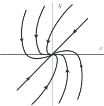
The origin is a center if α= 0, β 6= 0, (Figure 5).

x y

Figure 5: Center

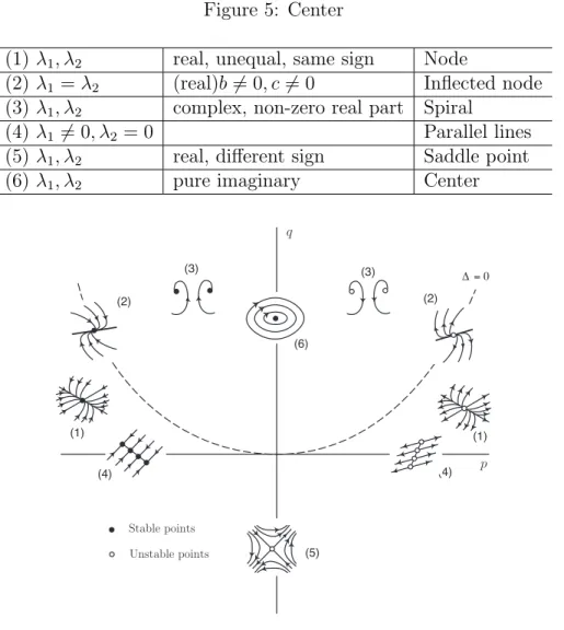
(1) λ1, λ2 real, unequal, same sign Node

(2) λ1 =λ2 (real)b6= 0, c6= 0 Inflected node

(3) λ1, λ2 complex, non-zero real part Spiral

(4) λ1 6= 0, λ2 = 0 Parallel lines

(5) λ1, λ2 real, different sign Saddle point

(6) λ1, λ2 pure imaginary Center

p q (6) (3) ₍₃₎ (2) (2) (1) (4) (4) (1) (5) Stable points Unstable points Δ = 0

Figure 6: General classification

Example. Classify the equilibrium point at (0,0) for the system

˙

Using Taylor expansion for the exponential function, the linearized system of equations about (0,0) is ˙ x=−x−3y, y˙ =−x, or in matrix form ˙ x ˙ y ! = −₋1_{1 0}−3 ! x y ! .

The eigenvalues are λ1,2 = −1±

√ 17

2 are real with different sign. The equi-librium is a saddle point.

5

Partial differential equations

The word “ordinary” in ordinary differential equation distinguishes it from partial differential equation(PDE), involves partial derivatives of two or more

independent variables. For a first order partial differential equation, a unified general theory exists; however, this a case for higher order partial differential equations. Generally speaking, the second order PDEs may be classified into three following categories, viz., elliptic, hyperbolic, and parabolic types.

5.1

Normal forms of elliptic, hyperbolic, and parabolic

Equations

Consider a linear second order differential operator for the function u(x, y) given by L(u) = a∂2u ∂x2 +b ∂2_u ∂x∂y +c ∂2_u ∂y2, (114)

wherea, b,andcare either constants or functions ofxandy. A corresponding quasilinear PDE may be represented by

L(u) +g(x, y, ∂u/∂x, ∂u/∂y) = L(u) +...= 0, (115) where g(x, y, ∂u/∂x, ∂u/∂y) is not necessarily linear and does not contain any second derivative.

Let us introduce the transformations

ξ =αx+βy,

η=γx+δy. (116)

Therefore, L(u) in Eq. (114) takes the form

L(u) = (aα2_+bαβ+cβ2₎∂2u ∂ξ2 +(2aαγ+b(αδ+βγ) + 2cβδ) ∂2u ∂ξ∂η +(aγ2_+bγδ+cδ2₎∂2u ∂η2 . (117)

If the transformed operator is desired to be of the form _∂ξ∂η∂2u , then we need

aα2_+bαβ+cβ2 _{= 0, (118)}

aγ2_+bγδ+cδ2 _{= 0. (119)}

If a = c= 0, then the trivial transformation ξ = y and η = y provides the desired form. For the non-trivial case eithera orcor both are non-zero. Let us say a6= 0, thereby implying that α6= 0, γ 6= 0. Dividing Eq. (118) by β2

and Eq. (119) by δ2_{, we obtain two quadratic equations in (α/β) and (γ/δ).}

These yield α/β= 1 2a{−b± √ b2 _{−4ac}, (120)} γ/δ= 1 2a{−b± √ b2_{−4ac}. (121)}

The ratios α/β and γ/δ must be different (by choosing positive sign in Eq. (120) and negative sign in Eq. (121)) so that the transformation given by Eq. (116) is non-singular. Further b2_{−4ac should be positive.}

Therefore,L(u) reduces to the form ∂2u

∂ξ∂η if and only if

and this case is said to be “hyperbolic”. Then the transformation Eq. (116) takes the form

ξ = (−b+√b2_{−4ac)x+ 2ay,}

η = (−b−√b2_{−4ac)x+ 2ay. (123)}

Then the PDE given by Eq. (115) reduces to −4a(b2_−4ac) ∂2u ∂ξ∂η +g(ξ, η, ∂u ∂ξ, ∂u ∂η) = 0. (124)

If b2 _{−4ac= 0, then L is termed as “parabolic”. In this case Eq. (120) and}

Eq. (121) reduce to a single equation andα/β =−b/2aforces the coefficient of ∂2_u/ξ2 _{in Eq. (117) to vanish. Further, sinceb}2 _{= 4ac orb/2a= 2c/b, the}

coefficient of _∂ξ∂η∂2u also vanish. Thus the transformation (c.f. Eq. (123))

ξ=−bx+ 2ay,

η=x (arbitrary), (125)

can be used to transform Eq. (115) into

a ∂2

∂η2 +g( ) = 0. (126)

This is the normal form of a parabolic quasilinear PDE.

For the final case, b2 _{−4ac < 0, and the operator L(u) is said to be}

“elliptic”. In this case it is not possible to eliminate the coefficients of ∂_∂ξ2u₂ or ∂_∂η2u₂. Nevertheless, if we use the transformation

ξ = √2ay−bx

4ac−b2, η=t (arbitrary), (127)

then L(u) =a ∂_∂ξ2u₂ + ∂_∂η2u₂ !

, and the general PDE has the form

a ∂2u ∂ξ2 + ∂2_u ∂η2 ! +g(ξ, η,∂u ∂ξ, ∂u ∂η) = 0. (128)

For the linear case

∂2_u

∂ξ2 +

∂2_u

∂η2 = 0, (129)

which is the well-known Laplace’s equation.

Once a PDE has been reduced to its normal form, the method of character-istic may be effectively used to find its solution.

However, in the following we discuss the solution of a particular hyperbolic equation, known as the “wave equation” by the use of “separation of the variables” which is a popular approach in engineering.

The equation

c2∂2u(x, t)

∂x2 −u¨(x, t) = 0, c= constant, (130)

is a partial differential equation. The following notation was used ¨

u(x, t) = ∂2u_∂t(x, t₂ ).

The initial conditions are

u(x,0) =f(x), u˙(x,0) =g(x). (131) The boundary conditions are

∂u

∂x(0, t) = ∂u

∂x(l, t) = 0. (132)

We seek the solution of Eq. (130) in the form of a product of a function of time and a function of position

u(x, t) = U(x)ϕ(t). (133)

Introducing (133) into (130), we replace Eq. (130) by the system of two ordinary equations

¨

ϕ+β2_c2_{ϕ= 0, (134)}

d2_U

where β is for the time being an undetermined parameter. The solution of Eqs. (134) and (135) is

ϕ(t) = Asinωt+Bcosωt, (136)

U(x) =Csinβx+Dcosβx, (137)

where ω =βc.

We first consider the second boundary conditions (132). They imply that

C = 0 and

Dβsinβl= 0.

The latter condition is satisfied if

βn = nπ_l , (n= 0,1,2, . . . ,∞). (138)

It is evident that every value of βn is associated with a particular solution of

Eq. (130), viz.

un(x, t) = (Ansinωnt+Bncosωnt)Dcosβnx. (139)

The general solution of (130) takes the form

u(x, t) = X∞ n=0 un(x, t) = ∞ X n=0

(Ansinωnt+Bncosωnt)Dcosβnx. (140)

The constants An, Bn are to be found from the initial conditions (131)

i.e. f(x) = ∞ X n=0DBncosβnx, g(x) = ∞ P n=0DωnAncosβnx. (141) The functions Un(x) = Dcosβnx, (142)

are the eigenfunctions of the problem. They are orthogonal, i.e.

l Z 0 Un(x)Um(x)dx = 0, if n6=m, l Z 0 U2 n(x)dx= ₂lD2, if n=m, (143)

as can easily be verified by integration. The constant D is arbitrary. Assume that D2 _{= 2/l. Then}Rl

0 U 2

n(x)dx= 1 and the eigenfunctions

Un(x) = s 2 l cosβnx= s 2 l cos nπx l , (144)

are called normalized eigenfunctions.

Making use of the normalized eigenfunctions we can rewrite relations (141) in the form f(x) = s 2 l ∞ X n=0Bncosβnx, g(x) = s 2 l ∞ X n=0ωnAncosβnx. (145)

To find the coefficient Bn we multiply the first equation (145) by cosβnx

and integrate with respect to xfrom 0 to l. Then, making use of the orthog-onality relations, we obtain

Bn= s 2 l l Z 0 f(x) cosβnx dx, (n= 1,2, . . . ,∞), B0 = 1₂ s 2 l l Z 0 f(x)dx. (146) Similarly we have An = _cβ1 n s 2 l l Z 0 g(x) cosβnx dx, (n= 1,2, . . . ,∞), A0 = 0. (147)

Introducing the values of An, Bn into Eq. (140), we arrive at the final

solution.

Example. We consider next the equation

c2∂2u

∂x2 −u¨= 0, (148)

with assuming homogeneous initial conditions (u(x,0) = ˙u(x,0) = 0) and the boundary conditions

Performing the Laplace transform in Eq. (148) for the above boundary con-ditions, we obtain c2d2u dx2 −s2u=−su(x,0)−u˙(x,0), (150) u(0, s) = 0;du_dx(l, s) =P(s), (151) where u(x, s) = ∞ Z 0 e−_{stu(x, t)dt, P(s) =} ∞ Z 0 e−_stP(t)dt.

The right-hand side of Eq. (150) vanishes in view of the homogeneous initial conditions, hence its solution can be represented in the form

u(x, s) = A(s)e−_{sx/c+B(s)esx/c. (152)}

The functionsA(s),B(s) can be determined by means of the boundary con-ditions (151): A(s) = −B(s), B(s) = P(s)c 2s coshsl c . (153) Hence u(x, s) = P(₂s)l esx/c_sl −e−sx/c c cosh sl c , i.e. u(x, s) = P(s)lsinh sx c sl c cosh sl c . (154)

Now we invert the Laplace transform in (154). Taking into account that

L−1     sinhsx_c scoshsl_c     = 2 π ∞ X n=1 (−1)n−₁ n− 1 2 sinn− 1₂πx_l sin " n− 1 2 πlt c # ,

and

L−1_{P(s) = P(t),}

and making use of the convolution theorem was obtain

u(x, t) = 2_πc X∞ n=1 (−1)n−₁ n−1 2 sinn− 1₂πx_l t Z 0 P(τ) sin " 2n−1 2 πl c(t−τ) # dτ. (155)

In the particular case

P(t) =P0H(t),

where H(t) is the Heaviside function, we have from Eq. (155)

u(x, t) = 8P0c2 π2_L ∞ X n=1 (−1)n−1 (2n−1)2 sin 2n−1 2 πx l " 1−cos(2n−_2c1)πlt # . (156)

Assume thatP(t) = P0eiωt acts at the end x= 0 of the fixed rod. Taking

into account that u(x, t) =U(x)eiωt_{, we transform Eq. (148) to the form}

c2d2U

dx2 +ω2U = 0. (157)

The boundary conditions take the form

U(0) = 0, dU

dx(l) = P0. (158)

The constantsA,B appearing in the solution

U(x) = Asinωx

c +Bcos ωx

of Eq. (157) are determined from the boundary conditions (158). Finally we obtain u(x, t) = P0ceiωt ω sinωx_c cosωl_c . (160)

If the frequencyωapproaches any of the eigenfrequency, the displacement

6

Applications

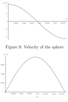
Problem 1. A sphere of mass m falls on a vertical spring as shown in

the Figure 7. The sphere makes contact with the spring and the spring compresses. The compression phase ends when the velocity of the sphere is zero. Next phase is the restitution phase when the spring is expanding and the sphere is moving upward. At the end of the restitution phase there is the separation of the sphere.

Find and solve the equation of motion for the sphere in contact with the spring.

x O

h

Figure 7: Sphere in contact with a spring

Solution

The x-axis selected downward as shown in the Figure 7.

At the moment t = 0 it is assumed that the sphere gets in contact with the spring and has the velocity v(t = 0) =v₀ =v₀ı.

Using Newton’s second law, the equation of motion for the sphere in contact with the spring is:

ma=G+F_e or mx¨=m g−k x. (161)

The acceleration of the sphere is a= ¨xı, where x is the linear displacement.

The weight of the sphere is G=m gı, whereg is the gravitational

of the spring. The initial conditions are

x(0) = 0 and ˙x(0) =v0.

With the notation

k

m =ω2, (ω >0),

Equation (161) becomes

¨

x+ω2_{x=g. (162)}

Assume the solution of Eq. (162) has the following expression

x=a cos(ω t−ϕ0) +b. (163)

Then ˙

x=−a ω sin(ω t−ϕ0) and ¨x=−a ω2 cos(ω t−ϕ0).

Substituting Eq. (164) into Eq. (162) −a ω2 _{cos(ω t−ϕ}

0) +ω2[a cos(ω t−ϕ0) +b] =g,

the constant b is obtained

b= g

ω2. (164)

Using the initial conditions (x(0) = 0 and ˙x(0) =v0) the following expressions

are obtained

x(0) =a cos(−ϕ0) +b=a cosϕ0+b= 0,

˙

x(0) =−a ω sin(−ϕ0) =a ωsinϕ0 =v0,

or

a cosϕ0 =−b =−_ωg₂ and a sinϕ0 = v_ω0.

It results a= s g2 ω4 + v2 0 ω2, tan ϕ0 =−v0_gω or ϕ0 =−arctanv0_gω. (165)