Cross-correlation of weak lensing and gamma rays: implications for the
nature of dark matter
Tilman Tr¨oster,
1‹Stefano Camera,
2Mattia Fornasa,
3Marco Regis,
4,5Ludovic van Waerbeke,
1Joachim Harnois-D´eraps,
6Shin’ichiro Ando,
3Maciej Bilicki,
7Thomas Erben,
8Nicolao Fornengo,
4,5Catherine Heymans,
6Hendrik Hildebrandt,
8Henk Hoekstra,
7Konrad Kuijken
7and Massimo Viola
71Department of Physics and Astronomy, The University of British Columbia, 6224 Agricultural Road, Vancouver, B.C., V6T 1Z1, Canada 2Jodrell Bank Centre for Astrophysics, The University of Manchester, Alan Turing Building, Oxford Road, Manchester M13 9PL, UK
3Gravitation Astroparticle Physics Amsterdam (GRAPPA), University of Amsterdam, Science Park 904, NL-1098 XH Amsterdam, the Netherlands 4Dipartimento di Fisica, Universit`a di Torino, via P. Giuria 1, I-10125 Torino, Italy
5Istituto Nazionale di Fisica Nucleare, Sezione di Torino, via P. Giuria 1, I-10125 Torino, Italy
6Institute for Astronomy, University of Edinburgh, Royal Observatory, Blackford Hill, Edinburgh EH9 3HJ, UK 7Leiden Observatory, Leiden University, PO Box 9513, NL-2300 RA Leiden, the Netherlands
8Argelander-Institut f¨ur Astronomie, Auf dem H¨ugel 71, D-53121 Bonn, Germany
Accepted 2017 February 8. Received 2017 February 3; in original form 2016 November 23
A B S T R A C T
We measure the cross-correlation betweenFermigamma-ray photons and over 1000 deg2of
weak lensing data from the Canada–France–Hawaii Telescope Lensing Survey (CFHTLenS), the Red Cluster Sequence Lensing Survey (RCSLenS), and the Kilo Degree Survey (KiDS). We present the first measurement of tomographic weak lensing cross-correlations and the first application of spectral binning to cross-correlations between gamma rays and weak lensing. The measurements are performed using an angular power spectrum estimator while the covariance is estimated using an analytical prescription. We verify the accuracy of our covariance estimate by comparing it to two internal covariance estimators. Based on the non-detection of a cross-correlation signal, we derive constraints on weakly interacting massive particle (WIMP) dark matter. We compute exclusion limits on the dark matter annihilation cross-sectionσannv, decay ratedecand particle massmDM. We find that in the absence of
a cross-correlation signal, tomography does not significantly improve the constraining power of the analysis. Assuming a strong contribution to the gamma-ray flux due to small-scale clustering of dark matter and accounting for known astrophysical sources of gamma rays, we exclude the thermal relic cross-section for particle masses ofmDM20 GeV.
Key words: gravitational lensing: weak – dark matter – gamma-rays: diffuse background.
1 I N T R O D U C T I O N
The matter content of the Universe is dominated by so-called dark matter whose cosmological abundance and large-scale clustering properties have been measured to high precision (e.g. Hinshaw et al. 2013; Anderson et al.2014; Hoekstra et al. 2015; Mantz et al.2015; Ross et al.2015; Hildebrandt et al.2017; Planck Collab-oration XIII2016). However, little is known about its microscopic nature, beyond its lack of – or at most weak – non-gravitational interaction with standard model matter.
E-mail:[email protected]
Weakly interacting massive particles (WIMPs) thermally pro-duced in the early Universe are among the leading dark matter candidates. With a mass of the order of GeV/TeV, their decoupling from thermal equilibrium occurs in the non-relativistic regime. The weak interaction rate with lighter standard model particles further-more ensures that their thermal relic density is naturally of the order of the measured cosmological dark matter abundance (Lee & Weinberg1977; Gunn et al.1978).
Many extensions of the standard model of particle physics pre-dict the existence of new massive particles at the weak scale; some of these extra states can indeed be ‘dark’, i.e. be colour and electromagnetic neutral, with the weak force and grav-ity as the only relevant coupling to ordinary matter (for re-views, see e.g. Jungman, Kamionkowski & Griest1996; Bertone,
C
Hooper & Silk2005; Schmaltz & Tucker-Smith2005; Hooper & Profumo2007; Feng2010).
The weak coupling allows us to test the hypothesis of WIMP dark matter: supposing that WIMPs are indeed the building blocks of large-scale structure (LSS) in the Universe, there is a small but finite probability that WIMPs in dark matter haloes annihilate or decay into detectable particles. These standard model particles produced by these annihilations or decays would manifest as cosmic rays which can be observed. In particular, since the WIMP mass is around the electroweak scale, gamma rays can be produced, which can be observed with ground-based or space-borne telescopes, e.g. theFermitelescope (Atwood et al.2009). Indeed, analyses of the gamma-ray sky have already been widely used to put constraints on WIMP dark matter [see e.g. Charles et al. (2016) for a recent review].
The currently strongest constraints on the annihilation cross-section and WIMP mass come from the analysis of local regions with high dark matter content, such as dwarf spheroidal galaxies (dSphs) (Ackermann et al.2015b). These analyses exclude anni-hilation cross-sections larger than∼3× 10⁻²⁶cm3s−1 for dark
matter candidates lighter than 100 GeV. This value for the annihila-tion cross-secannihila-tion is known as the thermal cross-secannihila-tion and, below it, many models of new physics predict dark matter candidates that yield a relic dark matter density in agreement with cosmological measurements of the dark matter abundance (Jungman et al.1996). Instead of these local probes of dark matter properties, one could consider the unresolved gamma-ray background (UGRB), i.e. the cumulative radiation produced by all sources that are not bright enough to be resolved individually. Correctly modelling the contri-bution of astrophysical sources, such as blazars, star-forming and radio galaxies, allows the measurement of the UGRB to be used to constrain the component associated with dark matter (Fornasa & S´anchez-Conde2015). Indeed, the study of the energy spectrum of the UGRB (Ackermann et al.2015a), as well as of its anisotropies (Ando & Komatsu2013; Fornasa et al.2016) and correlation with tracers of LSS (Ando, Benoit-L´evy & Komatsu2014; Shirasaki, Horiuchi & Yoshida2014; Cuoco et al.2015; Fornengo et al.2015; Regis et al.2015; Shirasaki, Horiuchi & Yoshida 2015; Ando & Ishiwata2016; Feng, Cooray & Keating2017; Shirasaki et al.2016) have yielded independent and competitive constraints on the nature of dark matter.
In this paper, we focus on the cross-correlation of the UGRB with weak gravitational lensing. Gravitational lensing is an unbi-ased tracer of matter and thus closely probes the distribution of dark matter in the Universe. This makes it an ideal probe to cross-correlate with gamma rays to investigate the particle nature of dark matter (Camera et al.2013).
We extend previous analyses of cross-correlations of gamma rays and weak lensing of Shirasaki et al. (2014,2016) by adding weak lensing data from the Kilo Degree Survey (KiDS) (de Jong et al.2013; Kuijken et al.2015) and making use of the spectral and tomographic information contained within the data sets. This paper presents the first tomographic weak lensing cross-correlation mea-surement and the first application of spectral binning to the cross-correlation between gamma rays and galaxy lensing. Exploiting tomography and the information contained in the energy spectrum of the dark matter annihilation signal has been shown to greatly increase the constraining power compared to the case where no binning in redshift or energy is performed (Camera et al.2015).
The structure of this paper is as follows: in Section 2 we introduce the formalism and theory; the data sets are described in Section 3; Section 4 introduces the measurement methods and estimators; the
results are presented in Section 5; and we draw our conclusions in Section 6.
2 F O R M A L I S M
Our theoretical predictions are obtained by computing the angular cross-power spectrumCgκbetween the lensing convergenceκand gamma-ray emissions for different classes of gamma-ray sources, denoted byg. In the Limber approximation (Limber1953), it takes the form Cgκ = E dE ∞ 0
dz c
H(z) 1
χ(z)2
×Wg(E, z)Wκ(z)Pgδ
k=
χ(z), z
, (1)
wherez is the redshift,E is the gamma-ray energy andEthe energy bin that is being integrated over,cis the speed of light in the vacuum,H(z) is the Hubble rate, andχ(z) is the comoving distance. We employ a flatCDM cosmological model with parameters taken from Planck Collaboration XIII (2016).
WgandWκ are the window functions that characterize the
red-shift and energy dependence of the gamma-ray emitters and the efficiency of gravitational lensing, respectively.Pgδ(k,z) is the
three-dimensional cross-power spectrum between the gamma-ray emis-sion for a gamma-ray source class and the matter densityδ, withk
being the modulus of the wavenumber andthe angular multipole. The functional form of the window functions and power spectra de-pend on the populations of gamma-ray emitters and source galaxy distributions under consideration and are described in the following subsections.
The quantity measured from the data is the tangential shear cross-correlation functionξgγt(ϑ). This correlation function is related to the angular cross-power spectrum by a Hankel transformation:
ξgγt(ϑ)= 1 2π
∞
0
d J2(ϑ)Cgκ , (2)
whereϑis the angular separation in the sky andJ2is the Bessel
function of the first kind of the order of 2.
2.1 Window functions
The window function describes the distribution of the signal along the line of sight, averaged over all lines of sight.
2.1.1 Gravitational lensing
For the gravitational lensing the window function is given by (see, e.g. Bartelmann2010)
Wκ(z)= 3 2H
2
0M(1+z)χ(z)
∞
z
dzχ(z )−χ(z)
χ(z) n(z
), (3)
whereH0is the Hubble rate today,Mis the current matter
abun-dance in the Universe, and n(z) is the redshift distribution of background galaxies in the lensing data set. The galaxy distribu-tion depends on the data set and redshift selecdistribu-tion, as described in Section 3.1. The redshift distribution functionn(z) is binned in redshift bins of widthz=0.05. To compute the window function
Figure 1. Top: window functions for the gamma-ray emissionsWg for the energy range 0.5–500 GeV and redshift selection of 0.1–0.9. Shown are the window functions for the three annihilating dark matter scenarios considered, i.e.HIGH(blue),MID(purple),LOW(red); decaying dark matter (black); and the sum of the astrophysical sources (green). The annihilation scenarios assumemDM=100 GeV andσannv =3×10⁻²⁶cm3s−1. For decaying dark matter,mDM =200 GeV anddec=5×10⁻²⁸s−1. The predictions for annihilating and decaying dark matter are for thebb¯channel. We consider three populations of astrophysical sources that contribute to the UGRB: blazars, mAGNs and SFGs, described in Section 2.1.3. Bottom: the lensing window functions for the five tomographic bins chosen for KiDS.
2.1.2 Gamma-ray emission from dark matter
We consider two processes by which dark matter can create gamma rays: annihilation and decay.
The window function for annihilating dark matter reads (Ando & Komatsu2006; Fornengo & Regis2014)
Wgann(z, E)=
(DMρc)2 4π
σannv
2mDM2
(1+z)32(z)
×dNann
dE [E(1+z)] e
−τ[z,E(1+z)],
(4)
whereDMis the cosmological abundance of dark matter,ρcis the
current critical density of the Universe,mDMis the rest mass of the
dark matter particle, andσannvdenotes the velocity-averaged
an-nihilation cross-section, assumed here to be the same in all haloes. dNann/dE indicates the number of photons produced per
annihi-lation as a function of photon energy, and sets the gamma-ray energy spectrum. We will consider it to be given by the sum of two contributions: prompt gamma-ray production from dark mat-ter annihilation, which provides the bulk of the emission at low masses, and inverse Compton scattering of highly energetic dark matter-produced electrons and positrons on CMB photons, which upscatter in the gamma-ray band. The final states of dark matter annihilation are computed by means of the PYTHIAMonte Carlo
package v8.160 (Sj¨ostrand, Mrenna & Skands2008). The inverse Compton scattering contribution is calculated as in Fornasa et al. (2013), which assumes negligible magnetic field and no spatial dif-fusion for the produced electrons and positrons. Results will be shown for three final states of the annihilation: bb¯ pairs, which yields a relatively soft spectrum of photons and electrons, mostly
associated with hadronization into pions and their subsequent de-cay;μ+μ−, which provides a relatively hard spectrum, mostly as-sociated with final state radiation of photons and direct decay of the muons into electrons; andτ+τ−, which is in between the first two cases, being a leptonic final state but with semi-hadronic decay into pions (Fornengo, Pieri & Scopel2004; Cembranos et al.2011; Cirelli et al.2011).
The optical depth τ in equation (4) accounts for attenuation of gamma rays due to scattering off the extragalactic background light (EBL), and is taken from Franceschini, Rodighiero & Vaccari (2008).
The clumping factor2 is related to how dark matter density
is clustered in haloes and subhaloes. Its definition depends on the square of the dark matter density; therefore, it is a measure of the amount of annihilations happening and, thus, the expected gamma-ray flux. The clumping factor is defined as (see, e.g. Fornengo & Regis2014)
2(z)≡ ρ 2 DM
¯
ρ2 DM
= Mmax
Mmin
dMdnh
dM(M, z) [1+bsub(M, z)]
×
d3xρ
2 h(x|M, z)
¯
ρ2 DM
, (5)
where ¯ρDMis the current mean dark matter density, dnh/dMis the
halo mass function (Sheth & Tormen1999),Mminis the minimal halo
mass (taken to be 10−6M ),M
maxis the maximal mass of haloes
(for definiteness, we use 1018M , but the results are insensitive to
the precise value assumed),ρh(x|M, z) is the dark matter density
profile of a halo with massMat redshiftz, taken to follow a Navarro– Frenk–White (NFW) profile (Navarro, Frenk & White1997), and
bsubis the boost factor that encodes the ‘boost’ to the halo emission
provided by subhaloes. To characterize the halo profile and the subhalo contribution, we need to specify their mass concentration. Modelling the concentration parameterc(M,z) at such small masses and for subhaloes is an ongoing topic of research and is the largest source of uncertainty of the models in this analysis. We consider three cases:LOW, which uses the concentration parameter derived in
Prada et al. (2012) (see also S´anchez-Conde & Prada2014);HIGH,
based on Gao et al. (2012); andMID, following the recent analysis of Molin´e et al. (2017). The last one represents our reference case with predictions that are normally intermediate between those of theLOWandHIGH. The authors in Molin´e et al. (2017) refined the
estimation of the boost factor of S´anchez-Conde & Prada (2014) by modelling the dependence of the concentration of the subhaloes on their position in the host halo. Accounting for this dependence and related effects, such as tidal stripping, leads to an increase of a factor of∼1.7 in the overall boost factor over theLOW model.
Predictions for the dark matter clumping factor for the three models are shown in Fig.2.
Since the number of subhaloes and, therefore, the boost fac-tor increases with increasing host halo mass, the integral in equation (5) is the dominated group and cluster-sized haloes (Ando & Komatsu2013). However, in the absence of subhaloes, the clump-ing factor in equation (5) would strongly depend on the low-mass cutoffMmin. The minimum halo massMmin depends on the
free-streaming scale of dark matter, which is assumed to be in the range of 10−12–10−3M (Profumo, Sigurdson & Kamionkowski2006;
Bringmann2009). We therefore choose an intermediary-mass cut-off ofMmin =10−6M . As all our models include substructure,
the dependence onMminis at mostO(1) (see e.g. fig. S3 in Regis
Figure 2. Dark matter clumping factor2, as defined in equation (5), as a function of redshift for theLOW(dash–dotted red),MID(dashed purple) and HIGH(solid blue) scenarios. TheMIDmodel is built from its expression at z=0 in Molin´e et al. (2017), assuming the same redshift scaling as in Prada et al. (2012).
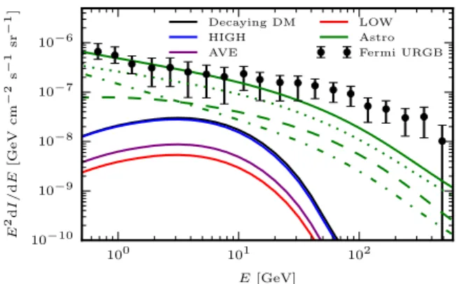
Figure 3. Intensities of the gamma-ray source classes considered in this work: annihilating dark matter assumingHIGH(solid blue),MID(solid purple), LOW(solid red) clustering models; decaying dark matter (solid black); and astrophysical sources (solid green). The dark matter particle properties are the same as in Fig.1. The astrophysical sources are further divided into blazars (dashed green), mAGN (dotted green) and SFG (dash–dotted green). The black data points represent the observed isotropic component of the UGRB (Ackermann et al.2015c).
The window function of decaying dark matter is given by (Ando & Komatsu2006; Ibarra, Tran & Weniger2013; Fornengo & Regis2014)
Wgdec(z, E)= DMρc
4π
dec mDM
dNdec
dE [E(1+z)] e
−τ[z,E(1+z)], (6)
wheredecis the decay rate anddNdEdec(E)= dNdEann(2E), i.e. the
en-ergy spectrum for decaying dark matter, is the same as that for an-nihilating dark matter described above, at twice the energy (Cirelli et al.2011). Unlike annihilating dark matter, decaying dark matter does not depend on the clumping factor and the expected emis-sion is thus much less uncertain. A set of representative window functions for annihilating and decaying dark matter is shown in the top panel of Fig.1. In Fig.3 we show the average all-sky gamma-ray emission expected from annihilating dark matter for the three clumping scenarios described above and from decaying dark matter.
2.1.3 Gamma-ray emission from astrophysical sources
Besides dark matter, gamma rays are produced by astrophysi-cal sources which will contaminate, and even dominate over the
expected dark matter signal. Indeed, astrophysical sources have been shown to be able to fully explain the observed cross-correlations between gamma rays and tracers of LSS, like galaxy catalogues (Cuoco et al.2015; Xia et al. 2015). For this analy-sis, we model three populations of astrophysical sources of gamma rays: blazars, misaligned active galactic nuclei (mAGNs) and star-forming galaxies (SFGs). The sum of the gamma-ray emissions produced by the three extragalactic astrophysical populations de-scribed above approximately accounts for all the UGRB measured (see Fornasa & S´anchez-Conde 2015), as shown Fig. 3, where the emissions from the three astrophysical source classes are com-pared to the most recent measurement of the UGRB energy spec-trum from Ackermann et al. (2015c). For each of these astrophys-ical gamma-ray sources, we consider a window function of the form
WgS(z, E)=χ(z)
2
Lmax(Fsens,z)
Lmin
dLdF
dE(L, z)(L, z), (7)
where L is the gamma-ray luminosity in the energy interval 0.1–100 GeV, andis the gamma-ray luminosity function (GLF) corresponding to one of the source classes of astrophysical emitters included in our analysis. The upper bound,Lmax(Fsens, z), is the
lu-minosity above which an object can be resolved, given the detector sensitivityFsens, taken from Ackermann et al. (2015d). As we are
in-terested in the contribution from unresolved astrophysical sources, only sources with luminosities smaller thanLmaxare included.
Con-versely, the minimum luminosityLmindepends on the properties of
the source class under investigation. The differential photon flux is given by dF/dE=dNS/dE×e−τ[z,E(1+z)], where dNS/dEis the
observed energy spectrum of the specific source class and the ex-ponential factor again accounts for the attenuation of high-energy photons by the EBL.
We consider a unified blazar model combining BL Lacertae and flat-spectrum radio quasars as a single source class. The GLF and energy spectrum are taken from Ajello et al. (2015) where they are derived from a fit to the properties of resolved blazars in the third
Fermi-LAT catalogue (Acero et al.2015).
In the case of mAGN, we follow Di Mauro et al. (2014), who studied the correlation between the gamma-ray and radio luminosity of mAGN, and derived the GLF from the radio luminosity function. We consider their best-fittingL–Lr,corerelation and assume a
power-law spectrum with indexαmAGN=2.37.
To build the GLF of SFG, we start from the IR luminosity function of Gruppioni et al. (2013) (adding up spiral, starburst and SF-AGN populations of their table 8) and adopt the best-fittingL–LIRrelation
from Ackermann et al. (2012). The energy spectrum is taken to be a power law with spectral indexαSFG=2.7.
The window function and average all-sky emission expected from the astrophysical sources are shown as green lines in the top panel of Figs1and3, respectively.
2.2 Three-dimensional power spectrum
The three-dimensional cross-power spectrum Pgδ between the gamma-ray emission of a source class gand the matter density is defined as
fˆg(z,k) ˆf∗
δ(z,k) =(2π)3δ3(k+k)Pgδ(k, z, z), (8)
density of gamma-ray emission due to decaying dark matter traces the dark matter density contrastδDM, while the emission associated
with annihilating dark matter tracesδ2
DM. Astrophysical sources are
assumed to be point-like biased tracers of the matter distribution. Finally, lensing directly probes the matter contrastδM. To compute Pgδ, we follow the halo model formalism (for a review, see e.g.
Cooray & Sheth2002), and writeP= P1h+ P2h. We derive the
one-halo termP1hand the two-halo termP2has in Fornengo et al.
(2015) and in Camera et al. (2015).
2.2.1 Dark matter gamma-ray sources
The 3D cross-power spectrum between dark matter sources of gamma rays and matter density is given by:
P1h
gDMκ(k, z)= Mmax
Mmin
dM dnh
dM(M, z) ˆvgDM(k|M, z) ˆuκ(k|M, z)
P2h
gDMκ(k, z)= Mmax
Mmin
dM dnh
dM(M, z)bh(M, z) ˆvgDM(k|M, z)
× Mmax
Mmin
dM dnh
dM(M, z)bh(M, z) ˆuκ(k|M, z)
×Plin
(k, z), (9)
where Plin is the linear matter power spectrum, b
h is the
lin-ear bias (taken from the model of Sheth & Tormen 1999) and ˆuκ(k|M, z) is the Fourier transform of the matter halo density profile, i.e. ρh(x|M, z)/ρ¯DM. The Fourier transform of the gamma-ray emission profile for dark matter haloes is de-scribed by ˆvgDM(k|M, z). For decaying dark matter, ˆvgDM=uˆκ, i.e. the emission follows the dark matter density profile. Conversely, the emission for annihilating dark matter follows the square of the dark matter density profile: ˆvgDM(k|M, z)=uˆann(k|M, z)/(z)
2,
where ˆuann is the Fourier transform of the square of the main
halo density profile plus its substructure contribution, and (z)2
is the clumping factor. The mass limits areMmin=10−6M and Mmax=1018M again.
2.2.2 Astrophysical gamma-ray sources
The cross-correlation of the convergence with astrophysical sources is sourced by the 3D power spectrum
P1h
gSκ(k, z)= Lmax
Lmin
dL(L, z) fS
dF
dE(L, z) ˆuκ(k|M(L, z), z)
P2h
gSκ(k, z)= Lmax
Lmin
dLbS(L, z) i(L, z)
fS
dF dE(L, z)
× Mmax
Mmin
dM dnh
dMbh(M, z) ˆuκ(k|M, z)
×Plin(k, z), (10)
wherebSis the bias of gamma-ray astrophysical sources with respect
to the matter density, for which we adoptbS(L, z)=bh(M(L, z)).
That is, a source with luminosity L has the same bias bh as a
halo with mass M, with the relation M(L, z) between the mass of the host halo M and the luminosity of the hosted object L taken from Camera et al. (2015). The mean flux fSis defined
asfS =
dLdF
dE.
3 DATA
3.1 Weak lensing data sets
For this study we combine CFHTLenS1and RCSLenS2data sets
from the Canada–France–Hawaii Telescope (CFHT) and KiDS3
from the VLT Survey Telescope (VST), all of which have been optimized for weak lensing analyses. The same photometric redshift and shape measurement algorithms have been used in the analysis of the three surveys. However, there are slight differences in the algorithm implementation and in the shear and photometric redshift calibration, as described in the following subsections.
The sensitivity of the measurement depends inversely on the overlap area between the gamma-ray map and the lensing data, with a weaker dependence on the parameters characterizing the lensing sensitivity, i.e. the galaxy number density and elliptic-ity dispersion. This is due to the fact that at large scales, sam-pling variance dominates the contribution of lensing to the co-variance and reducing the shape noise does not result in an improvement of the overall covariance. This point is further discussed in Section 4.2.1.
Of the three surveys, only CFHTLenS and KiDS have full pho-tometric redshift coverage. We choose to restrict the tomographic analysis to KiDS, as the much smaller area of CFHTLenS is ex-pected to yield a much lower sensitivity for this measurement. In Section 5.2 we find that tomography does not appreciably improve the exclusion limits on the dark matter parameters. We thus do not lose sensitivity by restricting the tomographic analysis to KiDS in this work.
3.1.1 CFHTLenS
CFHTLenS spans a total area of 154 deg2from a mosaic of 171
in-dividual MEGACAM pointings, divided into four compact regions (Heymans et al.2012). Details on the data reduction are described in Erben et al. (2013). The observations in the five bandsugrizof the survey allow for the precise measurement of photometric redshifts (Hildebrandt et al.2012). The shape measurement withLENSFITis
described in detail in Miller et al. (2013). We make use of all fields in the data set as we are not affected by the systematics that lead to field rejections in the cosmic shear analyses (Kilbinger et al.2013). We correct for the additive shear bias for each galaxy individually, while the multiplicative bias is accounted for on an ensemble basis, as described in Section 4.1.
Individual galaxies are selected based on the Bayesian photo-metric redshiftzBbeing in the range [0.2, 1.1]. The resulting
red-shift distribution of the selected galaxies is obtained by stacking the redshift probability distribution function of individual galaxies, weighted by theLENSFITweight. As a result of the stacking of the
individual redshift PDFs, the true redshift distribution leaks outside thezBselection range. Stacking the redshift PDFs can lead to
bi-ased estimates of the true redshift distribution of the source galaxies (Choi et al.2016) but in light of the large statistical and modelling uncertainties in this analysis these biases can be safely neglected here.
3.1.2 RCSLenS
The RCSLenS data consist of 14 disconnected regions whose com-bined total area reaches 785 deg2. A full survey and lensing
anal-ysis description is given in Hildebrandt et al. (2016). RCSLenS uses the sameLENSFITversion as CFHTLenS but with a different
size prior, as galaxy shapes are measured fromi-band images in CFHTLenS, whereas RCSLenS uses therband. The additive and multiplicative shear biases are accounted for in the same fashion as in CFHTLenS.
Multi-band photometric information is not available for the whole RCSLenS footprint, therefore we use the redshift distri-bution estimation technique described in Harnois-D´eraps et al. (2016) and Hojjati et al. (2016). Of the three magnitude cuts con-sidered in Hojjati et al. (2016), we choose to select the source galaxies such that 18<magr <26, as this selection yielded the
strongest cross-correlation signal in Hojjati et al. (2016). This cut is close to the 18 < magr < 24 in Harnois-D´eraps et al.
(2016) but with the faint cutoff determined by the shape mea-surement algorithm. The redshift distribution is derived from the CFHTLenS-VIPERS sample (Coupon et al. 2015), a UV and IR extension of CFHTLenS. We stack the redshift PDF in the CFHTLenS-VIPERS sample, accounting for the RCSLenS magni-tude selection,r-band completeness and galaxy shape measurement (LENSFIT) weights.
3.1.3 KiDS
The third data set considered here comes from the KiDS, which currently covers 450 deg2with completeugrifour band photometry
in five patches. Galaxy shapes are measured in therband using the new self-calibratingLENSFIT(Fenech Conti et al.2016).
Cross-correlation studies such as this work are only weakly sensitive to additive biases and, being linear in the shear, are less affected by multiplicative biases than cosmic shear studies. Nonetheless, the analysis still benefits from well-calibrated shape measurements. The residual multiplicative shear bias is accounted for on an en-semble basis, as for CFHTLenS and RCSLenS. To correct for the additive bias we subtract theLENSFITweighted ellipticity means in
each tomographic bin. A full description of the survey and data products is given in Hildebrandt et al. (2017).
We select galaxies with 0.1≤zB<0.9 and then further split the
data into four tomographic bins [0.1, 0.3], [0.3, 0.5], [0.5, 0.7] and [0.7, 0.9]. We derive the effectiven(z) following the DIR method introduced in Hildebrandt et al. (2017).
3.2 Fermi-LAT
For this work we useFermidata gathered until 2016 September 1, spanning over eight years of observations. We use Pass 8 event reconstruction and reduce the data using FERMI SCIENCE TOOLS
version v10r0p5. We select FRONT+BACK converting events (evtype=3) between energies of 0.5 and 500 GeV. We restrict our main analysis toultracleanvetophotons (evclass=1024). We verify that selecting clean photons (evclass=256) does not change the results of the analysis. Furthermore, we apply the cuts (DATA_QUAL>0)&&(LAT_CONFIG==1) on the data quality. We then create full sky HEALPIX4
4http://healpix.sourceforge.net/
photon count and exposure maps with nside=1024 (G´orski et al.2005) in 20 logarithmically spaced energy bins in the range mentioned above.
The flux map used in the cross-correlation analysis is obtained by dividing the count maps by the exposure maps in each energy bin before adding them. We have confirmed that the energy spectrum of the individual flux maps follows a broken power law with an index of 2.34±0.02, consistent with that obtained in previous studies of the UGRB (Ackermann et al.2015a).
We also create maps for four energy bins 0.5–0.766 GeV, 0.766– 1.393 GeV, 1.393–3.827 GeV and 3.827–500 GeV. The bins are chosen such that they would contain equal photon counts for a power-law spectrum with index 2.5. The flux maps for the four energy bins are computed by first dividing each energy bin into three logarithmically spaced bins, creating flux maps for these fine bins, and then adding them up.
The total flux is dominated by resolved point sources and, to a lesser extent, by diffuse Galactic emissions. To probe the unre-solved component of the gamma-ray sky, we mask the 500 bright-est point sources in the thirdFermipoint source catalogue (Acero et al. 2015) with circular masks with a radius of two degrees. The remaining point sources are masked with one degree circu-lar masks. We checked that the analysis is robust with respect to other masking strategies. The effect of the diffuse Galactic emis-sion (DGE) is minimized by subtracting thegll_iem_v06model. Furthermore, we employ a 20◦cut in Galactic latitude. It has been shown in Shirasaki et al. (2016) that this cross-correlation anal-ysis is robust against the choice made for the model of DGE. We have confirmed that our results are not significantly affected even in the extreme scenario of not removing the DGE at all. This represents an important benefit of using cross-correlations to study the UGRB over studies of the energy spectrum alone, as in Ackermann et al. (2015a).
The robustness of these selection and cleaning choices is demon-strated in Fig.A3, where the impact of the event selection, point source masks and cleaning of the DGE on the cross-correlation sig-nal is shown. None of these choices leads to a significant change in the measured correlation signal, highlighting the attractive feature of cross-correlation analyses that uncorrelated quantities, such as Galactic emissions and extragalactic effects like lensing, do not bias the signal.
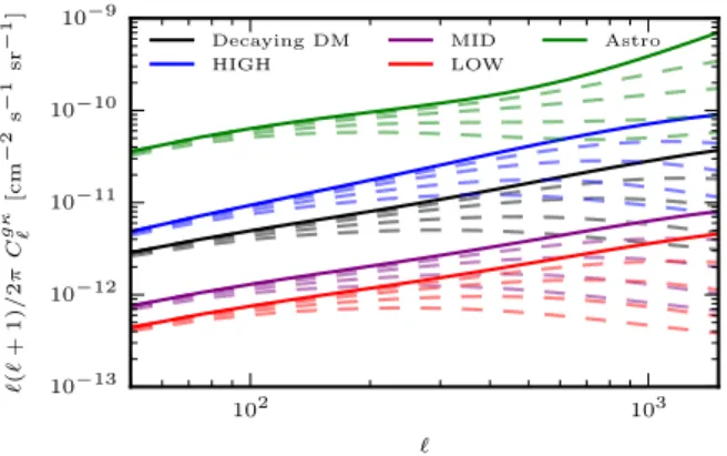
The point spread function (PSF) ofFermiis energy dependent and, especially at low energies, significantly reduces the cross-correlation signal power at small angular scales, as demonstrated in Fig.4. The pixelation of the gamma-ray sky has a similar but much weaker effect. In this analysis, we choose to account for this suppression of power by forward modelling. That is, rather than correcting the measurements, the predicted angular power spectra
Cgκ are modified to account for the effect of the PSF and pixel window function.
The gamma-ray data used in the analysis are obtained by cutting out regions around the lensing footprints. To increase the sensitivity at large angular scales, we include an additional four degree wide band around each of the 23 lensing patches.
4 M E T H O D S
4.1 Estimators
Figure 4. ModelCgκfor three annihilating dark matter scenarios, decaying dark matter and astrophysical sources. The models and formatting are the same as in Figs1and3. The models assume then(z) for thez∈[0.1, 0.9] bin for KiDS and the energy range 0.5–500 GeV. The dashed lines indicate the effect of theFermiPSF on the cross-power spectrum for the four energy bins, with the lowest energy bin having the strongest suppression of power at small scales. For clarity, the effect of the PSF for the different energy bins is shown on the cross-power spectrumCgκ for the single energy bin of 0.5–500 GeV.
et al.2014; Harnois-D´eraps et al.2016; Hojjati et al.2016):
ˆ
ξgγt/x(ϑ)=
ijwiet/xij gjij(ϑ)
ijwiij(ϑ) 1 1+K(ϑ),
1 1+K(ϑ) =
ijwiij(ϑ)
ijwi(1+mi)ij(ϑ),
(11)
where the sum runs over all galaxiesiand pixelsjof the gamma-ray flux map,wiis theLENSFIT-weight of galaxyiandet/xij is the
tangential (t) or cross (x) component of the shear with respect to the position of pixelj,gjis the flux at pixelj, andij(ϑ) accounts
for the angular binning, being equal to 1 if the distance between galaxyiand pixeljfalls within the angular bin centred onϑand 0 otherwise. The factor of 1
1+K accounts for the multiplicative shear bias, withmibeing the multiplicative shear bias of galaxyi.
The ˆξgγt/x(ϑ) measurement described with equation (11) exhibits strong correlation between the angular bins at all scales. This com-plicates the estimation of the covariance matrix as the off-diagonal elements have to be estimated accurately. On the other hand, the covariance of the angular cross-power spectrum ˆCgκis largely di-agonal since the measurement is noise-dominated. We thus choose to work with angular power spectrum ˆCgκ instead of the correla-tion funccorrela-tion ˆξgγt(ϑ). Inverting the relation in equation (2), one can construct an estimator for the angular cross-power spectrum
ˆ
Cgκ based on the measurement of ˆξgγt(ϑ) (Szapudi et al.2001; Schneider et al.2002). Specifically, working in the flat-sky approx-imation, one can write
ˆ
Cgκ =2π ∞
0
dϑ ϑJ2(ϑ) ˆξgγt(ϑ). (12)
This estimator yields an estimate for the cross-power spectrum be-tween the gamma rays and the E mode of the shear field. Replacing the tangential shearγtin equation (12) with the cross-component
of the shear γx results in an estimate of the cross-power
spec-trum between the gamma rays and the B mode of the shear field, which is expected to vanish in the absence of lensing systematics. In Appendix A, we check that this estimator indeed accurately recovers the underlying power spectrum.
To estimate the power spectrum using estimator in equation (12), we measure the tangential shear between 1 and 301 arcmin in 300
linearly spaced bins. The resulting power spectrum is then binned in five linearly spaced bins betweenof 200 and 1500. At smaller scales the FermiPSF suppresses power, especially at low ener-gies. At very large scales of100, the covariance is affected by residuals from imperfect foreground subtraction, hence we restrict ourselves to scales of >200.
4.2 Covariances
Our primary method to estimate the covariance relies on a Gaussian analytical prescription. This is justified because the covariance is dominated by photon and shape noise, both of which can be mod-elled accurately. To verify that this analytical prescription is a good estimate of the true covariance, we compare it to two internal covari-ance estimators which estimate the covaricovari-ance from the data. In the first, we select random patches on the gamma-ray flux map and cor-relate them with the lensing data, as described in Section 4.2.2. For the second method we randomize the pixels of the gamma-ray flux map within the patches used in the cross-correlation measurement, described in Section 4.2.3.
Unlike an analytical covariance, inverting covariances estimated from a finite number of realizations incurs a bias (Kaufman1967; Hartlap, Simon & Schneider 2007; Taylor, Joachimi & Kitch-ing2013; Sellentin & Heavens 2016). The bias is dependent on the number of degrees of freedom in the measurement. Combin-ing measurements of multiple energy or redshift bins increases the size of the measurement vector. Specifically, in the case of no bin-ning in redshift or energy, the data vector has five elements, when binning in either redshift or energy, it contains 20 elements, and when binning in both redshift and energy, its length is 80. For a fixed number of realizations, the bias therefore changes depending on which data are used in the analysis, diminishing the advantage gained by combining multiple energy or redshift bins and mak-ing comparisons between different binnmak-ing strategies harder. For this reason, we choose the analytical prescription as our primary method to estimate the covariance.
The diagonal elements of the three covariance estimates are shown in Fig.5for the case of KiDS, showing good agreement between all three approaches. The limits derived from the three covariance estimations agree as well. Choosing the analytical pre-scription as our primary method is thus justified.
4.2.1 Analytical covariance
We model the covarianceCas
C[Cgκ]= 1
fsky(2+1) ˆ
CggCˆκκ +
ˆ
Cgκ2
, (13)
wherefskydenotes the fraction of the sky that is covered by the
effec-tive area of the survey,is the-bin width, ˆCggis an estimate of the gamma-ray auto-power spectrum, ˆCκκis the convergence auto-power spectrum, and ˆCgκ is the cross-spectrum between gamma rays and the convergence, calculated as described in Section 2. The effective area for the cross-correlation is given by the product of the masks of the gamma-ray map and lensing data, which corre-sponds to 99, 308 and 362 deg2 for CFHTLenS, RCSLenS and
KiDS, respectively.
Figure 5. The diagonal elements of the analytical covariance (solid blue), covariance from random patches (dashed red) and covariance from randomized flux (dot–dashed green) for the five energy and redshift bins for KiDS. All three estimates agree at small scales, while the covariance derived from random patches shows a slight excess of variance at large scales.
cross-spectra between the energy bins using POLSPICE5in 15
loga-rithmically spaced-bins betweenof 30 and 2000. Because the measurement is very noisy at large scales, we fit the measured spectra with a spectrum of the form
ˆ
Cgg
=CP+c α, (14)
whereCPis the Poisson noise term, andcandαdescribe a
power-law contribution to account for a possible increase of power at very large scales. The value of the interceptcis consistent with zero in all cases while best-fitting Poisson noise terms are consistent with a direct estimate based on the mean number of photon counts, i.e.
CP= ng/2
pix
, (15)
wherengis the number of observed photons per pixel,the exposure
per pixel, andpixthe solid angle covered by each pixel (Fornasa
et al.2016). Except for the lowest energies, the observed intrinsic angular auto-power spectrum is sub-dominant to the photon shot noise (Fornasa et al.2016).
The lensing auto-power spectrum is given by
ˆ
Cκκ
=Cκκ+
σ2
e
neff
, (16)
5http://www2.iap.fr/users/hivon/software/PolSpice/
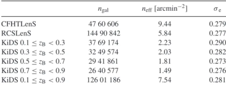
Table 1. Total number of galaxies with shape measurements,ngal, effective galaxy number density,neff, and ellipticity dispersionσefor CFHTLenS, RCSLenS and KiDS for the cuts employed in this analysis. We follow the prescription in Heymans et al. (2012) to calculateneffandσe.
ngal neff[arcmin−2] σ e
CFHTLenS 47 60 606 9.44 0.279
RCSLenS 144 90 842 5.84 0.277
KiDS 0.1≤zB<0.3 37 69 174 2.23 0.290 KiDS 0.3≤zB<0.5 32 49 574 2.03 0.282 KiDS 0.5≤zB<0.7 29 41 861 1.81 0.273 KiDS 0.7≤zB<0.9 26 40 577 1.49 0.276 KiDS 0.1≤zB<0.9 126 01 186 7.54 0.281
whereCκκ is the cosmic shear signal and σe2
neff is the shape noise term, withσ2
e being the dispersion per ellipticity component and
neffthe galaxy number density. These parameters are listed in
Ta-ble1. The cosmic shear termCκκ is calculated using the halo-model. The two terms in equation (16) are of similar magnitude, with the shape noise dominating at small scales and sampling variance dom-inating at large scales. Decreasingσe or increasingneffthus only
in this analysis, even though it is the deepest survey of the three. Although RCSLenS has the largest effective area, the covariance for KiDS is slightly smaller since the increase in depth is large enough to overcome the area advantage of RCSLenS.
4.2.2 Random patches
We select 100 random patches from the gamma-ray map as an approximation of independent realizations of the gamma-ray sky. The patches match the shape of the original gamma-ray cutouts, i.e. the lensing footprints plus a four degree wide band, but have their position and orientation randomized. The patches are chosen such that they do not lie within the Galactic latitude cut.
These random patches are uncorrelated with the lensing data but preserve the auto-correlation of the gamma rays and hence account for sampling variance in the gamma-ray sky, including residuals of the foreground subtraction.
For small patches, the assumption of independence is quite accu-rate, as the probability of two random patches overlapping is low. Larger patches will correlate to a certain degree. This lack of inde-pendence might lead to an underestimation of the covariance. This correlation is minimized by rotating each random patch, making the probability of having two very similar patches low.
The diagonal elements of the resulting covariance are shown in Fig.5. While the agreement with the Gaussian covariance is good at small scales, there is an excess of variance at large scales for some energy and redshift bins. This excess can be explained by a large-scale modulation of the power in the gamma-ray map, which would be sampled by the random patches. This interpretation is consistent with the strong growth of the error bars of the gamma-ray auto-correlation towards large scales. However, the results of the analysis are not affected significantly by this.
4.2.3 Randomized flux
In a further test of the analytical covariance in equation (13), we randomize the gamma-ray pixel positions within each patch. This preserves the one-point statistics of the flux while destroying any spatial correlations. This approach is similar to the random Poisson realizations used in Shirasaki et al. (2014) but we use the actual one-point distribution of the data itself instead of assuming a Poisson distribution.
Because the pixel values are not correlated anymore, contribu-tions to the large-scale variance due to imperfect foreground sub-traction or leakage of flux from point sources outside of their masks are removed.
The covariance derived from 100 such random flux maps is in good agreement with both the analytical covariance and the covari-ance estimated from random patches, as shown in Fig.5.
4.3 Statistical methods
The likelihood function we employ to find exclusion limits on the annihilation cross-section σannvor decay ratedecand WIMP
massmDMis given by
L(α|d)∝e−21χ2(d,α), (17)
with
χ2(d,α)=(d−μ(α))TC−1(d−μ(α)), (18)
whereddenotes the data vector,μ(α) the model vector,αthe pa-rameters considered in the fit, i.e. either the cross-sectionσannv
and the particle mass mDM or the decay rate dec and mDM.
The amplitude of the cross-correlation signal expected from as-trophysical sources is kept fixed and thus does not contribute as an extra free parameter. Finally, C−1 is the inverse of the
data covariance.
The limits on σannvand dec correspond to contours of the
likelihood surface described by equation (17). Specifically, for a given confidence intervalp, the contours are given by the set of parametersαcont.for which
χ2(d,α
cont.)=χ2(d,αML)+χ2(p), (19)
whereαMLis the maximum likelihood estimate of the parameters
σannvordecandmDM,χ2is given by equation (18), andχ2(p) corresponds to the quantile function of theχ2-distribution. For this
analysis we are dealing with two degrees of freedom and require 2σcontours, henceχ2(0.95)=6.18.
This approach to estimate the exclusion limits follows recent studies, such as Shirasaki et al. (2016). It should be noted that deriving the limits on σannvor dec for a fixed mass mDM is
also common in the literature [see e.g. Fornasa et al. (2016) for a recent example]. This corresponds to calculating the quantile functionχ2(p) for only one degree of freedom.
Care has to be taken when using data-based covariances, such as the random patches and randomized flux, as the inverse of these covariances is biased (Kaufman1967; Hartlap et al.2007). To account for the effect of a finite number of realizations, the Gaussian likelihood in equation (17) should be replaced by a modifiedt-distribution (Sellentin & Heavens2016). Alternatively, the effect of this bias on the uncertainties of inferred parameter can be approximately corrected (Hartlap et al. 2007; Taylor & Joachimi2014). In light of the large systematic uncertainties in this analysis we opt for the latter approach when using the data based covariances.
5 R E S U LT S
5.1 Cross-correlation measurements
We present the measurement of the cross-correlation of Fermi
gamma rays with CFHTLenS, RCSLenS and KiDS weak lensing data in Figs6–8, respectively. The measurements for CFHTLenS and RCSLenS use a single redshift bin and the five energy bins described in Section 3.2. The measurements for KiDS use the same energy bins but are further divided into the five redshift bins given in Section 3.1.3.
Besides the cross-correlation of the gamma rays and shear due to gravitational lensing (denoted by black circles), we also show the cross-correlation between gamma rays and the B mode of the shear as red squares. The B mode of the shear is obtained by rotating the galaxy orientations by 45◦, which destroys the gravitational lensing signal. Any significant B-mode signal would be indicative of spurious systematics in the lensing data.
Theχ2
0values of the measurements with respect to the hypothesis
of a null signal, i.e.μ=0, are listed in Table2. Theχ2
0 values are
Figure 6. Measurement of the cross-spectrum ˆCgκbetweenFermigamma rays and weak lensing data from CFHTLenS for five energy bins for gamma-ray photons (black points). The cross-spectrum of the gamma rays and CFHTLenS B modes are depicted as red data points.
Figure 7. Measurement of the cross-spectrum ˆCgκ betweenFermigamma rays and weak lensing data from RCSLenS for five energy bins for gamma-ray photons (black points). The cross-spectrum of the gamma rays and RCSLenS B modes are depicted as red data points.
with astrophysical sources,6the error bars would have to shrink by
a factor of 3 with respect to the current error bars for KiDS. This corresponds to an∼4000 deg2 survey with KiDS characteristics,
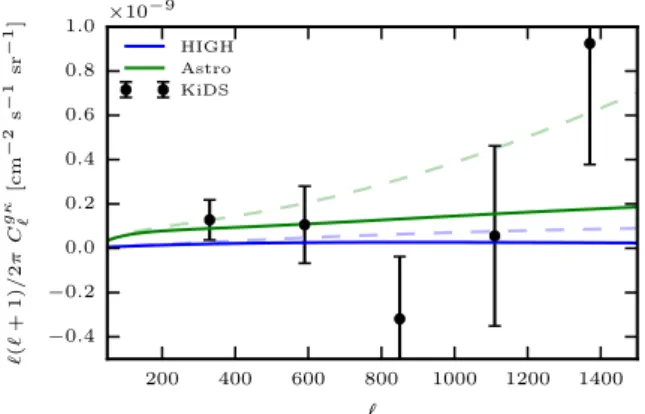
comparable in size to the galaxy surveys used in Xia et al. (2015). This is further illustrated in Fig.9, which shows the measurement for KiDS for the unbinned case in comparison with the expected correlation signal from astrophysical sources and annihilating dark matter for theHIGHscenario andσannv =3×10⁻²⁶cm3s−1for mDM=100 GeV and thebb¯channel. While these signals are not
ob-servable at current sensitivities, they are within reach of upcoming surveys, such as DES.7
The B-mode signal is consistent with zero for all measurements. We are thus confident that the measurement is not significantly contaminated by lensing systematics. At very small scales, lens-source clustering can cause a suppression of the lensing signal (van Uitert et al.2011; Hoekstra et al.2015). The angular scales we are probing in this analysis are, however, not affected by this.
5.2 Interpretation
We wish to exploit the measurements presented in the previous subsection to derive constraints on WIMP dark matter annihilation or decay. To derive the exclusion limits on the annihilation cross-sectionσannvand WIMP massmDM, and the decay ratedecand mDM, we apply the formalism described in Section 4.3.
In Camera et al. (2015) it was shown that the spectral and tomo-graphic information contained within the gamma-ray and lensing
6Cross-correlations between tracers of LSS and gamma rays have already been detected in Xia et al. (2015). A significant signal in the case of future weak lensing surveys is therefore a reasonable expectation.
7https://www.darkenergysurvey.org/
data can improve the limits onσannvanddec. We show the effect
of different combinations of spectral and tomographic binning for the case of KiDS and annihilations intobb¯ pairs under theHIGH
scenario in Fig.10and for dark matter decay in Fig.11. For these limits we adopt the conservative assumption that all gamma rays are sourced by dark matter, i.e. no astrophysical contributions are included. There is a significant improvement of the limits when using four energy bins over a single energy bin, especially at high particle massesmDM. This is due to the fact that the UGRB scales
roughly asE−2.3(Ackermann et al.2015c). The vast majority of the
photons in the 0.5–500 GeV bin therefore come from low energies. However, the peak in the prompt gamma-ray emission induced by dark matter occurs at energy∼mDM/20 (annihilating) or∼mDM/40
(decaying) forbb¯ and at higher energies for the other channels. Thus, for highmDM, a single energy bin of 0.5–500 GeV largely
in-creases the noise without significantly increasing the expected dark matter signal with respect to the 3.8–500 GeV bin.
The improvement due to tomographic binning is only marginal. Two factors contribute to this lack of improvement: first, in the case of no observed correlation signal – as is the case here – the differences in the redshift dependence of the astrophysical and dark matter sources do not come to bear because there is no signal to disentangle. Secondly, the lensing window functions are quite broad and thus insensitive to the featureless window function of the dark matter gamma-ray emissions, as depicted in Fig.1. This is due to the cumulative nature of lensing on the one hand and the fact that
photo-zs cause the truen(z) to be broader than the redshift cuts we impose on the other hand. This is in contrast with spectral binning, which allows us to sharply probe the characteristic gamma-ray spectrum induced by dark matter. As shown in Fig.3, annihilating dark matter shows a pronounced pion bump when annihilating into bb¯ and a cutoff corresponding to the dark matter mass mDM, while for
Figure 8. Measurement of the cross-spectrum ˆCgκbetweenFermigamma rays and weak lensing data from KiDS for five energy bins for gamma-ray photons and five redshift bins for KiDS galaxies (black points). The cross-spectrum of the gamma rays and KiDS B modes are depicted as red data points.
Table 2. χ2
0values with respect to the hypothesis of a null signal for the measurements of ˆC gκ
shown in Figs6–8. The number of degrees of freedom is the number of multipole bins, i.e.ν=5 for all measurements.
χ2 0
ˆ
Cgκ, ν=5
Energy bin [GeV] 0.5–0.8 0.8–1.4 1.4–3.8 3.8–500.0 0.5–500.0
CFHTLenS 4.49 7.77 3.78 8.43 2.43
RCSLenS 6.06 6.75 2.39 6.47 3.19
KiDS 0.1≤zB<0.3 5.96 1.85 6.53 6.89 8.47
KiDS 0.3≤zB<0.5 1.84 1.94 2.75 3.42 2.77
KiDS 0.5≤zB<0.7 3.27 1.89 4.02 2.56 5.57
KiDS 0.7≤zB<0.9 4.82 11.42 4.98 2.88 8.76
KiDS 0.1≤zB<0.9 7.16 1.81 5.42 3.05 6.55
mass. For this reason we refrain from a tomographic analysis for CFHTLenS and RCSLenS as we expect little to no improvements of the limits.
The limits can be further tightened by taking into account known astrophysical sources of gamma rays. This comes, however, at the expense of introducing new uncertainties in the modelling of said astrophysical sources. Going forward, we include the astrophysical sources to show the sensitivity reach of such analyses but also show the conservative limits derived under the assumption that all gamma rays are sourced by dark matter.
To account for the astrophysical sources, we subtract the combi-nation of the three populations (blazars, mAGN and SFG) described in Section 2 from the observed cross-correlation signal. The dark matter limits are then obtained by proceeding as before but using
the residuals between the cross-correlation measurement and the astrophysical contribution. Since we assume no error on the astro-physical models, the limits obtained by including blazars, mAGN and SFG contributions should be considered as a sensitivity reach for a future situation where gamma-ray emission from these astro-physical sources will be perfectly understood.
The resulting 2σ exclusion limits on the dark matter annihila-tion cross-secannihila-tion σannvfor thebb¯, μ−μ+ andτ−τ+ channels
Figure 9. Measurement of the cross-spectrum ˆCgκbetweenFermigamma rays in the energy range 0.5–500 GeV and KiDS weak lensing data in the redshift range 0.1–0.9 (black data points), compared to the expected signal from the sum of astrophysical sources (solid green) and annihilating dark matter (solid blue). The astrophysical sources considered are blazars, mAGN and SFG. The annihilating dark matter model assumes theHIGHscenario, mDM=100 GeV, andσannv =3×10⁻²⁶cm3s−1. The dashed lines show the same models but without correcting for theFermiPSF.
Figure 10. Exclusion limits on the annihilation cross-sectionσannvand WIMP massmDMfor the clustering scenariosHIGH(blue),MID(purple) and LOW(red) and for different binning strategies for the KiDS data. The lines correspond to 2σupper limits onσannvandmDM, assuming a 100 per cent branching ratio intobb¯. No binning in redshift or energy (1z x 1E) is denoted by dash–dotted lines. The case of binning in redshift but not energy (4z x 1E) is plotted as dotted lines, while binning in energy but not redshift (1z x 4E) is plotted as dashed lines. Finally, binning in both redshift and energy (4z x 4E) is shown as solid lines. The thermal relic cross-section, from Steigman, Dasgupta & Beacom (2012), is shown in grey.
Figure 11. Exclusion limits on the decay ratedecand WIMP massmDM for thebb¯channel for different binning strategies for the KiDS data. The style of the lines is analogous to Fig.10.
i.e. theHIGHmodel, and accounting for contributions from
astro-physical sources (dashed blue line), we can exclude the thermal relic cross-section for massesmDM20 GeV for thebb¯ channel.
In the case of annihilations or decays into muons or tau leptons, the exclusion limits change shape and become stronger for large dark matter masses, compared to thebchannel. This is due to the fact that, for heavy dark matter candidates, inverse Compton scattering produces a significant amount of gamma-ray emission in the upper energy range probed by our measurement (Ando & Ishiwata2016). If we make the conservative assumption that only dark matter con-tributes to the UGRB, i.e. we do not account for the astrophysical sources of gamma rays, the exclusion limits weaken slightly, as seen in the difference between the dashed and solid blue lines in Fig.13. In this case the thermal relic cross-section can be excluded formDM10 GeV for thebb¯channel. These limits are consistent
with those forecasted in Camera et al. (2015).
The exclusion limits when dark matter is assumed to be the only contributor to the UGRB are comparable to those derived from the energy spectrum of the UGRB in Ackermann et al. (2015a). However, when the contribution from astrophysical sources is ac-counted for, the limits in Ackermann et al. (2015a) improve by approximately one order of magnitude, while our limits see only modest improvements. This is due to the fact that we do not observe a cross-correlation signal. The constraining power therefore largely depends on the size of the error bars. The contribution from astro-physical sources is small compared to the size of our error bars, as shown in Fig.9, explaining the modest gain in constraining power when including the astrophysical sources compared to probes that observe a signal. The exclusion limits obtained in Fornasa et al. (2016) from the measurement of the UGRB angular auto-power spectrum are stronger than the ones presented here. Those lim-its are dominated by the emission from dark matter subhaloes in the Milky Way, a component that is not considered in our analy-sis since it does not correlate with weak lensing. When restricting the analysis of the auto-spectrum in Fornasa et al. (2016) to only the extragalactic components, our cross-correlation analysis yields more stringent limits. The limits presented here are comparable to those of similar analyses of the cross-correlation between gamma rays and weak lensing (Shirasaki et al. 2014, 2016) but weaker than those derived from cross-correlations between gamma rays and galaxy surveys (Cuoco et al. 2015; Regis et al. 2015). The exclusion limits from all these extragalactic probes are somewhat weaker than those derived from dSphs (Ackermann et al.2015b; Baring et al.2016).
Figure 12. Exclusion limits on the annihilation cross-sectionσannvand WIMP massmDMat 2σ significance for CFHTLenS, RCSLenS and KiDS and annihilation channelsbb¯,μ−μ+andτ−τ+. CFHTLenS and RCSLenS use four energy bins while KiDS additionally makes use of four redshift bins. The exclusion limits are for the three clustering scenariosHIGH(blue),MID(purple) andLOW(red). The dashed blue line indicates the improvement of the limits for theHIGHscenario when including the astrophysical sources in the analysis.
Figure 13. Exclusion limits on the annihilation cross-sectionσannvand WIMP massmDMat 2σsignificance for the combination of CFHTLenS, RCSLenS and KiDS. The style of the lines is the same as for Fig.12.
6 C O N C L U S I O N
We have measured the angular cross-power spectrum of Fermi
gamma rays and weak gravitational lensing data from CFHTLenS, RCSLenS and KiDS. Combined together, the three surveys span a total area of more than 1000 deg2. We made use of 8 years of Pass
8Fermidata in the energy range 0.5–500 GeV which was divided further into four energy bins. For CFHTLenS and RCSLenS, the measurement was done for a single-redshift bin, while the KiDS data were further split into five redshift bins, making this the first
measurement of tomographic weak lensing cross-correlation. We find no evidence of a cross-correlation signal in the multipole range 200≤ <1500, consistent with previous studies and forecasts based on the expected signal and current error bars.
Using these measurements we constrain the WIMP dark matter annihilation cross-sectionσannvand decay ratedecfor WIMP
Figure 14. Exclusion limits on the decay ratedecand WIMP massmDMat 2σsignificance for the combination of CFHTLenS, RCSLenS and KiDS (solid black). Including the astrophysical sources in the analysis results in the more stringent exclusion limits denoted by the black dashed line.
cross-section for WIMPs of masses up to∼20 GeV for thebb¯ chan-nel. Not accounting for the astrophysical contribution weakens the limits only slightly, while the exclusion limits for the more conser-vative clustering modelsMIDandLOWare a factor of∼10 weaker.
We find that tomography does not significantly improve the con-straints. However, exploiting the spectral information of the gamma rays strengthens the limits by up to a factor of∼3 at high masses.
The exclusion limits derived in this work are competitive with others derived from the UGBR, such as its intensity en-ergy spectrum (Ackermann et al. 2015a), auto-power spectrum (Fornasa et al.2016), cross-correlation with weak lensing (Shi-rasaki et al. 2014, 2016) or galaxy surveys (Regis et al. 2015; Cuoco et al.2015). Exclusion limits derived from local probes, such as dSphs, are stronger, however (Ackermann et al.2015b).
Future avenues to build upon this analysis include the use of up-coming large area lensing data sets, such as future KiDS data, DES, HSC,8LSST9and Euclid,10which will make it possible to detect a
cross-correlation signal between gamma rays and gravitational lens-ing. The analysis would also benefit from extending the range of the gamma-ray energies covered, by making use of measurements from atmospheric Cherenkov telescopes, which are more sensitive to high-energy photons (Ripken et al.2014).
Instead of treating the astrophysical contributions as a contami-nation to a dark matter signal, the measurements presented in this work could be used to investigate the astrophysical extragalactic gamma-ray populations that are thought to be responsible for the UGRB. We defer this to a future analysis.
AC K N OW L E D G E M E N T S
This work is based on observations obtained with MegaPrime/MegaCam, a joint project of CFHT and CEA/IRFU, at the CFHT which is operated by the National Research Council (NRC) of Canada, the Institut National des Sciences de l’Univers of the Centre National de la Recherche Scientifique (CNRS) of France, and the University of Hawaii. This research used the facilities of the Canadian Astronomy Data Centre operated by the National Research Council of Canada with the support of the Canadian Space Agency. CFHTLenS and RCSLenS data processing was made possible thanks to significant computing
8http://www.naoj.org/Projects/HSC/ 9http://www.lsst.org/
10http://sci.esa.int/euclid/
support from the NSERC Research Tools and Instruments grant programme.
This work is based on data products from observations made with ESO Telescopes at the La Silla Paranal Observatory under programme IDs 177.A-3016, 177.A-3017 and 177.A-3018, and on data products produced by Target/OmegaCEN, INAF-OACN, INAF-OAPD and the KiDS production team, on behalf of the KiDS consortium. OmegaCEN and the KiDS production team acknowl-edge support by NOVA and NWO-M grants. Members of INAF-OAPD and INAF-OACN also acknowledge the support from the Department of Physics & Astronomy of the University of Padova, and of the Department of Physics of Univ. Federico II (Naples).
Computations for theN-body simulations were performed in part on the Orcinus supercomputer at the WestGrid HPC consortium (www.westgrid.ca), in part on the GPC supercomputer at the SciNet HPC Consortium. SciNet is funded by: the Canada Foundation for Innovation under the auspices of Compute Canada; the Government of Ontario; Ontario Research Fund – Research Excellence; and the University of Toronto.
TT and LvW are funded by NSERC and CIfAR. TT is further-more supported by the Swiss National Science Foundation. SC is supported by ERC Starting Grant No. 280127. MF and SA ac-knowledge support from Netherlands Organization for Scientific Research (NWO) through a Vidi grant. MR and NF are supported by the research grant Theoretical Astroparticle Physics number 2012CPPYP7 under the programme PRIN 2012 funded by the Min-istero dell’Istruzione, Universit`a e della Ricerca (MIUR); by the research grants TAsP (Theoretical Astroparticle Physics) andFermi