THE ANALYTICAL AND EXPERIMENTAL MODELING
OF FUNCTIONING OF AUTOMATED INSTALLATIONS FROM CFF
CRISTIAN VASILE Faculty of Agronomy, University of Craiova, Romania
Keywords: automated control, experimental results, system equation, measurement ABSTRACT
The production of compound feed is very necessary for the nutrition of animals from livestock farms, both for the contribution of the good quality nutrients, and also for the reduction of animal products costs. For realizing the European Union’s rules regarding the processing of cereal products is necessary the endowing of all production capacities with modern and performance equipments, with high degree of mechanization, automation and computerization, with high productivities and with low specific consummations. Therefore it must be designed performing working installations whose functioning will be checked through experimental modeling so as to match the European rules.
INTRODUCTION
The analytical modeling is achieved for the most part in the designing phase of automation equipment, and the experimental is indicated to achieve for determining the correct functioning of the automation equipments which will be put into function. The experimental modeling take into account both the theoretical research of phenomena which conduct the analyzed action, and also the experimental research to confirm the theoretical hypotheses regarding the structure of those models and the determination of working parameters. The analytical models are useful when is determined the working structure or the installation’s compounds, they are not indicated for determining of parameters. The experimental modeling is translated into determination the optimal working model of the studied action through the processing of some experimental results.
This type of modelling consists in the following steps: a) planning and effectuating the experiment;
b) interpreting the experiment’s results;
c) determining the approximate model from the experimental data.[2]
The mathematical modelling which characterises the stationary point of an automated installation can be easily produced, usually due to an experiment. Experimental modelling is used for complex processes, when analytical modelling can determine only their form (structure), and the working parameters can be determined through a set of direct measurements. This article presents the determination of mathematical models (analytical) of the technological process of obtaining the compound feed by experimental data obtained during operation of the CFF installation work, meaning the values of input and output parameters measured during operation.[3, 4]
MATERIAL AND METHOD
Figure 1 presents a process with xi input and xe output („Single input - Single
output” type), considered as constantly working, meaning “no dead time” and which is affected by a xpdisturbance.
Figure 1 - The scheme of tehnological process
xp(t)
xi(t) xe(t)
Starting from the previous hypothesis, if we record the input values Xi(t) respectively output Xe(t) at the same time, we get a series of points in the plane (Xi,Xe). This means that for a input size value there are several output size values. The set of paired points (xi, xe ) form a correlation field.
= − ( , , , … , ) ≠ 0
= − ( , , , … , ) ≠ 0
...
= − ( , , , … , ) ≠ 0
In these types of mathematical modeling, it is highly recommended to use the method of the smallest squared values of the error when determining the parameters a0, a1,...,an from the condition clause which regards the sum of the squared differences in equations (1) that should be minimal:
∑ = ă
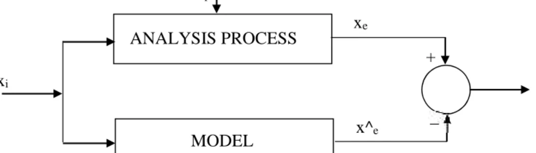
This method is the most commonly used in estimating the parameters of a model, determined by experimental data, because it is simple (figure 2) and offers a high degree of precision.
Figure 2: The scheme of the implementation of mathematical model
The one-dimensional linear regression method
This method consists of determining the parameters of a linear model with only one entry point and only one exit point, its form which could be expressed by the following equation:
= +
Due to the condition (1), the succession of values for the two types of parameters which have been registered in the same time are being concatenated, for this case the criteria function becoming:
( , ) = ∑ ( − ) = ∑ ( − − )
The values of the a0 and a1 parameters can be determined from the minimum condition of the criterion function. For this, we shall obtain an algebraic system consisting in two equations with variables of both sides (Cramer system), as shown below:
( , )= 0
( , )= 0
After operating these differential equations, we shall get the following final equation system:
ANALYSIS PROCESS
MODEL MATEM
xp
xi
xe
x^e
+
ε
(1) [1]
(2) [1]
(3) [1]
(4) [1]
In order to facilitate the calculation, the terms which contain unknowns will be replaced in the lelf-hand side and in the right-hand side those which don’t have unknowns, the system becoming:
+ (∑ ) = ∑
(∑ ) + (∑ ) = ∑
The expression vectors for the given system can write: ∑
∑ ∑ = ∑∑
Because of the simplicity of the system of equations (Crammer), the solution of the terms a0 and a1 is:
= (∑ )(∑(∑ ) (∑) ( ∑ )(∑) )
=(∑ ) − (∑ )(∑ )
(∑ ) − ( ∑ )
The multidimensional linear regression method
For the stationary technological processes with multiple sizes (figure 3), the mathematical model for the stationary may be determined by a multidimensional linear regression method. The mathematical model for such a system is described as:
= + + + ⋯ +
Figure 3: Input and output sizes that characterize a process
Also in this case we apply the method of the smallest error square. Considering that there is a number "M" of measurings of the direct parameters of technological proces, the criterial equation is:
( , , … , ) = ∑ [ − ] = ∑ [ − ( + + ⋯ + ] = ă
The minimum condition imposed in the criterial equation will generate a normal equations system like this:
( , ,…, ) = 0 ( , ,…, )
= 0 ...
( , , … , ) = 0 By solving differential equations, this system of equations becomes:
−2 ∑ [ − ( + + ⋯ + ] = 0
−2 ∑ [ − ( + + ⋯ + ] = 0
...
− 2 ∑ [ − ( + + ⋯ + ] = 0
(7) [1]
(8) [1]
(9) [1]
(10) [1]
(11) [1]
(12) [1] x1
x2
xn
ANALYSIS PROCESS xe
. . .
(13) [1]
Separating the amount components known and unknown to the left or to the right, the system of equations becomes:
M k ek ink M k ek k i M k ek n M k ink M k ink k i M k ik M k ink k i M k k i k i M k k i M k k i M k ink M k k i M k k ix
x
x
x
x
a
a
a
x
x
x
x
x
x
x
x
x
x
x
x
x
M
1 1 1 1 1 0 1 2 1 2 1 1 1 1 2 1 1 2 2 1 1 1 1 2 1 1)
(
)
(
It is noted that the system of normal equations has n + 1 equations with n + 1 unknowns, meaning is a compatible system of equations determined of type Crammer. The system 's solutions enable the complete determination of the multi-variable mathematical model formulated initially.
THE OBTAINED RESULTS
The final product resulted in the technological trial depends on several factors: a) the recipe used to produce this type of combined fodder;
b) the thermodynamic parameters of the steam generator.
On it's turn , the "factor" recipe is made, depending on the type of combined fodder, from 4 to 7 components, while the thermodynamic parameters of the steam generator are constant for each type of combined fodder, in number of 3. Analyzing these assumptions, the mathematical model that applies in this case is the methode of multidimensional linear regression.
During the technological process, were realized measurements of thermodynamic parameters and of the recipe. It was realized that the recipe component values were very accurate, the proportions being established directly from the raw material supplier, so the mathematical model will be easier, considering that the parameter recipe is a constant value. The only parameters that varied were the appropriate sizes to thermodynamic parameters and implicitly, of the finished product. The output size, meaning the finished product obtained, was analyzed qualitatively. It was considered that the finished product (combined fodder) is very good when the output value is 100.
Consequently the mathematical model consists of:
a) input data: temperature steam plant (Ta); temperature heat (Tat); pressure steam boiler (pa); constant recipe (Kr)
b) output data: finished product (Pf).
Further it presents the mathematical model of technological process, in which is producing compound feed type “Broiler chicken-starter phase”. The length of time measurement was about 100 minutes, and every 10 minutes was made the reading of parameters. Thus, each parameter which participate at the modelling of technological process of producing the combined feed analysed has 10 measured values (mean M=10). From literature of speciality, it is known that the modeling of technological processes through multidimensional linear regression method consists in solving a system of n + 1 equations with n + 1 unknowns, written in matrix form. At the elaboration of calcules has been used the software application Mathcad.
The values of the input parameters established for this mathematical model presents the following values, which is shown in table 1.
Table 1 The parameter values corresponding workflow
Parameter Value (j)
Kr 100 100 100 100 100 100 100 100 100 100
Ta 160 158 156 154 155 157 159 156 154 152
pa 7 6 5 6 4 5 6 4 5 9
Tat 190 188 186 184 182 185 180 188 187 192
Pf 100 99 98 96 95 94 93 92 97 93
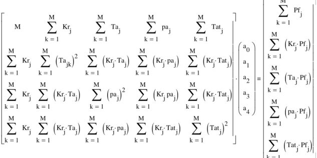
The mathematical model of automation process is described further by the following matrix equation:
To validate the model it is necessary to solve the symmetrically determined system of equations of Crammer’s type, in which its solutions a0, a1, a2, a3, a4must be values very
close to zero, and the differences between these must not be greater than 5%.
Thus, after calculations by using the measured values which were previously presented, the system solutions of equations has the following values:
1) a0= 0,00445
2) a1= 0,00563
3) a2= 0,00651
4) a3= 0,00523
5) a4= 0,00233
DISCUSSIONS
It is immediately observed that the values resulted before of the application of the mathematic model tend to the zero value, meaning the minimum value, so the mathematic value previously formed for the producing process of the compound feed is available.
Leaving from the same reasoning it can be said, for each situation individually, ie for a certain work installation or a certain type of combined fodder, every mathematic model concerning the automation of the production process.
The estimation of the parameters value of the linear models is being done with the help of the method of the smallest squares, in the normal equations systems.
From a mathematic point of view, the normal equation systems are, in fact, linear compatible determined algebraic systems, having symmetrical matrix.
M 1 M k Kr j
1 M k Kr j
1 M k Kr j
1 M k Kr j
1 M k Ta jk
2
1 M k KrjTaj
1 M k KrjTaj
1 M k Ta j
1 M k KrjTaj
1 M k pa j
2
1 M k Krjpaj
1 M k pa j
1 M k Krjpaj
1 M k Krjpaj
1 M k KrjTatj
1 M k Tat j
1 M k KrjTatj
1 M k KrjTatj
1 M k Tat j
2
a 0 a 1 a 2 a 3 a 4 1 M k Pf j
1 M k KrjPfj
1 M k TajPfj
1 M k pajPfj
1 M k TatjPfj
BIBLIOGRAPHY
1. Tănăsescu, N., 2000 – Modelarea matematică şi simularea numerică a proceselor
tehnologice din industria alimentară, Editura Matrix Rom, Bucureşti
2. Ţucu, D., 2007 – Sisteme tehnologice integrate pentru morărit şi panificaţie, Editura
Orizonturi Universitare, Timişoara
3. Vasile, C., 2010 – Studies on the Implementation of Automated Systems
to Prevent the Technical Problems Raised During the Production Process of Combined Fodders, Research Journal of Agricultural Science, vol 42 (nr. 1), pp. 663-670, ISSN: 2066-1843
4. Vasile, C., 2013 – Implementation of a Programmed Control System for the
Transportation of Raw Materials in a FNC, Annals of the University of Craiova – Agriculture, Montanology, Cadastre Series, Vol. XLIII, Vol.43, No.2, pages 241-247, ISSN: 1841-8317