Frequent Itemsets Patterns in Data Mining

(1)

Volume 1, Issue 6, August 2012

 Abstract

We are in the information age. In this age, we believe that information leads to power and success. The efficient database management systems have been very important assets for management of a large corpus of data and especially for effective and efficient retrieval of particular information from a large collection whenever needed. Unfortunately, these massive collections of data vary rapidly became overwhelming. Similarly, in data mining discovery of frequent occurring subset of items, called itemsets, is the core of many data mining methods. Most of the previous studies adopt Apriori –like algorithms, which iteratively generate candidate itemsets and check their occurrence frequencies in the database. These approaches suffer from serious cost of repeated passes over the analyzed database. To address this problem, we purpose two novel method; called Impression method, for reducing database activity of frequent item set discovery algorithms and Transaction Database Spin Algorithm for the efficient generation for large itemsets and effective reduction on transaction database size and compare it with the various existing algorithm. Proposed method requires fewer scans over the source database.

Keywords: Itemsets , Apriori , Database mining

INTRODUCTION

 Non-trivial extraction of implicit, previously unknown and potentially useful information from data warehouse

 Exploration & analysis, by automatic or semi-automatic means, of large quantities of data in order to discover meaningful patterns

 “Data mining is the entire process of applying computer-based methodology, including new techniques for knowledge discovery, from data warehouse.”

 A process that uses various techniques to discover “patterns” or knowledge from data.

Manuscript received Aug 3, 2012.

Leena Nanda, Computer Science, N.C.College of Engineering ,Isran , Panipat ,India,

Vikas Beniwal, Computer Science N.C.College of Engineering ,Israna, Gohana,India

 Look for hidden patterns and trends in data that is not immediately apparent from summarizing the data

Data mining, the extraction of hidden predictive information from large databases, is a powerful new technology with great potential to help companies focus on the most important information in their data warehouses. Data mining tools predict future trends and behaviors, allowing businesses to make proactive, knowledge-driven decisions. The automated, prospective analyses offered by data mining move beyond the analyses of past events provided by retrospective tools typical of decision support systems. Data mining tools can answer business questions that traditionally were too time consuming to resolve. They source databases for hidden patterns, finding predictive information that experts may miss because it lies outside their expectations.

Knowledge Discovery in Databases:

Data Mining, also popularly known as Knowledge Discovery in Databases (KDD), refers to the nontrivial extraction of implicit, previously unknown and potentially useful information from data in databases. The following figure (Figure 1.1) shows data mining as a step in an iterative knowledge discovery process. The Knowledge Discovery in Databases process comprises of a few steps leading from raw data collections to some form of new knowledge. The iterative process consists of the following steps:

•Data cleaning: also known as data cleansing, it is a phase in which noise data and irrelevant data are removed from the collection.

•Data integration: at this stage, multiple data sources, often heterogeneous, may be combined in a common source.

•Data selection: at this step, the data relevant to the analysis is decided on and retrieved from the data collection.

•Data transformation: also known as data consolidation, it is a phase in which the selected data is transformed into forms appropriate for the mining procedure.

•Data mining: it is the crucial step in which clever techniques are applied to extract patterns potentially useful.

Frequent Itemsets Patterns in Data Mining

(2)

Fig 1: Traditional process for Data Mining •Pattern evaluation: in this step, strictly interesting patterns representing knowledge are identified based on given measures.

•Knowledge representation: is the final phase in which the discovered knowledge is visually represented to the user. This essential step uses visualization techniques to help users understand and interpret the data mining results.

How does data mining work?

While large-scale information technology has been evolving separate transaction and analytical systems, data mining provides the link between the two and its software analyzes relationships and patterns in stored transaction data based on open-ended user queries. Types of analytical software are available: statistical, machine learning, and neural networks. Generally, any of four types of relationships are sought:

Classification: Stored data is used to locate data in predetermined groups. For example, a restaurant chain could mine customer purchase data to determine when customers visit and what they typically order. This information could be used to increase traffic by having daily specials.

Clusters: Data items are grouped according to logical relationships or consumer preferences. For example, data can be mined to identify market segments or consumer affinities.

Associations: Data can be mined to identify associations. The beer-diaper example is an example of associative mining.

Related Work:

Let I = {I1, I2… Im} be a set of m distinct attributes, also called literals. Let D be a database, where each record (tuple) T has a unique identifier, and contains a set of items such that T Є I An association rule is an implication of the form X=> Y, where X, YЄI, are sets of items called item sets, and X∩ Y=φ. Here, X is called antecedent, and Y consequent. Two important measures for association rules support (s) and confidence (α) can be defined as follows:

Support : The support (s) of an association rule is the ratio (in percent) of the records that contain X Y to the total

number of records in the database. For Example, if we say that the support of a rule is 5% then it means that 5% of the total records contain X  Y.

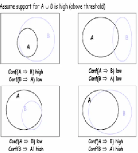
Confidence :For a given number of records, confidence (α) is the ratio (in percent) of the number of records that contain XY to the number of records that contain X. For Example, if we say that a rule has a confidence of 85%, it means that 85% of the records containing X also contain Y. The confidence of a rule indicates the degree of correlation in the dataset between X and Y. Confidence is a measure of a rule’s strength. Often a large confidence is required for association rules.[10]Different situations for support and confidence.

Fig 2.1 support and confidence situations

Basic Algorithm “APRIORI”: It is by far the most well known association rule algorithm. This technique uses the property that any subset of a large item set must be a large item set. The Apriori generates the candidate itemsets by joining the large itemsets of the previous pass and deleting those subsets, which are small in the previous pass without considering the transactions in the database. By only considering large itemsets of the previous pass, the number of candidate large itemsets is significantly reduced. In Apriori, in the first pass, the itemsets with only one item are counted. The discovered large itemsets of the first pass are used to generate the candidate sets of the second pass using the apriori_gen () function. Once the candidate itemsets are found, their supports are counted to discover the large itemsets of size two by scanning the database.. This iterative process terminates when no new large itemsets are found. Each pass i of the algorithm scans the database once and determine large itemsets of size i. Li denotes large itemsets of size i, while Ci is candidates of size i.

The apriori_gen () function has two steps. During the first step, L

(3)

apriori_gen () deletes all itemsets from the join result, which have x some (k-1)–subset that is not in L

K-1. Then, it returns

the remaining large k-itemsets. Consider the solve example in fig 2.3.

Method: apriori_gen ()

Input: set of all large (k-1)-itemsets L

K-1

Output: A superset of the set of all large k-itemsets //Join step Ii = Items i insert into C

K

Select p.I

1, p.I2, ……. , p.IK-1, q .IK-1

From L

K-1 is p, LK-1 is q

Where p.I

1 = q.I1 and …… and p.IK-2 = q.I K-2 and p.IK-1 <

q.I

K-1.

//pruning step for all itemsets c Є C

K

do for all (k-1)-subsets s of c do If (s∉L

K-1) then delete c from

C

K

The subset () function returns subsets of candidate sets that appear in a transaction. Counting support of candidates is a time-consuming step in the algorithm. Consider the below mentioned Algorithm.

Algorithm 1:

//procedure large Itemsets 1) C

1:=I; //Candidate 1-Itemsets

2) Generate L

1by traversing database and counting each

occurrence of an attribute in a transaction 3) for (K=2; L

k-1≠ϕ ;k++)

//Candidate itemsets generation

//New K-Candidate itemsets are generated from (k-1) large itemsets

4) Ck=apriori_gen (Lk-1) // counting support of Ck 5) Count (Ck, D)

6) Lk={C Є Ck | c.count ≥ minsup}

7) end 8) L: = υ k Lk

Apriori always outperforms AIS. Apriori incorporates buffer management to handle the fact that all the large itemsets L

K-1

and the candidate itemsets C

K need to be stored in the

candidate generation phase of a pass k may not fit in the memory. A similar problem may arise during the counting phase where storage for C

K and at least one page to buffer the

database transactions are needed.

Improving Apriori Algorithm Efficiency

• Transaction reduction –A transaction that does not contain any frequent k-item set is useless in subsequent scans.

• Partitioning –Any item set that is potentially frequent in Database must be frequent in at least one of the partitions of Database.

• Sampling – Mining on a subset of given data, lower support threshold + a method to determine the completeness.

Proposed Work Impression Algorithm:

These above approach suffer from serious cost of repeated passes over the analyzed database. To address this problem, we purpose a novel method; called Impression method, for reducing database activity of frequent item set discovery algorithms. The idea of this method consists of using Impression table for pruning candidate itemsets. The proposed method requires fewer scans over the source database. The first scan creates Impression, while the subsequent ones verify discovered itemsets.

The goodness of the Impression algorithm is: 1) Databases scans will be less,

2) Faster snip of the candidate itemsets.

Most of the previous studies on frequent itemsets adopt Apriori-like algorithms, which iteratively generate candidate itemsets and check their occurrence frequencies in the database. It has been shown that Apriori in its original form suffer from serious costs of repeated passes over the analyzed database and from the number of candidates that have to be checked, especially when the frequent itemsets to be discovered are long.

Impression method generates Impression table from the original database and use them for pruning candidate itemsets in the iteration.

Apriori-like algorithms use full database scans for pruning candidate itemsets, which are below the support threshold. Impression method prunes candidates by using dynamically generated Impression table thus reducing the number of database blocks read.

Impression Property:

A Impression table used by our method is a set of Impression generated for each database item set. The Impression of a set X is an N-bit binary number created, by means of bit-wise OR operation from the Impression of all data items contained in X.

The Impression has the following property. For any two set X and Y, we have X Є Y if:

Impr (X) AND Impr (Y) = Impr (X)

Where AND is the bit-wise AND operator. The property is not reversible in general (when we find that the above formula evaluates to TRUE we still have to verify the result traditionally).

Algorithm:

Scan D to generate Impression S and to find L

1;

For (K=2; L

K-1 ≠ 0; K++) do Begin

C

k = apriori_gen (Lk-1);

Begin

For all transactions t Є D do begin C

t = subset ( CK ,t);

For all candidate c Є C

t do c.count++;

(4)

End L

k = {c Є Ck | c.count ≥ minsup};

End Answer= υ

K L K;

Scan D to verify the answer;

Apriori_gen ()

The apriori_gen () function works in two steps:

1. Join step 2. Prune step

Transaction Database Snip Algorithm:

To determine large itemsets from a huge number of candidate large itemsets in early iterations is usually the dominating factor for the overall data mining performance. To address this issue we propose an effective algorithm for the candidate set generation. Explicitly, the number of candidate 2-itemsets generated by the proposed algorithm is, in order of magnitude, smaller than that by the previous method, thus resolving the performance bottleneck.

Another performance related issue is on the amount of data that has to be scanned during large item set discovery. Generation of smaller candidate sets by the snip method enables us to effectively trim the transaction database at much earlier stage of the iteration i.e. right after the generation of large 2-itemsets, therefore reducing the computational cost for later iteration significantly.

The algorithm proposed has two major features:

 Efficient generation for large itemsets.

 Reduction on transaction database size.

Here we add a number field with each database transaction. So when we check about the support of each item set in the candidate itemsets. Then if the candidate item set is the subset of that transaction then the number field is incremented by one each time.

After calculating the support of the candidate item set. Then we snip those transactions of the database that have: Number < length of the transaction.

So if the transaction is ABC then the number of this transaction should be 3 or greater than 3.i.e. at least 3 candidate itemsets are subset of this transaction.

So each time the database is sniped on these criteria. So input output cost is reduced, as the scanning time is reduced. Here we reduces the storage required by the candidate set item sets by only adding those itemsets in to the large itemsets which qualify the minimum support level.

Algorithm:

Scan D to generate Impression C1 and to find L1;

For (K=2; LK-1 ≠ 0; K++) do Begin

Ck = apriori_gen (Lk-1);

Begin

For all transactions t Є D do begin Ct = subset ( CK ,t);

For all candidate c Є Ct do c.count++; D.n++;

End

For all transactions t Є D do Begin If (n< transaction (length)) delete (database, transaction); End

End

Lk = {c Є Ck | c.count ≥ minsup};

End

Answer: υK L K;

RESULTS

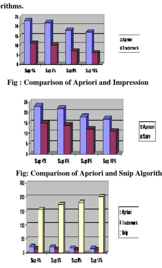
Graphical representation of the time taken by the various algorithms.

Fig : Comparison of Apriori and Impression

Fig: Comparison of Apriori and Snip Algorithm

Fig: Comparison of Apriori, Impression and Snip Algorithm The number of database scans:

-In the Apriori algorithm the number of database scan is of K times where K is the largest value of K in L

K or of CK.

-In the Impression method of number of database scans are only one i.e. while creating the signature table.

-In the Transaction Database Snip algorithm the number of database scans is of K times where K is the largest value of K in L

K or of CK. But the size of the database scanned is reduced

(5)

CONCLUSION

Performance study shows Impression method is efficient than the Apriori algorithm for mining in terms of time as it reduces the number of and Database scans, and also the Transaction Database Snip Algorithm is efficient than the Apriori algorithm for mining in terms of time, as it snip the database in each iteration. The Impression method is roughly two times faster than the Apriori algorithm, as Impression method does not require more than one database scan, and Transaction Database Snip Algorithm snip the database in each iteration.

REFERENCES

[1]Arun K Pujari. Data Mining Techniques (Edition 5): Hyderabad, India: Universities Press (India) Private Limited, 2003.

[2] Ashok Savasere ,Edward Omiecinski, Shamkant Navathe An Efficient Algorithm for mining Association rules in Large databases ,college of computing , Georgia Institute of technology, Atlanta.

[3] Bing Liu, Wynne Hsu and Yiming Ma, Integrating Classification and Association Rule Mining, American Association of Artificial Intelligence.

[4] Charu C. Aggarwal, and Philip S. Yu, A New Framework for Itemset Generation, Principles of Database Systems (PODS) 1998, Seattle, WA.

[5] Charu C. Aggarwal, Mining Large Itemsets for Association Rules, IBM research Lab.

[6] Gurjit Kaur in Data Mining: An Overview, Dept. of Computer Science & IT, Guru Nanak Dev Engineering College, Ludhiana, Punjab, India

[7] Jiawei Han. Data Mining, concepts and Techniques: San Francisco, CA: Morgan Kaufmann Publishers.,2004. [8] Jiawei Han and Yongjian Fu, Discovery of Multiple-Level Association Rules from Large Databases, Proceedings of the 21nd International Conference on Very Large Databases, pp. 420-431, Zurich, Swizerland, 1995 [9] Ja-HwungSu, Wen-Yang Lin CBW: An Efficient Algorithm for Frequent Itemset Mining, In Proceedings of the 37th Hawaii International Conference on System Sciences – 2004.

[10] Karl Wang: Introduction to Data Mining, Chapter-4, Conference in Hawaii.

[11]M. S. Chen, J. Han, and P. S. Yu. Data mining: An overview from a database perspective. IEEE Trans. Knowledge and Data Engineering, 1996.

[12] Marek Wojciechowski, An Hash – Mine algorithm for discovery of frequent itemsets , Maciej Zakrzewicz Institute of computer science, ul. Piotrowo 3a Poland.

[13]Ming Chen and Philip S. Yu An Effective Hash-Base Algorithm for Mining Association Rules. Jong Soo Park,, IBM Thomas J. Watson Research Center ,New York 1998

[14] Felman ,Ozel An Algorithm for Mining Association Rules, Using Perfect Hashing and Database Pruning in Proceedings of the 2007 in IEEE International Conference on Data Engineering .

Leena Nanda, M.Tech (Pursuing)