Numerical Solutions for Quadratic Integro Differential Equations of Fractional Orders

http://www.scirp.org/journal/ojapps ISSN Online: 2165-3925

ISSN Print: 2165-3917

Numerical Solutions for Quadratic

Integro-Differential Equations of Fractional

Orders

Fatheah Alhendi

1

, Wafa Shammakh

1

, Hind Al-Badrani

2 1_{Department of Mathematics, King Abdulaziz University, Jeddah, Saudi Arabia} 2_{Taibah University, Madinah, Saudi Arabia}

Abstract

In this article, variational iteration method (VIM) and homotopy perturbation method (HPM) solve the nonlinear initial value problems of first-order frac-tional quadratic integro-differential equations (FQIDEs). We use the Caputo sense in this article to describe the fractional derivatives. The solutions of the problems are derived by infinite convergent series, and the results show that both methods are most convenient and effective.

Keywords

Fractional Quadratic Integro-Differential Equations, Variational Iteration Method, Homotopy Perturbation Method

1. Introduction

The fractional calculus has appeared in many areas during the recent decades. Some scientists use approximation and numerical methods because there are almost no exact solutions of the fractional differential equations. He has pro- posed the VIM and HPM to solve the problems of linear and nonlinear [1] [2][3] [4]. VIM is based on Lagrange multiplier. The another method is HPM which defines as a coupling of the traditional perturbation method and homotopy in topology. Many authors successfully apply these methods to find the solutions of functional equations which arise in scientific and engineering problems [1] [5] [6] [7] [8] [9]. The Adomian decomposition method presents solution of functional equations but perhaps we find some difficulties that will arise during the computation of Adomian polynomials, the VIM and HPM overcome it is difficulties [7]. Fractional differential equations have diverse applications of physical phenomena [10] [11] [12] [13], for instance, acoustics, electromag- How to cite this paper: Alhendi, F.,

Shammakh, W. and Al-Badrani, H. (2017) Numerical Solutions for Quadratic Integro- Differential Equations of Fractional Or- ders. Open Journal of Applied Sciences, 7, 157-170.

https://doi.org/10.4236/ojapps.2017.74014

Received: March 5, 2017 Accepted: April 25, 2017 Published: April 30, 2017

Copyright © 2017 by authors and Scientific Research Publishing Inc. This work is licensed under the Creative Commons Attribution International License (CC BY 4.0).

http://creativecommons.org/licenses/by/4.0/

netism, control theory, robotics, viscoelastic materials, diffusion, edge detection, turbulence, signal processing, anomalous diffusion and fractured media [14]. In literature, Momani and Noor [15] used the Adomian decomposition method for solving the fourth order fractional integro-differential Equation. Elbeleze et al.

[16] [17], Kadem and Kilicman [18] applied the HPM and VIM methods for integro-differential Equation of fractional order with initial-boundary con- ditions. Recently, Gaafar [19] studied the existence and nondecreasing solution for the initial value problem of a quadratic integro-differential equations. How- ever, there is little work on nonlinear fractional quadratic integro-differential equations.

Our goal for this article is extending the analysis of VIM and HPM to construct the approximate solutions of the following nonlinear initial value problems for first-order fractional quadratic integro-differential equations.

( )

( )

( ) ( )

(

( )

)

0 0

y y , y d , 0 1,

x

k k

b Dα x g x λ x H x t F t t α

∞

=

= + < ≤

∑

∫

(1)

subject to the following initial condition:

( )

0

y 0 =

γ

, (2)

D

α is the fractional derivative in the caputo sense, F

(

y

( )

x

)

is any

nonlinear function, γ0 is real constant and g is given and can be approximated

by taylor polynomials.

2. Basic Definitions

In this section, we intend to present some basic definitions and properties of fractional calculus theory which are further used in this article.

Definition 1.

Areal function f x

( )

,x>0 is said to be in space Cµ,

µ ∈

R

if there exists

a real number p>µ, such that

( )

1

( )

p

f t =t f t , where f t₁

( )

∈C

(

0,∞

)

, and it

is said to be in the space n

C_µ if and only if fn∈C_µ, n∈N. Definition 2.

The Riemann-Liouville fractional integral operator of order α>0 of a function f ∈Cµ,µ≥ −1, is defined as

( )

_{( ) (}

)

1

( )

0 1

d , 0,

t

f t t sα f s s

α _α

α

−

= − >

Γ

∫

 (3)

( )

( )

0

.

f t = f t



Some properties of the operator _α _{can be found in [11], which are needed}

here, as follows:

for f ∈Cµ,µ≥ −1, ,α β ≥0 and

γ ≥ −

1

:

1.  α βf t

( )

=α β+ f t

( )

,

2.  α βf t

( )

= β αf t

( )

,

3.

₍

(

1

)

₎

.

1

t t

α γ γ α γ

α γ +

Γ +

=

Γ + +



( )

₍

_{) (}

)

1

( )

0 1 d , t m m

D f t t s f s s

m α α α − − = −

Γ −

∫

(4)

for 1 , , 0, 1

m m− < ≤

α

m m∈N t> f ∈C− .

Lemma 1.

If m− < ≤1

α

m m, ∈N f, ∈C_µm,

µ

≥ −1, the the following two properties

hold:

1. Dααf t

( )

= f t

( )

,

2.

(

)

( )

( )

1 ( )

( )

0 0 .

! k

m k

k

t

D f t f t f

k

α α −

=

= −

∑



3. Analysis of VIM

The basic concept of the VIM is constructing the correction functional for the fractional quadratic integro-differential equation sees Equation (1) with initial conditions,

( )

( )

( )

( )

( )

( ) ( )

(

( )

)

1 0 0

y y y

y , y d ,

k k k k

k

a

k k

x x x b D x g x

x H x s F s s

β _µ α

λ ∞ + =   = + _{ } −     −   

∑

∫

   (5)

( )

( )

_{( ) (}

)

( )

( )

( )

( ) (

)

(

( )

)

1 1 0 0 0 1

y y y

y , y d d ,

x

k k k k

k

a

k k

x x x s s b D s g s

s H s p F p p s

β _µ α

β λ ∞ − + =  = + − _ − Γ   − _ 

∑

∫

∫

  (6) β

 is the Rieman-Liouville fractional integral operator of order

1

m

β α

= + −

_, µ is a general Lagrange multiplier and y , k g s

( )

refers to the restricted variation (i.e.)

δ

yk =0,

δ

g s

( )

=0, to identify the approximate

Lagrange multiplier, construct the correctional function (6) which can be approximately expressed as:

( )

( )

( )

( )

( )

( ) ( )

(

( )

)

1 1 0 0 0 y y

y y , y d d ,

k k

x a

k k k k

k

x x

s b D s g s s H s p F p p s

µ λ + ∞ = =   +  − −  

∑



∫



∫

 (7)

taking the variation of Equation (7) to the independent variable yk we find

( )

( )

( )

1

( )

1

0 0

y y y d ,

x

k k k k

k

x x s b D s s

δ + δ δ µ ∞

=

 

= + _{ }



∑



∫

(8)

to make the previous equation stationary, we gain the following stationary conditions:

( )

( )

1 0, 0,

s x s x

s s

µ ₌ µ′ ₌

+ = = (9)

finally, the Lagrange multiplier is:

( )

s 1.

µ

= − ₍₁₀₎

( )

( )

_{( ) (}

)

( )

( )

( )

( ) (

)

(

( )

)

1 1 0 0 0 1

y y y

y , y d d ,

x

k k k k

k

a

k k

x x x s s b D s g s

s H s p F p p s

α _µ α

α λ ∞ − + =  = − − _ − Γ   − _ 

∑

∫

∫

(11)

( )

( )

( ) ( )

( ) ( )

(

( )

)

1 0 0

y y y y , y d ,

a

k k k k k k

k

x x α b Dα x g x

λ

s H x s F s s

∞ + =   = − _ − − _ 

∑

∫

  (12)

the initial approximation y0

( )

x can be selected by the following way which

satisfies initial conditions

( )

( )

0 0 0

y x =

γ

, where

γ

=y 0 . (13)

4. Analysis of HPM

The main concept of the HPM is constructing the homotopy for fractional quadratic integro-differential equation sees Equation (1),

(

)

( )

( ) ( )

( ) ( )

(

( )

)

0 0 0

1 y y y , y d 0,

a

k k

k k

p b Dα x p b Dα x g x

λ

x H s x F x x

∞ ∞

= =

 

− + _ − − _=

 

∑

∑

∫

(14)

( )

( )

( ) ( )

(

( )

)

0 0

y y , y d 0,

a

k k

b Dα x p g x

λ

x H s x F x x

∞ =

 

= _ + _=

 

∑

∫

(15)

[ ]

0,1

p∈ is an embedding parameter. If

p

=

0

, then Equation (15) turns into a linear Equation

( )

0

y 0,

k k

b Dα x

∞ =

=

∑

and when

p

=

1

, then Equation (15) becomes to be the original problem. The solution of Equation (1) can be considered as a power series in p which is the basic assumption of HPM :

( )

( )

( )

2

( )

3

( )

0 1 2 3

y x =y x +py x +p y x + p y x +, (16)

when

p

=

1

in (16) the approximate solution of Equation (1) can be as following

( )

0

( )

1

( )

2

( )

3

( )

y x =y x +y x +y x +y x +,

First, substitute the relation (16) in the Equation (15). Second, equate the terms which have the same power’s of p which yield to the following series of equations:

( )

0 0

: y 0,

p Dα x = (17)

( )

( )

( ) ( )

(

(

( )

)

)

1

1 0 1 0

0

: y y , y d ,

a

p Dα x =g x +λ x

∫

H s x F x x (18)

( )

( ) ( )

(

(

( )

)

)

( ) ( )

(

(

( )

)

)

2

2 0 2 1

0

1 1 0

0

: y y , y d ,

y , y d ,

a

a

p D x x H s x F x x

x H s x F x x

( )

( ) ( )

(

(

( )

)

)

( ) ( )

(

(

( )

)

)

( ) ( )

(

(

( )

)

)

3

3 0 3 2

0

1 2 1 2 1 0

0 0

: y y , y d

y , y d y , y d ,

a

a a

p D x x H s x F x x

x H s x F x x x H s x F x x

α _λ λ λ = + +

∫

∫

∫

(20)

and so on, the functions F F1, 2, satisfy the following condition:

( )

( )

( )

(

2

)

(

( )

)

(

( )

)

2

(

( )

)

0 1 2 1 0 2 1 3 2

y y y y y y

F x +p x +p x + =F x +pF x +p F x +

5. Applications

n this section, we apply VIM and HPM to first-order nonlinear (FQIDEs). Example 1.

Consider the following nonlinear first-order (FQIDEs):

( )

(

)

( ) ( )

0

y 1 e 3e y y d , 0 1,

x

x x

Dα x =x + + + x

∫

t t < ≤α (21)

subject to the following initial condition

( )

y 0 =1. (22)

According to VIM, the expression of the iteration formula (12) for Equation (21) can be observed in the following form:

( )

( )

( )

(

)

( ) ( )

1

0

y y y 1 e 3e y y d .

x

x x

k x k x D k x x k x k t t

α α

+

 

= − _ − + − − _



∫



 (23)

To avoid the difficulty of fractional integration, for the exponential term we take the truncated taylor expansion in (23), e.g., e ~ 1 2 3

2 6

x x x

x

+ + + _{to sa-}

tisfy the initial condition (22), we assume that the initial approximation has the following form y0

( )

x =1, first-order approximation takes the following form

by using iteration Formula (23):

( )

( )

( )

(

)

( ) ( )

(

)

(

)

(

)

1 0 0 0 0

0

2

y y y 1 e 3e y y d ,

3 6 5

1 ,

1 2 3

x

x x

x x D x x x t t

x x x

α α

α

α α α

 

= −  − + − − 

 

 ₋ 

= − _{Γ +} −_{Γ +} −_{Γ +} _

 

∫

 (24)

( )

₍

₎

₍

₎

₍

₎

(

)

(

)

(

)

(

)

(

(

)

)

(

)

₍

(

_{) (}

)

₎

(

)

₍

(

_{) (}

)

₎

(

)

(

) (

)

(

)

2 2 3 2 2 1

2 2 2 2

2 3

5 4 3 3 1

2

3 6 5

y 1

1 2 3

2

3 21 48 36

4 4 4 4 2 2

3

6 5 9 30 45

4 2 3

4

5 20

2 4 4

2 2

9 99 423 864 324 .

4 3 2

x x x x

x x x x α α α α α

α α α

α

α α

α α α α α

α

α α α α

α α

α α

α α

α

α α α α

α α + + + +  −  = − _ − − _

Γ + Γ + Γ +

 

 −  Γ +

−_ − − − _

Γ + Γ + Γ + Γ + Γ +

 

Γ +

− − − − − − −

Γ + Γ +

Γ +

− − −

Γ + Γ +

Γ +

+ + + + +

Γ + Γ +

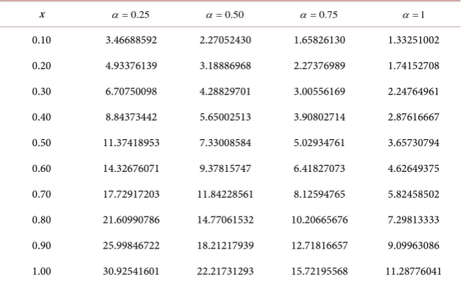
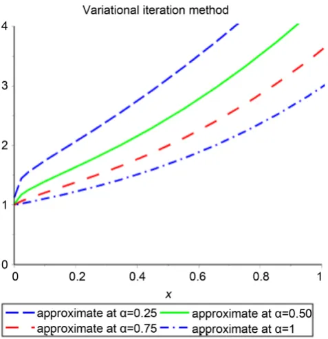
Table 1 and Figure 1 presents the approximate solution for the different values of α_{, we have noticed that the accuracy is improving. First, by computing} more terms of the approximate solutions. The second way is taking more terms in the taylor expansion of the exponential term.

According to HPM, we build the following homotopy:

( )

(

)

( ) ( )

0

y 1 e 3e y y d ,

x

x x

Dα x = p x_ + + + x t t_



∫

 (26)

First, substitute the relation (16) in the Equation (26).

[image:6.595.261.482.249.467.2]

Second, equate the terms which have the same power’s of p which yield to the following series of Equations:

[image:6.595.208.541.532.736.2]

Figure 1. Approximate solution for Equation (21) is ob- tained by VIM with different values of α_.

Table 1. Approximate solution for Equation (21) at different values of α_.

x α=0.25 α=0.50 α=0.75 α=1

( )

( )

(

)

( ) ( )

( )

( ) ( )

( ) ( )

0 1

0 1 0 0

0

2

2 0 1 1 0

0 0

: y 0, : y 1 e 3e y y d ,

: y y y d y y d ,

x

x x

x x

p D x p D x x x t t

p D x x t t x t t

α α α = = + + + = +

∫

∫

∫

(27)

and so on, apply the operator _α _{to the previous equations, and use the initial}

condition (22), to gain the following equations:

( )

0

y x =1, (28)

( )

(

)

( ) ( )

1 0 0

0

y 1 e 3e y y d ,

x

x x

x = α_x + + + x t t_



∫



 (29)

( )

( ) ( )

( ) ( )

2 0 1 1 0

0 0

y y y d y y d ,

x x

x = α_ x t t+ x t t_



∫

∫



 (30)

and so on, by taking the truncated taylor expansions for the exponential term in (29, 30): e.g., e ~ 1 2 3

2 6

x x x

x

+ + + to avoid the difficulty of fractional integra-

tion, thus by solving Equations (28, 29, 30), we obtain y , y ,1 2

( )

₍

₎

₍

1

₎

₍

2

₎

1

3 6 5

y ,

1 2 3

x x x

x

α α α

α α α

+ +

= + +

Γ + Γ + Γ + (31)

( )

(

₍

)

_{) (}

(

₎

)

(

₍

)

_{) (}

(

₎

)

(

)

(

)

(

) (

)

2 1 2 2

2

2 3

1 2 2 3

y 3 6

1 2 2 2 2 3

3 4

5 .

3 2 4

x x x

x

α α

α

α α α α

α α α α

α α

α α

+ +

+

Γ + + Γ +  Γ + + Γ + 

= _{Γ + Γ +} _ + _{Γ + Γ +} _

   

Γ + + Γ + 

+ _{Γ + Γ +} _

 

(32)

The two terms approximation are formed as the following Equation

( )

₍

₎

₍

₎

₍

₎

(

₍

)

_{) (}

(

₎

)

(

)

(

)

(

) (

)

(

(

)

) (

(

)

)

1 2 2 1 2

2 2 2 3

1 2

3 6 5

1 3

1 2 3 1 2 2

2 3 3 4

6 5

2 2 3 3 2 4

x x x

x x

x x

α α α

α

α α

α α

φ

α α α α α

α α α α

α α α α

+ +

+

+ +

Γ + + Γ + 

= + + + + _ _

Γ + Γ + Γ + _Γ + Γ + _

Γ + + Γ +  Γ + + Γ + 

+ _ _ + _ _

Γ + Γ + Γ + Γ +

   

(33)

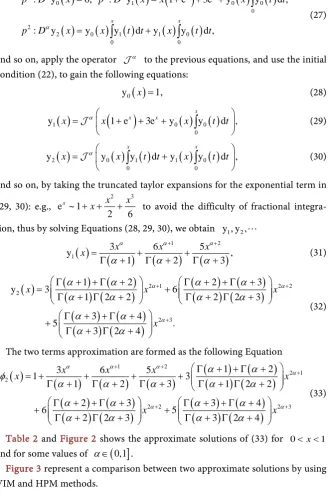
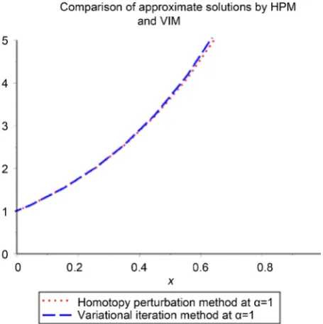
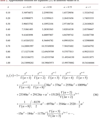
[image:7.595.211.545.87.582.2]

Table 2 and Figure 2 shows the approximate solutions of (33) for 0< <x 1 and for some values of α ∈

(

0,1

]

.

Figure 3 represent a comparison between two approximate solutions by using VIM and HPM methods.

Example 2.

Consider the following (FQIDEs):

( )

( )

2

( )

( )

0

y 1 y e y d , 0 1, y 0 1.

x t

Dα x = + x

∫

− t t < ≤α = (34)

According to VIM, the expression of the iteration Formula (12) for Equation (34) can be observed in the following form:

( )

( )

( )

( )

2

( )

1

0

y y y 1 y e y d .

x t

k x k x D k x k x k t t

α α −

+

 

= − _ − − _



∫



 (35)

[image:8.595.263.485.75.288.2]

Figure 2. Approximate solution for Equation (21) is obtained by HPM with different values of α_.

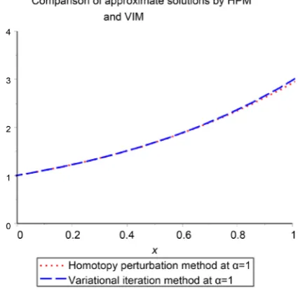
Figure 3. Comparison of approximate solution by using HPM and VIM at α=1.

take the truncated taylor expansion in (35), e.g., e ~ 1 2 3

2 6

x _{+ +x} x ₊x to satisfy the initial condition, we assume that the initial approximation has the following form y0

( )

x =1, first-order approximation takes the following form by using

iteration Formula (35):

( )

( )

( )

( )

( )

(

)

(

)

(

)

(

)

(

)

2

1 0 0 0 0

0

1 2 3 4

y y y 1 y e y d ,

1 ,

1 2 3 4 5

x t

x x D x x t t

x x x x x

α α

α α α α α

α α α α α

−

+ + + +

 

= − _ − − _

 

 − 

= −_ − + − + _

Γ + Γ + Γ + Γ + Γ +

 

∫

[image:8.595.263.491.332.561.2]

[image:9.595.211.541.76.470.2]

Table 2. Approximate solution for Equation (21) at different values of α_.

x α=0.25 α=0.50 α=0.75 α=1

0.10 3.34976072 2.25905581 1.65729056 1.33243542 0.20 4.53980075 3.12399413 2.26453456 1.74033333 0.30 5.90653782 4.10952104 2.97106726 2.24160625 0.40 7.51861405 5.28303363 3.82016538 2.85706667 0.50 9.41603098 6.68897807 4.84789742 3.61067708 0.60 11.63265252 8.36684782 6.09010254 4.52980000 0.70 14.20081997 10.35549050 7.58435402 5.64544792 0.80 17.15275198 12.69459789 9.37077013 6.99253333 0.90 20.52106372 15.42533768 11.49244150 8.61011875 1.00 24.33898202 18.59065973 13.99570082 10.54166666

( )

₍

₎

₍

₎

₍

₎

₍

₎

₍

₎

(

)

(

)

(

)

₍

(

)

₎

(

)

)

₍

(

)

₎

1 2 3 4

2

5

6 5 4 3

2 7 2 1

3 2 7

6 5 4 2 2

y 1

1 2 3 4 5

1

30 376 2550 10099

6 8

2

23340 29124 15120

2 2

1 8139 1

6970 3546 2520

8 2 2

3

15 184 1175

2 3

x x x x x

x

x

x

x

α α α α α

α

α

α

α α α α α

α α α α

α α

α

α α α

α

α α α α

α

α

α α α

α

+ + + +

+

+

+

= + + − + −

Γ + Γ + Γ + Γ + Γ +

+ + + + +

Γ + Γ +

Γ +

+ + + +

Γ +

− 

+ _ − − + −

Γ + 

Γ +

− − − +

Γ + ,

(36)

Table 3 and Figure 4 presents the approximate solution for the different values of α_{, we have noticed that the accuracy is improving. First, by computing} more terms of the approximate solutions. The second way is taking more terms in the taylor expansion of the exponential term.

According to HPM, we build the following homotopy:

( )

( )

2

( )

0

y 1 y e y d ,

x t

Dα x = p + x − t t



∫

 (37)

First, substitute the relation (16) in the Equation (37).

Second, equate the terms which have the same power’s of p which yield to the following series of Equations:

( )

( )

( )

( )

( )

( )

( ) ( )

( )

( )

0 1 2

0 1 0 0

0

2 2

2 0 0 1 1 0

0 0

: y 0, : y 1 y e y d ,

: y y e 2y y d y e y d ,

x t

x x

t t

p D x p D x x t t

p D x x t t t x t t

α α

α

−

− −

= = +

= +

∫

∫

∫

(38)

and so on, applying the operator _α _{to the previous Equations, and use the}

[image:9.595.206.542.90.476.2]

[image:10.595.257.496.74.321.2]

Figure 4. Approximate solution for Equation (34) is obtained by VIM with different values of α_.

Table 3. Approximate solution for Equation (34) at different values of α.

x α=0.25 α=0.50 α=0.75 α=1

0.10 1.74557818 1.39713379 1.20769182 1.10549607 0.20 2.06685872 1.63644354 1.37989631 1.22394067 0.30 2.39681774 1.88439871 1.56340949 1.35821602 0.40 2.74634447 2.15443603 1.76686736 1.51115026 0.50 3.11743203 2.45118250 1.99492282 1.68553370 0.60 3.51027500 2.77680334 2.25082546 1.88413224 0.70 3.92459385 3.13252560 2.53716249 2.10969920 0.80 4.35998072 3.51915865 2.85615873 2.36498657 0.90 4.81599699 3.93730820 3.20982456 2.65275652 1.00 5.29219083 4.38747370 3.60003936 2.97579365

( )

0

y x =1, (39)

( )

1

0

y 1 e d ,

x t

x = α_ + − t_



∫



 (40)

( )

( )

( )

2 1 1

0 0

y 2 e y d y e d ,

x x

t t

x = α_ − t t+ x − t_



∫

∫



 (41)

and so on, by taking the truncated taylor expansions for the exponential term in (40, 41): e.g., e ~ 1 2 3

2 6

x x x

x

− _{− + −}

.

[image:10.595.208.540.387.605.2]

( )

0

y x =1, (42)

( )

₍

₎

₍

1

₎

₍

2

₎

₍

3

₎

1

y ,

1 2 3 4

x x x x

x

α α α α

α α α α

+ + +

= + − +

Γ + Γ + Γ + Γ + (43)

( ) ( ) ( )

(

) (

₍

)

₎

_{( )}

₍

(

)

₎

(

) (

)

(

) (

₍

)

₎

_{( )}

₍

(

)

₎

( )

( )

(

(

)

)

5 4 3 2

2

2 1 2 1

5 4 3 2

2 2 2 2

2 2

2 1

y 1680 2 42 338 1302

7 6

2 1 2

2396

2 2 2 2

1

2 38 262 778

7 6

3 1 3

840

2 3 2 2 3

3 1

,

2 3

x

x x

x x

x

α α

α α

α

α α α α

α α

α α

α

α α α α

α α α α

α α

α α

α

α α α α

α α

α α α α

+ +

+ +

+

= + + + +

+ Γ +

Γ + Γ +

+ +

Γ + Γ Γ +

+ − − − −

+ Γ +

Γ + Γ +

− −

Γ + Γ Γ +

Γ +

+ +

Γ +

Γ + Γ 

(44)

the two terms approximation are formed as the following Equation

( )

₍

₎

₍

₎

₍

₎

₍

₎

(

) (

)

(

) (

₍

)

₎

_{( )}

₍

(

)

₎

1 2 3

2

5 4 3 2

2 1 2 1

1

1 2 3 4

1

1680 2 42 338 1302

7 6

2 1 2

2396 ,

2 2 2 2

x x x x

x

x x

α α α α

α α

φ

α α α α

α α α α

α α

α α

α

α α α α

+ + +

+ +

= + + − +

Γ + Γ + Γ + Γ +

+ + + + +

+ Γ +

Γ + Γ +

+ + +

Γ + Γ Γ + 

[image:11.595.237.539.73.282.2]

(45)

Table 4 and Figure 5 shows the approximate solutions of (34) for 0< <x 1 and for some values of α ∈

(

0,1

]

.

[image:11.595.217.544.76.513.2]

Figure 6 represent a comparison between two approximate solutions by using VIM and HPM methods.

[image:11.595.263.484.481.702.2]

[image:12.595.269.482.74.281.2]

Figure 6. Comparison of approximate solution by using HPM and VIM at α=1.

Table 4. Approximate solution for Equation (34) at different values of α_.

x α=0.25 α=0.50 α=0.75 α=1

0.10 1.74531342 1.39709144 1.20768552 1.10549521 0.20 2.06407267 1.63581216 1.37976305 1.22391477 0.30 2.38608229 1.88141089 1.56263514 1.35803058 0.40 2.71887729 2.14558172 1.76420974 1.51041158 0.50 3.06116974 2.43083965 1.98807470 1.68339534 0.60 3.40994267 2.73693555 2.23607620 1.87906377 0.70 3.76162440 3.06236426 2.50903647 2.09921280 0.80 4.11218308 3.40478991 2.80699405 2.34530601 0.90 4.45689697 3.76108758 3.12924403 2.61840230 1.00 4.78998433 4.12719346 3.47425744 2.91904762

Example 3.

Consider the following nonlinear (FQIDEs)

( )

( ) (

)

(

( )

)

( )

0

y 1 y ln y d , y 0 0.

x

x x x t t t

′ = +

_∫

− ′ = (46)

For x∈

[ ]

0,1 with exact solution y

( )

x =x. By using VIM, the iteration formula for Equation (46) is,

( )

( )

( )

( ) (

)

(

( )

)

1

0 0

y y y 1 y ln y d d .

x

n x n x n n r n r r

ζ

ζ

ζ

ζ

ζ

+

 

′ ′

= −  − − − 

 

∫

∫

(47)

We can take an initial approximation y0

( )

x =x.

The first two iterations are easily obtained from (47) and are given by:

( )

( )

( ) (

)

(

( )

)

1 0 0 0

0 0

y y 1 y ln y d d ,

x

x x r r r x

ζ

ζ

ζ

ζ

ζ

 _{′ ′} 

= − _ − − − _ =

 

[image:12.595.207.540.342.517.2]

( )

2

y x =x. (49)

Therefore, we obtain the exact solution, y

( )

x =x. According to HPM, we construct the following homotopy:

(

)

( )

( ) (

)

(

( )

)

0

, 1 ln d 0,

x

H u p =u x′ − −pu x

∫

x−t u t′ t= (50)

and continuously trace an implicity defined curve from starting point H u

( )

, 0

to a solution function H u

( )

,1 substituting (16) into (50). Also, we have to

equate the terms with the same identical power’s of p, then, we gain these components

( )

( )

0

0 0

: 1 ,

p u′ x = ⇒u x =x (51)

( )

( ) (

)

(

( )

)

( )

1

1 0 0 1

0

: ln d 0,

x

p u x′ =u′ x

∫

x−t u′ t t⇒u x = (52)

( )

( ) (

) ( )

1

_{( )}

( ) (

)

(

( )

)

2

2 0 1 0

0

0 0

: d ln d 0,

x _{u t} x

p u x u x x t t u x x t u t t

u t

′

′ = ′ − + ′ − ′ =

′

∫

∫

(53)

( )

( ) (

)

( )

_{( )}

( )

_{( )}

( ) (

)

( )

_{( )}

( ) (

)

(

( )

)

( )

2

2 1 1

3

3 0 2 1

0 0 0

0 0

2 0 3

0

1

: d d

2

ln d 0,

x x

x

u t u t u t

p u x u x x t t u x x t t

u t u t u t

u x x t u t t u x

 ′ ′   ′ 

′ = ′ − _{ ′} − _{′ } + ′ − _{ ′} _

 

 

′ ′

+ − ⇒ =

∫

∫

∫

(54)

and so on, we obtain u4=u5==0 therefore, the approximate solution is

obtained readily by y

( )

x n0un

( )

x u0

( )

x x ∞

=

=

∑

= = _{which is the exact solution.}

6. Conclusion

In this paper, we have applied the VIM and HPM to find the solution of nonlinear initial value problem of fractional quadratic integro-differential equations for the first order. The methods do not require any linearization, perturbation or restrictive assumptions, we have observed that the VIM and HPM is a very powerful and effective tool for finding the solutions of the fractional quadratic integro-differential Equation. We use the Maple package (2015) in calculations.

References

[1] He, J.H. (1999) Homotopy Perturbation Technique. Computer Methods in Applied Mechanics and Engineering, 178, 257-262.

[2] He, J.H. (1999) Variational Iteration Method—A Kind of Non-Linear Analytical Technique: Some Examples. International Journal of Non-Linear Mechanics, 34, 699-708.

[3] He, J.H. (2000) A Coupling Method of a Homotopy Technique and a Perturbation Technique for Non-Linear Problems. International Journal of Non-Linear Mechan-ics, 35, 37-43.

[4] He, J.H. (2003) Homotopy Perturbation Method: A New Nonlinear Analytical Technique. Applied Mathematics and Computation, 135, 73-79.

Riemann-Liouville’s Fractional Derivatives by He’s Variational Iteration Method. Journal of Computational and Applied Mathematics, 207, 53-58.

[6] Daftardar-Gejji, V. and Jafari, H. (2007) Solving a Multi-Order Fractional Differen-tial Equation Using Adomian Decomposition. Applied Mathematics and Computa-tion, 189, 541-548.

[7] Odibat, Z. and Momani, S. (2009) The Variational Iteration Method: An Efficient Scheme for Handling Fractional Partial Differential Equations in Fluid Mechanics. Computers & Mathematics with Applications, 58, 2199-2208.

[8] Sweilam, N.H. (2007) Fourth Order Integro-Differential Equations Using Varia-tional Iteration Method. Computers & Mathematics with Applications, 54, 1086- 1091.

[9] Yıldırım, A. (2008) Solution of BVPs for Fourth-Order Integro-Differential Equa-tions by Using Homotopy Perturbation Method. Computers & Mathematics with Applications, 56, 3175-3180.

[10] Benson, D.A., Wheatcraft, S.W. and Meerschaert, M.M. (2000) Application of a Fractional Advection-Dispersion Equation. Water Resources Research, 36, 1403- 1412. https://doi.org/10.1029/2000WR900031

[11] Miller, K.S. and Ross, B. (1993) An Introduction to the Fractional Calculus and Fractional Differential Equations.Wiley-Interscience, Hoboken.

[12] Podlubny, I. (1998) Fractional Differential Equations: An Introduction to Fractional Derivatives, Fractional Differential Equations, to Methods of Their Solution and Some of Their Applications. Academic Press, Cambridge, MA.

[13] Podlubny, I. (2002) Correction to Figure 4 in Geometric and Physical Interpretation of Fractional Integration and Fractional Differentiation. Fractional Calculus & Ap-plied Analysis, 5, 367-386.

[14] Nawaz, Y. (2011) Variational Iteration Method and Homotopy Perturbation Me-thod for Fourth-Order Fractional Integro-Differential Equations. Computers & Mathematics with Applications, 61, 2330-2341.

[15] Momani, S. and Noor, M.A. (2006) Numerical Methods for Fourth-Order Fraction-al Integro-DifferentiFraction-al Equations. Applied Mathematics and Computation, 182, 754-760.

[16] Elbeleze, A.A., Kilicman, A. and Taib, B.M. (2012) Application of Homotopy Per-turbation and Variational Iteration Methods for Fredholm Integrodifferential Equa-tion of FracEqua-tional Order. Abstract and Applied Analysis, 2012, Article ID: 763139. [17] Elbeleze, A.A., Kilicman, A. and Taib, B.M. (2016) Approximate Solution of

Inte-gro-Differential Equation of Fractional (Arbitrary) Order. Journal of King Saud University-Science, 28, 61-68.

[18] Kadem, A. and Kilicman, A. (2012) The Approximate Solution of Fractional Fred-holm Integrodifferential Equations by Variational Iteration and Homotopy Pertur-bation Methods. Abstract and Applied Analysis, 2012, Article ID: 486193. https://doi.org/10.1155/2012/486193

Submit or recommend next manuscript to SCIRP and we will provide best service for you:

Accepting pre-submission inquiries through Email, Facebook, LinkedIn, Twitter, etc. A wide selection of journals (inclusive of 9 subjects, more than 200 journals)

Providing 24-hour high-quality service User-friendly online submission system Fair and swift peer-review system

Efficient typesetting and proofreading procedure

Display of the result of downloads and visits, as well as the number of cited articles Maximum dissemination of your research work

Submit your manuscript at: http://papersubmission.scirp.org/