Oviedo University Press
Modelling and trading commodities with a new deep belief network
Andreas Karathanasopoulos*
University of Dubai, Dubai
Received: 4 August 2016
Revised: 1 May 2017
Accepted: 18 May 2017
Abstract
The scope of this project is to study a novel methodology in the task of forecasting and trading the crack spread modelled index. More specifically in this research we are expanding the earlier work carried out by Karathanasopoulos et al. (2016c) and Dunis et al. (2005) who model the Crack Spread with traditional neural networks. In this research paper we provide for first time a more advanced approach to non-linear mode
period covers 4500 trading days and the proposed model is a deep belief network (DBN). To model, test and evaluate the crack spread we use an expansive universe of 500 inputs correlated with the main index. Moreover we have used for reasons of comparison a radial basis function combined with partial swarm optimizer and two linear models such as random walk theorem and buy and hold strategy.
Keywords: spread trading; deep belief networks; PSO RBF neural networks
JEL Classification Codes: Q02, C15, C53
1. Introduction
In this paper, we propose a deep belief network DBN for short-term prediction of the crack
is the first time that deep beliefs networks have been used in the area of oil predictions. Secondly it is first time that 500 inputs have been used for the training of deep beliefs networks. The basic idea behind this analysis is to apply 3 different oil commodities in the equation 1 and try to predict one day ahead the Crack Spread. All the three commodities under our research are crude oil, gasoline and heating oil and all of them are traded in the New York Mercantile Exchange
* E-mail: [email protected].
(NYMEX).After running both artificial intelligent models we reveal that neural networks offer interesting results and seems that outperform the traditional linear models.
previously mentioned we are using three commodity variables. The input variable is the crude oil (CL) which is denominated in US dollars per barrel while the outputs consist of gasoline (RBOB) and heating oil (HO) which both are denominated in US cents per gallon. In terms of creating the equation and applying our three variables we need to convert them in the same units. Because the quantity of a crude oil contract is coming in 1,000 barrels per contract and both the gasoline and heating oil amount are coming to 42,000 gallons per contract, the latter two needs to be multiplied by 0.42. After these adjustments the equation is taking the below form. 3 )) CL x (3 -0.42)) x HO x (1 + 0.42) x RBOB x (((2 = St SPREAD CRACK 1 : 2 : 3 (1)
The final form of equation 1 is the below where we are converting the variables of daily prices to returns. Butterworth and Holmes (2002), Dunis et al. (2006) and Karathanasopoulos et al. (2016b) have used the same way to forecast the crack spread.
) (
) (
)
( ( 1)
) 1 ( ) ( ) 1 ( ) 1 ( ) ( ) 1 ( ) 1 ( ) ( t CL t CL t CL t HO t HO t HO t RBOB t RBOB t RBOB t P P P P P P P P P S (2)
2. Literature review
3. Data
As we have described in the first part, in the prediction of the crack spread we will use three different future contracts such as Crude oil (WTI), Unleaded Gasoline (RBOB) and Heating oil. In terms of training both neural networks we will divide the data set into training and validation sub sets. Below we are presenting how we are dividing the whole data set. In terms of optimizing the data set we used around 100 different data combinations. The one presenting in the table 1 is the only one that gives the best performance for both nonlinear models.
Table 1. Dataset
Name of Period trading days Number of Beginning End
Full Sample 4500 1/1/2000 31/12/2016
Training Period 3200 1/1/2000 1/1/2011
Validation Period 1300 2/1/2012 31/12/2016
4. Trading signals and strategy
Trading signals are generated based on directional forecasts of commodity prices. When a model forecasts a negative return, then a short position (sale) is assumed at the close of each day and when the model forecasts a positive return a long position (purchase) is executed. Profits and losses are computed using daily data.
5. Forecasting models
5.1. Random walk model
The first benchmark we employ is the random walk forecast of log crude oil prices. The random walk model is a widely used benchmark in the crude oil prediction literature, Bauimester and Kilian (2012), Alquist et al. (2013) and Karathanasopoulos et al. (2014). Let Yt denote the log
price of oil on day t.
,
1 t
t Y
Y (3)
where Yt 1 is the predicted log oil price on day t+1. Consistent with the existing literature, we start by evaluating the predictive and trading performance of the random walk model.
5.2. Buy-and-hold strategy
This simple strategy assumes that the investor opens a long position and keep the position open till the moment his investment grows, instead of selling it.
5.3. Radial basis functions - Particle swarm optimization
function and have an initial fitness price. Each particle flies through the problem space with a specific velocity that directs the flying. The aim of all particles is to find the optimal solution. This is achieved through a number of iterations. The maximum number of iterations is 350 and on average the optimal solution is coming after 100 iterations.
5.4. Deep beliefs networks
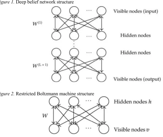
Deep belief network is a new probabilistic feed-forward forecasting tool with input layer and output layer (see figure 1).
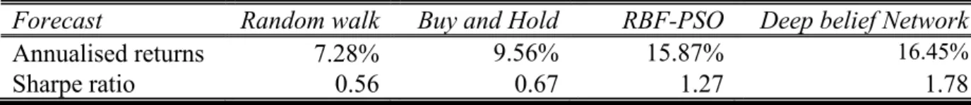
The basic idea behind this new model is the use a layer by-layer unsupervised learning method in order to pre-train the initial values of the weights in the neural network. A layer-by-layer unsupervised training procedure implies that each layer-by-layer captures the features of the previous one, and transferring them to next one. In this research paper each pair of layers is pre trained by using the restricted Boltzmann machines. Restricted Boltzmann machines are composed from 2 different layers connected together. One layer has visible nodes/neurons and the other hidden nodes/neurons (see figure 2).
Figure 1. Deep belief network structure
Figure 2. Restricted Boltzmann machine structure
The nodes on each layer have no connections between them only with units of other layers. All these connections are symmetric and bidirectional. As i mentioned before the restricted Boltzmann machines have been used in a numerous tasks but in our experiment are providing the learning training for the structure of the deep belief network. In few words restricted Boltzmann machines are a special type of generative energy based models that can learn a probability distribution over its set of inputs. Further to that the standard type of restricted Boltzmann machine has binary valued hidden and visible nodes.
In the below equation vi and hj represent the states of visible node i and hidden node j. For
i i ij j
j
hj p h v b w v
p 1 (4)
where (·) is the logistic sigmoid function, bj is the bias of j, i is the binary state, wij is the
weight between iand hj.
probability:
j j ij i
i
vi pv h b w h
p 1 (5)
In terms of training the network firstly a training sample is presented to the visible nodes, and the { i} is obtained. Then the hidden nodes state that {hj} are sampled according to
proba-bilities in equation 4. This process is repeated till the moment we will update the visible and then the hidden nodes, and the developed states i and hj are obtained. Hence the weights are
coming in the below form:
j i j i
ij vh v h
w ' ' (6)
where is the learning rate, and <·> refers to the expectation of the training data.
The continuous restricted Boltzmann has been built from Chao et al. (2011) and Chen and Murray (2002) where the inputs nodes are represented as si, and the output nodes as sj:
1 , 0
j i
i ij j
j w s
s (7)
where j(x) is a sigmoid function, Nj(0, 1) represents a Gaussian unit, is a constant, and ajis
a - e slope of the sigmoid function.
Instead of building the DBN we are using as many RBMs as the number of hidden layers In order to run the DBN model to forecast the Crack spread forecast we are using two hidden layers. Finally, in terms of constructing the DBN we will use the backpropagation learning algorithm in terms of getting better optimal outputs.
6. Empirical results
In tables 2 and 3 we are presenting the statistical and empirical performance in the out-of-sam-ple period for all the models. The measures we used are the Mean Absolute Error (MAE), the mean absolute percentage error (MAPE) the Root Mean Squared Error (RMSE), the annualized returns and the Sharpe ratio.
In this section we present the results of the proposed methodologies applied to the crack spread in the relevant out-of-sample period. The trading rule that we follow is simple. We go or stay long when the forecasted returns are above zero and go or stay short when the forecasted returns are below zero.
After taking consideration the above results its straightforward that the new feed forward deep belief network outperforms the RBF-PSO and the other two linear models. In the mean-time, these findings are not coming from a single run of the models but from the average of 100
Table 2. Out of sample statistical performance for Crack Spread
Forecast Random walk Buy and Hold RBF-PSO Deep belief Network
MAE 0.0230 0.0205 0.0190 0.0134
MAPE 209.66% 200.30% 190.33% 183.44%
RMSE 0.0190 0.0179 0.0167 0.0125
Table 3. Out of sample trading performance results for Crack Spread (including cost)
Forecast Random walk Buy and Hold RBF-PSO Deep belief Network
Annualised returns 7.28% 9.56% 15.87% 16.45%
Sharpe ratio 0.56 0.67 1.27 1.78
7. Concluding remarks
In this research paper, we propose a deep belief network DBN for oil predictions. More specif-ically the forecasting deep belief network is used to forecast the crack spread modelled index. Its first time in the whole literature that such model has been used in the area of data series
series. The evaluation of the forecasted returns has been measured through statistical and em-pirical analysis. After benchmarking the new methodology with a random walk model, a buy and hold strategy and a radial basis functions model combined with partial swarm optimizer we are coming to a clear result that DBNs are performing successfully in the real world and seem to be a huge challenging tool for managers and traders.
References
Alquist, R., Kilian, L. And Vigfusson, R.J. (2013) Forecasting the Price of Oil, Handbook of Economic Forecasting, Elsevier.
Baumeister, C. and Kilian, L. (2012) Real-Time Analysis of Oil Price Risks Using Forecast Scenarios, Staff Working Papers, 12, 1, Bank of Canada.
Butterworth, D. and Holmes, P. (2002) Inter-Market Spread Trading: Evidence from UK Index Futures Markets, Applied Financial Economics, 12(11), 783-791.
Chao, J., Shen, F. and Zhao, J. (2011) Forecasting exchange rate with deep belief networks, in
Proceedings of the International Joint Conference on Neural Networks ,
1259 1266, San Jose, Calif, USA,
Chen, H. and Murray, A.F. (2002) A continuous restricted Boltzmann machine with hardware-amenable learning algorithm, Proceedings of the 12th International Conference on Artificial Neural Networks, 358 363.
Ding, H., Xiao, Y. and Yue, J. (2005) Adaptive Training of Radial Basis Function Networks Using Particle Swarm Optimization Algorithm, Lecture Notes in Computer Science, 3610, 119- 128.
Dunis, C.L., Laws, J. and Evans, B. (2005) Modelling and Trading The Gasoline Crack Spread: A Non-Linear Story, Derivatives Use, Trading & Regulation, 12 (1-2), 126-145. Dunis, C.L, Laws, J. And Evans, B. (2006) Modelling and Trading the Soybean-Oil Crush
Hinton, G.E. and Salakhutdinov, R.R. (2006) Reducing the dimensionality of data with neural networks, Science, 313(5786), 504 507.
Hinton, G.E., Osindero, S. and Teh, Y.W. (2006) A fast learning algorithm for deep belief nets,
Neural Computation, 18(7), 1527 1554,
Kang, Y. And Choi, S. (2011) Restricted deep belief networks for multi-view learning, Lecture Notes in Computer Science, 6912, 130 145.
Karathanasopoulos, A., Dunis, C. and Khalil, S. (2016a) Modelling, forecasting and trading with a new sliding window approach: the crack spread example, Quantitative Finance, 16(12), 1875-1886.
Karathanasopoulos, A., Dunis, C., Likothanassis, S., Sermpinis, G. and Theofilatos, K. (2013) A Hybrid Genetic Algorithm-Support Vector Machine Approach in the Task of Forecasting and Trading, Journal of Asset Management, 14, 52-71.
Karathanasopoulos, A., Mitra, S., Skindilias, K. and Lo, C.C. (2016b) Modelling and Trading the English and German Stock Markets with Novelty Optimization Techniques, Journal of Forecasting, in press.
Karathanasopoulos, A., Sermpinis, G., Laws, J. and Dunis, C. (2014) Modelling and Trading the Greek Stock Market with Gene Expression and Genetic Programing Algorithms,
Journal of Forecasting, 33(8), 596-610.
Karathanasopoulos, A., Sermpinis, G., Stasinakis, C. and Theofilatos, K. (2015) Forecasting US Unemployment with Radial Basis Neural Networks, Kalman Filters and Support Vector Regressions, Computational Economics, 1-19.
Karathanasopoulos, A. (2016c) Modelling and trading the English stock market with novelty optimization techniques, Economics and Business Letters, 5(2), 50-57.
Kennedy, J. and Eberhart, R. (1995) Particle Swarm Optimization, Proceedings of the IEEE International Conference on Neural Networks, 4, 1942-1948.
Lee, H., Grosse, R., Ranganath, R. and Ng, A.Y. (2009) Convolutional deep belief networks for scalable unsupervised learning of hierarchical representations, Proceedings of the 26th International Conference On Machine Learning, 609 616.
Liu, T. (2010) A novel text classification approach based on deep belief network, Lecture Notes in Computer Science, 6443, 314 321,
Nekoukar, V. and Beheshti, H. (2010) A Local Linear Radial Basis Function Neural Network for Financial Time-Series Forecasting, Applied Intelligence, 33(3), 352-356.
Sermpinis, G., Theofilatos, K., Karathanasopoulos, A., Georgopoulos, E. and Dunis, C. (2013) Forecasting Foreign Exchange Rates with Adaptive Neural Networks Using Radial-Basis Functions and Particle Swarm Optimization, European Journal of Operational Research, 225(3), 528-540.
Shen, W., Guo, X., Wu, C. and Wu, D. (2011) Forecasting Stock Indices Using Radial Basis Function Neural Networks Optimized by Artificial Fish Swarm Algorithm, Knowledge-Based Systems, 24(3), 378-385.
Zhou, S., Chen, Q. and Wang, X. (2010) Discriminative Deep Belief networks for image classification, Proceedings of the 17th IEEE International Conference on Image