A Practical Incremental Learning Framework For Sparse Entity Extraction

Proceedings of the 27th International Conference on Computational Linguistics, pages 700–710 700

A Practical Incremental Learning Framework

For Sparse Entity Extraction

Hussein S. Al-Olimat1∗, Steven Gustafson2, Jason Mackay3 Krishnaprasad Thirunarayan1, and Amit Sheth1 1_{Kno.e.sis Center, Wright State University, Dayton, OH}

{hussein;tkprasad;amit}@knoesis.org

2_{Maana Inc, Bellevue, WA}

[email protected]

3 _{GoDaddy Inc, Kirkland, WA}

[email protected]

Abstract

This work addresses challenges arising from extracting entities from textual data, including the high cost of data annotation, model accuracy, selecting appropriate evaluation criteria, and the overall quality of annotation. We present a framework that integrates Entity Set Expansion (ESE) and Active Learning (AL) to reduce the annotation cost of sparse data and provide an online evaluation method as feedback. This incremental and interactive learning framework allows for rapid annotation and subsequent extraction of sparse data while maintaining high accuracy.

We evaluate our framework on three publicly available datasets and show that it drastically re-duces the cost of sparse entity annotation by an average of85%and45%to reach0.9and1.0 F-Scores respectively. Moreover, the method exhibited robust performance across all datasets.

1 Introduction

Entity extraction methods delimit all mentions of an entity class (e.g., Location Names, Proteins, or Auto Parts IDs) in corpora of unstructured text. Supervised machine learning approaches have been effective in extracting such entity mentions, such as (Finkel et al., 2005). However, the prohibitive cost of obtaining a large volume of labeled data for training makes them unattractive and hard to use in realistic settings where resources may be scarce or costly to create (e.g., aviation engineer needing to annotate engine maintenance data). In this paper, we address the problem by developing a practical solution exploiting the strengths of the supervised sequence labeling techniques (Ye et al., 2009) while reducing the high cost of annotation.

Training data and the annotation approach are the two focal points of any supervised method. A model can be built from pre-annotated data or usingde novo annotations. There are many pre-annotated and publicly available corpora such as CoNLL-2003 (Tjong Kim Sang and De Meulder, 2003), GENIA (Ohta et al., 2001), and BioCreative II (et. al., 2008). However, having such data leaves us with two chal-lenges: (i) no training dataset can be found for many of the domain-specific entity classes in enterprise corpora due to data privacy concerns, IP restrictions, and problem specific use cases (needingde novo annotations), and (ii) data sparsity, which hinders the performance of supervised models on unseen data (needingincrementally augmented annotationsto the annotated sentence pool).

We propose a practical solution to model building through (i) rapid auto-annotation, to create models with reduced cost, and (ii) flexible stopping criteria using an online evaluation method, which calculates the confidence of a model on unseen data without a need for a gold standard. Having such an online feedback method supports incremental learning which allows us to partially overcome the data sparsity problem (see Section 2).

Mainstream entity annotation approaches typically present a large body of text or full documents to annotators, which can be time-consuming as well as lead to low quality annotations. Additionally, the majority of these techniques require labeling for multiple entity classes which makes the annotation task

∗

Part of this work has been done during the author’s internship at Maana Inc.

harder and more complex. Therefore, sentence-level and single-entity-class annotation are desirable to improve tractability and reduce cost. Imposing such requirements, however, causes a labeling starvation problem (i.e., querying annotators to label sentences containing a low frequency of entities from the desired class). In this work, we develop an Entity Set Expansion (ESE) approach to work side by side with Active Learning (AL) to reduce the labeling starvation problem and improve the learning rate.

Our framework is similar to the work proposed by (Tsuruoka et al., 2008) that aims to annotate all mentions of a single entity class in corpora while relaxing the requirement of full coverage. Our design choice lowers the annotation cost by using flexible stopping criteria, assisting in the corpus annotating procedure and removing the requirement for annotators to scan all sentences. Our approach differs from the above in that we perform ESE by learning the semantics and relevant context to retrieve similar entities by analogy, to accelerate the learning rate. Moreover, our approach provides Fast (FA), Hyper Fast (HFA), and Ultra Fast (UFA) auto-annotation modes for rapid annotation. Our contributions include:

1. A framework to annotate sparse entities rapidly in unstructured corpora using auto-annotation. We then use flexible stopping criteria to learn sequence labeling models incrementally from annotated sentences without compromising the quality of the learned models.

2. A comprehensive empirical evaluation of the proposed framework by testing it on six entity classes from three public datasets.

3. An open source implementation of the framework within the widely used Stanford CoreNLP pack-age (Manning et al., 2014).1

In the upcoming sections, we describe our incremental learning solution developed using Active Learning, and how we use ESE to accelerate the annotation. Finally, we will evaluate the proposed method on publicly available datasets showing its effectiveness.

2 Incremental and Interactive Learning

In practical applications, domain experts have datasets from which they want to extract entities and then use these entities to build various applications like identifying the mentions of the same suppliers and materials referred to by similar entities in sourcing databases for the purpose of optimizing supply chains. Next, we will describe how we use AL to accelerate the learning rate, to auto-annotate sentences, and to provide feedback for flexible stopping criteria.

Active Learning (AL) We adopt the linear-chain Conditional Random Field (CRF) implementation by (Finkel et al., 2005) to learn a sequence labeling model to extract entities. However, we use pool-based AL for sequence labeling (Settles and Craven, 2008) to replace the sequential or random samplers during online corpus annotation.

Our iterative AL-enabled framework requires a pre-trained/base model to sample the next batch of sentences to be labeled. This iterative sampling allows us to reach higher accuracies with fewer data points by incrementally incorporating the new knowledge encoded in the trained models. This more informative sampling is achieved due to the added requirement on model training that uses all previously annotated sentences as well as new batches of annotated sentences2. In Section 3, we show how learning the base model by annotating sentences sampled using a method called Entity Set Expansion (ESE) is better than learning a model from a random sample.

While the default inductive behavior of CRF is to provide one label sequence (the most probable one), we instead use ann-best sequence method that uses the Viterbi algorithm to return, for each sentence, the topnsequences with their probabilities. We then query the annotator to annotatebnumber of sentences (equal to a pre-selected batch size) with the highest entropies (Kim et al., 2006; Settles and Craven, 2008) calculated using the following equation:

1

Codes and data can be found athttps://github.com/halolimat/SpExtor

nSE(m, s) =−X

ˆ y∈Yˆ

pm(ˆy|s;θ)log pm(ˆy|s;θ) (1)

wheremis the trained CRF model, sis a sentence,Yˆ is the set ofnsequences, andθis the features’ weights learned by the modelm.

Annotation Modes We devise four AL-enabled annotation modes: 1. ESE and AL (EAL),2. Fast

(FA),3. Hyper Fast (HFA), and4. Ultra Fast (UFA) annotation mode. The EAL mode (which perform

ESE to learn the base model, see Section 3) uses model confidence on sentences estimated usingnSE for sampling while the rest use a thresholded auto-annotation method that we developed to accelerate the annotation procedure.

Auto-annotation employs a pre-trained CRF modelmto annotate all unlabeled sentences in the pool. Then, we accept the most probable annotation of each sentence (i.e., the first label sequence) from the model if the first two label sequences satisfies the following condition: if SE1(s)

SE2(s) ≤t, whereSEi(s)is the entropy of the sequenceiof the sentencesandtis a predefined threshold representing the desired margin difference between the entropies of the two sequences1and2. We chosetafter running some experiments. What we found was that any threshold below0.10usually resulted in no auto-annotations, while a threshold above 0.20 resulted in many incorrect ones. Therefore, we chose 0.10, 0.15, and 0.20 for the FA, HFA, and UFA auto-annotation modes, respectively. In Section 4.4, we evaluate the effectiveness of the devised annotation modes.

Interactive Learning We designed an online evaluation methodσthat provides feedback to annotators on the confidence of a modelmon a given sentence poolS(Equation 2). This feedback is an alternative to the F-measure and is very valuable in the absence of a gold standard dataset that could otherwise provide this kind of a feedback.

σ= 1− 1

|S|

X

s∈S

nSE(m, s) (2)

Typically, σ ∈ [0,1], where1is the highest confidence value. Hence, it gives the annotator a clearer picture of whether to keep the model as is or learn a new model, interactively, using the mean of allnSEs (i.e.,_|S1_|P

s∈SnSE(m, s)). We useσboth during the incremental learning steps from the same sentence

pool and to test the model’s accuracy/confidence on unseen sentences. Therefore, using this feedback, we can decide to stop annotating from a certain sentence pool and augment it with sentences from a new pool, or simply stop annotating and train a final model. Consequently, deciding to annotate new sentences that contain novel entities helps reduce the effect of data sparsity and increase the accuracy of models, which highlights the importance of this online feedback method.

We compare our online evaluation method with the Estimated Coverage (EC) method in (Tsuruoka et al., 2008) that computes the expected number of entities as follows:

EC= E

E+P

u∈UEu

(3)

whereE is the number of annotated entities in sentences,U is the set of all unlabeled sentences, and Eu is the expected number of entities in sentence u. Eu is calculated by summing the probability of

each entity in all of the n-best sequences. As shown later in Section 4.4, our online method is more informative than the EC method.

3 Entity Set Expansion Framework

method that incorporates and exploits the semantics and relevant context of the desired entity class to more informatively sample sentences that are likely to have entities of the desired class.

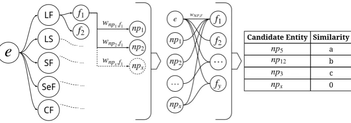
We assume that all noun phrases (NPs) are candidate entities and extract all of them from the unstruc-tured text3. Then, we record five features for each noun phrase (np) and model the data as a bipartite graph with NPs on one side and features on the opposite side. Ultimately, modeling the edges from multi-modal edge weights allow us to calculate the similarity between NPs and retrieve all sentences containing the most similar ones.

3.1 Noun Phrase Extraction (NPEx)

We POS tag and parse sentences to the form ([wi/posi ∀w∈W]). We then use the regular expressions

below to extract NPs, where JJs are adjectives, NNs are nouns (singular, plural, proper, etc.), and CDs are cardinal numbers (Santorini, 1990).

NP = JJs + NNs + CDs

JJs = (?:(?:[A-Z]\\w+ JJ )*) NNs = (?:[ˆ\\s]* (?:N[A-Z]*)\\s*)+ CDs = (?:\\w+ CD)?

3.2 Featurization

We automatically extract and record five kinds of features for each extracted noun phrase from text to create relationships between noun phrases. Following is the list of the diverse lexical, syntactic, and semantic features we derive:

1 Lexical Features (LF):

• Orthographic Form (OF): We abstract OF features from the actual word and obtain its type (i.e., numeric, alpha, alphanumeric, or other). Additionally, we classify the word as: all upper case, all lower case, title case, or mixed case.

• Word Shape (WS): We define WS to abstract the patterns of letters in a word as short/long word shape (SWS/LWS) features. In LWS, we map each letter to “L”, each digit to “D”, and retain the others unchanged. On the other hand, for SWS, we remove consecutive character

types. For example, LWS(“ABC-123”)→“LLL-DDD” and SWS(“ABC-123”)→“L-D”.

2 Lexico-Syntactic Features (LS):We use a skip-gram method to record the explicit LS-patterns surrounding each NP, i.e., for eachnpinswe record the patternwi−1+np+wi+1, wherew(.)

are the two words that precede and follownp.

3 Syntactic Features (SF):We use dependency patterns to abstract away from the word-order in-formation that we can capture using contextual and lexico-syntactic features. We use Stanford’s English UD neural network-based dependency parser (Chen and Manning, 2014) to extract uni-versal dependencies of NPs. For eachnpins, we record two dependency patterns of the NP that serve ingovernoranddependentroles.

4 Semantic Features (SeF):To capture the lexical semantics, we use WordNet (Miller, 1995) to get word senses and draw sense relations between NPs if they have the same sense class.

5 Contextual Features (CF):To capture the latent features, we use a Word2Vec embedding model (Mikolov et al., 2013) trained on the sentence poolSas the only bottom-up distributional seman-tics method. We exploit the word-context co-occurrence patterns learned by the model to induce the relational similarities between NPs.

The use of semantic (i.e., word senses) and contextual (i.e., word embeddings) features for sparse or domain-specific data (such as enterprise data) is not enough and sometimes not even possible due to unavailability (Tao et al., 2015). Therefore, we tried to use diverse features in a complementary manner

LF

LS

SF

SeF

...

Can d i d at e En t i t y Si m i l ar i t y

a

b

c

0

CF

...

...

...

Figure 1: The three stages of graph embedding for candidate entities ranking.

to capture as many meaningful relations between potential entities as possible. For example, the absence of SeF for domain specific entities, such as protein molecules or parts numbers, is compensated by the use of WS features (e.g., by drawing a relation between the NPs “IL-2” and “AP-1” which have the same SWS and LWS features).

3.3 Feature-Graph Embedding

We model edges in the bipartite graph by assigning a weightwbetween each pair of a noun phrasenand a featuref using one of the following weights:

w1n,f =Cn,f (4)

w2n,f =log(1 +Cn,f)[log|N| −log(|N|f)] (5)

w3n,f =log(1 +Cn,f)[log|N| −log(

X

ˆ n

Cn,fˆ )] (6)

whereCn,f is the co-occurrence count betweennandf,|N|is the number of NPs in our dataset,|N|f

is the co-occurrence count of all NPs withf, andP

ˆ

nCn,fˆ is the sum of all NP co-occurrences with the

featuref. Equations 5 and 6 are two variations of TFIDF where the latter is adapted to weigh the edges in (Shen et al., 2017; Rong et al., 2016).

3.4 Set Expansion

Data:e: input seed;S: text sentences

Result:N ={n}: ranked similar noun phrases

Start

ˆ

N =∅;// all noun phrases

F=∅;// all features

fors←Sdo

ˆ

N = ˆN ∪ExtractNounPhrases(s);

F =F ∪Featurize(Nˆ);// Sec. 3.2

end

G=BuildBipartiteGraph(Nˆ,F);

// Section 3.3

N =CalculateSimilarity(e,G);

// Equation 7 or 8

returnrank(N);

Algorithm 1:Entity Set Expansion Our method starts by taking a seed entityefrom

the annotator input, and returns a ranked list of similar NPs (see Algorithm 1). After construct-ing a graph usconstruct-ing the embeddconstruct-ing method men-tioned in the previous section (see Figure 1), we calculate the similarity between the seed entitye and all other noun phrasesN P sin the graphG using one of the following similarity methods:

Sim1(n1, n2|F) =

P

f∈F

wn1,fwn2,f

r P

f∈F

w2 n1,f

r P

f∈F

w2 n2,f

(7)

Sim2(n1, n2|F) =

P

f∈F

min(wn1,f, wn2,f)

P

f∈F

LF LS SF SeF

CF

Nou n Ph r ase Ran k

1 2

... ...

Nou n Ph r ase Ran k

... ...

3

... ...

9

... ...

... ...

Nou n Ph r ase Ran k

... ...

... ...

... ...

LF, LS, SF, SeF

LF, LS, SF, CF

LF, LS, SeF, CF

LF, SF, SeF, CF

...

Figure 2: Coarse features ensemble method for ranking candidate entities.

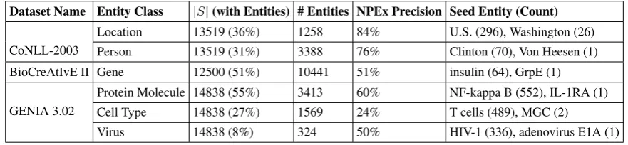
Dataset Name Entity Class |S|(with Entities) # Entities NPEx Precision Seed Entity (Count)

CoNLL-2003

Location 13519 (36%) 1258 84% U.S. (296), Washington (26)

Person 13519 (31%) 3388 76% Clinton (70), Von Heesen (1)

BioCreAtIvE II Gene 12500 (51%) 10441 51% insulin (64), GrpE (1)

GENIA 3.02

Protein Molecule 14838 (55%) 3413 60% NF-kappa B (552), IL-1RA (1)

Cell Type 14838 (27%) 1569 24% T cells (489), MGC (2)

Virus 14838 (8%) 324 50% HIV-1 (336), adenovirus E1A (1)

Table 1: Evaluation dataset statistics, noun phrase extraction accuracies, and seed entity counts.

whereSim(n1, n2|F)is the similarity between the two noun phrasesn1andn2given the set of features

F they have in common, and w(.,.) is the weight of the edge between the NPs and features (defined

using one of the Equations 4-6). Equation 7 is the cosine similarity and Equation 8 is the context-dependent similarity by (Shen et al., 2017). The difference between these two similarity measure is that higher cosine similarities implies that the two NPs are better aligned on many feature dimensions, while higher context-dependent similarities implies that the two NPs are significantly similar on some feature dimensions compared to others.

3.5 Feature Ensemble Ranking

Similar to the use in SetExpan (Shen et al., 2017), we ensemble the coarse features4 and rank NPs in sublists to reduce the effect of inferior features on the final ranking. The size of each sublist is equal to

|Fˆ| −1, whereFˆis the set of all features from Section 3.2.

M RR(n) =X

q∈Q

1

rank(n, q) (9)

We then use the mean reciprocal rank (MRR) from Equation 9 above, a form of rank aggregation, to find the final ranking of each noun phrasenusing its rank in each sublistq(see Figure 2).

4 Experiments and Results

4.1 Data Preparation

To test our framework while emulating the full experience of annotators, we use three publicly available gold standard datasets labeled for several entity classes (CoNLL-2003, GENIA 3.02, and BioCreAtIvE II). We tokenize documents into sentences, then query the emulator (which plays the role of annotators) to label sentences, thus avoiding the required annotation of full documents for better user experience. We require the emulator to label only a single entity class from each dataset, to avoid the complexity of multiple class annotations. Therefore, we created six versions of the datasets where only one class is kept in each version. Table 1 includes some statistics about the datasets. The percentage of sentences with entities of a given class shows the sparsity of those entities.

Location Person Gene Protein Cell Type Virus

Eq.4 Eq.5 Eq.6 Eq.4 Eq.5 Eq.6 Eq.4 Eq.5 Eq.6 Eq.4 Eq.5 Eq.6 Eq.4 Eq.5 Eq.6 Eq.4 Eq.5 Eq.6

Seed 1 Eq.7 0.37 0.40 0.50 0.23 0.23 0.30 0.00 0.03 0.13 0.17 0.23 0.20 0.27 0.50 0.53 0.20 0.13 0.17 Eq.8 0.63 0.73 0.73 0.03 0.17 0.20 0.03 0.07 0.07 0.43 0.43 0.53 0.17 0.23 0.23 0.07 0.10 0.07

Seed 2 Eq.7 0.33 0.33 0.57 0.53 0.40 0.30 0.63 0.63 0.63 0.17 0.60 0.27 0.10 0.20 0.13 0.07 0.03 0.03 Eq.8 0.57 0.70 0.63 0.47 0.37 0.37 0.60 0.57 0.60 0.07 0.30 0.30 0.07 0.07 0.07 0.03 0.10 0.03

Table 2: ESE performance (p@k). The use of TFIDF variant without co-occurrence summation (Equation 5), to weight the graph edges, and the context-dependent similarity (Equation 8), to measure the similarity between NPs, led to the bold-faced best performing combination.

Text

ESE

Input Seed

Auto Annotate

- Fast - Hyper Fast - Ultra Fast

Learn Model

t1 t2 t3 t4 t5 B-Cla I-Cla O B-Cla O

Sample Sentences Annotate

Human Intelligence

Task (HIT)

- Random-based - nSE-based

A B C

D E

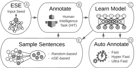
Figure 3: End-to-End system pipeline. Arrows represent paths can be followed to annotate text.

4.2 NPEx Evaluation

Since ESE method operates at an NP level, the performance of Noun Phrase Extraction (NPEx) signifi-cantly influences the overall performance of ESE. Table 1 includes the precision of NPEx method. In the future, ESE performance can be improved by enhancing the performance of candidate entities extraction through, for example, extracting noun phrases formed from typed-dependencies.

4.3 Entity Set Expansion (ESE) Evaluation

To test the influence of seed entity frequency on ESE performance, we manually picked two seeds, the most frequent and the least frequent among all noun phrases (See Table 1). Additionally, we varied the weighting measure of the graph edges to reflect different notions of feature relevance using one of Equations 4-6. Finally, we varied the similarity measure when ranking NPs (Equations 7 and 8).

We tested the performance of ESE with and without using the feature ensemble method in Section 3.5. We measured the precision of the method in ranking positive examples of entities similar to the seed entity (Seed 1 and Seed 2) in the topkNPs. We designed ESE to output thirty candidate entities (NPs) ranked based on the similarity to the seed term. Therefore, we calculated precision atk(p@k) where kis always 30. Table 2 shows the best results when using the feature ensemble method which is more stable than the non-ensemble one (due to lower standard deviation and non-zero precision). According to the results, the best combination in terms of the mean and standard deviation is obtained when using TFIDF (Eq.5) to weigh the edges and context-dependent similarity (Eq.8) to rank NPs. This shows that the uniqueness and the significant overlap of features between noun phrases were very important.

4.4 Full System Evaluation

We tested our pipeline on three different settings following three different paths in Figure 3:

1. All Random (AR):(E, B, C)∗, whereEis a random-based sampler.

2. ESE and AL (EAL):A, B, C,(E, B, C)∗, whereEis annSE-based sampler.

0% 10% 20% 30% 40% 50% 60% 70% 80%

Location Person Gene Cell-Type Virus Protein

Per

centage of P

ool Consumption

0.80 F-Score 0.90 F-Score 0.95 F-Score 1.00 F-Score

Figure 4: Percentage of sentences annotated while using EAL to reach different F-Scores.

Dataset Name Entity Class

EAL EAA Annotation Mode

@ 1.0 F FA HFA UFA

σ % cut F-Score (percentage cut)

CoNLL-2003

Location 0.97 55% 0.99 (46%) 0.93 (83%) 0.82 (91%)

Person 0.97 59% 0.99 (48%) 0.95 (81%) 0.85 (90%)

BioCreAtIvE II Gene 0.94 35% 1.00 (35%) 0.96 (50%) 0.89 (69%)

GENIA 3.02

Protein Molecule 0.99 33% 0.98 (36%) 0.87 (71%) 0.74 (85%)

Cell Type 0.99 62% 0.94 (70%) 0.82 (86%) 0.74 (91%)

Virus 0.94 24% 0.97 (79%) 0.89 (94%) 0.84 (96%)

Average 0.97 45% 0.98 (52%) 0.90 (78%) 0.81 (87%)

Table 3: Pipeline testing results of EAL and EAA annotation modes (see Section 2) showing the model confidence (σ), F-Scores, and percentage cut from the pool of sentences.

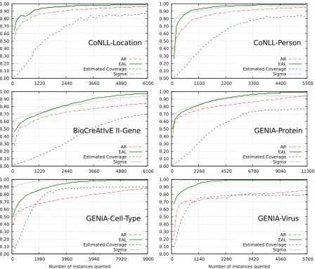
We iterate through the loop paths in the starred parentheses while sampling 100 sentences each time until we finish all sentences in the pool or reach full F-Score. In Figure 5, we show the performance of the first two settings (i.e., AR and EAL) in terms of F-Score. The use of AL and ESE methods outperformed random sampling all the time. ESE increased the performance of the base model by 35% F-Score on average, allowing us to reach 0.5 F-Score while the random sampler reached only 0.37 F-Score.

As shown in Figure 4, the percentage consumption of the sentence pool to reach up to 0.95 F-Score follows almost a linear growth. However, this cost grows exponentially if we want to reach 1.0 F-Score (needing on average around 33% more sentences). Practically speaking, we might want to trade the 5% F-Score improvement to significantly reduce manual labor.5

We used Jensen-Shannon divergence (Lin, 1991) to compare the curves corresponding to the perfor-mance of the estimated coverage method (Equation 3) and our online evaluation metricσ(Equation 2)

with the F-Score curve of EAL (see Figure 5). Our method σ outperformed the estimated coverage

method with a decrease of 96% in dissimilarity, which makes our method more reliable. Additionally, as shown in Table 3, on averageσgives an accurate estimation of the F-Score without labeled data, with an error margin of 3% on average, when reaching 1.0 F-Score (i.e., @ 1.0 F).6

Our EAL method also outperformed (Tsuruoka et al., 2008) on the three overlapping entity classes we tested on from the two datasets (Genia and CoNLL-2003). EAL needed 2800, 2900, and 400 fewer sentences to reach the same coverage as (Tsuruoka et al., 2008) for the Location, Person, and Cell-Type datasets, respectively.

Finally, for the last setting, we tested the system using the three auto-annotation modes (i.e., FA, HFA,

5_{This would, therefore, make the annotated data a silver standard instead of a gold standard.}

0.00 0.10 0.20 0.30 0.40 0.50 0.60 0.70 0.80 0.90 1.00

0 1220 2440 3660 4880 6100 CoNLL-Location AR EAL Estimated Coverage Sigma 0.00 0.10 0.20 0.30 0.40 0.50 0.60 0.70 0.80 0.90 1.00

0 1100 2200 3300 4400 5500

CoNLL-Person AR EAL Estimated Coverage Sigma 0.00 0.10 0.20 0.30 0.40 0.50 0.60 0.70 0.80 0.90 1.00

0 1220 2440 3660 4880 6100 BioCreAtIvE II-Gene AR EAL Estimated Coverage Sigma 0.00 0.10 0.20 0.30 0.40 0.50 0.60 0.70 0.80 0.90 1.00

0 2260 4520 6780 9040 11300

GENIA-Protein AR EAL Estimated Coverage Sigma 0.00 0.10 0.20 0.30 0.40 0.50 0.60 0.70 0.80 0.90 1.00

0 1980 3960 5940 7920 9900

F-S co re GENIA-Cell-Type AR EAL Estimated Coverage Sigma 0.00 0.10 0.20 0.30 0.40 0.50 0.60 0.70 0.80 0.90 1.00

0 1140 2280 3420 4560 5700 Number of instances queried

GENIA-Virus

AR EAL Estimated Coverage Sigma

Number of instances queried

Figure 5: Learning curves with different query strategies. Y-axis value for AR and EAL is the F-Score, and for Sigma and Estimated Coverage is the value from Equations 2 and 3, respectively.

and UFA) as shown in Table 3. While the auto-annotation mode can allow us to reduce up to 87% of the data pool, this drastic saving also reduces the accuracy of the learned model, achieving, on average, around 81% F-Score. Overall, our framework presents a trade off between coverage and annotation cost. The HFA auto-annotation mode shows the benefit, especially in a realistic enterprise setting, when we need to annotate 33% of the data to increase F-Score by only 10% (when comparing the on average performance of HFA with ESA) is unreasonable.

Table 3 appears to show FA being inferior to EAL in terms of the percentage cut for the Location class, for example. In reality FA reduced sentence annotation by 65% to reach 0.99 F-Score. But as our testing criteria demanded that we either reach 1.0 F-Score or finish all sentences from the pool, FA tried to finish the pool without any further performance improvement on the 0.99 F-Score.

5 Related Work

To extract sparse entities from texts and learn sequence models faster, our practical framework uses Active Learning (AL) for sequence labeling (Tomanek and Hahn, 2009; Settles and Craven, 2008), both as a method of sampling and to auto-annotate sentences. Our work encompasses entity extraction, Entity Set Expansion (ESE), corpora pre-annotation, auto-annotation, and AL.

Sadamitsu et al., 2012) where the system starts with a few positive examples of an entity class and tries to extract similar entities. Additionally, we use a richer set of features than those in (Gupta and Manning, 2014; Grishman and He, 2014; Min and Grishman, 2011) while training a CRF model and using it to find additional positive examples of a given entity class.

Methods such as (Sarmento et al., 2007) computes the degree of membership of an entity in a group of predefined entities called seed entities, where the class of each group is predefined. Their method does not focus on entity extraction, rather it focuses on detecting the class of entities during the evaluation step, which makes their method different from ours.

Regarding corpus annotation, many notable previous works such as (Lingren et al., 2013) use dictio-naries to pre-annotate texts. However, inaccurate pre-annotations may harm more than improve since they require an added overhead of modifications and deletions (Rehbein et al., 2009). Kholghi et al. (2017) and Tsuruoka et al. (2008) propose AL-based annotation systems. However, their work differs from ours in the following ways: (1)we propose a more accurate online evaluation method than theirs,

(2)we use ESE to bootstrap the learning framework collaboratively with a user-in-the-loop, and finally,

(3)we provide auto-annotation modes which reduces the number of sentences to be considered for an-notation and so allows for better usability of the framework.

6 Conclusions and Future Work

We presented a practical and effective solution to the problem of sparse entity extraction. Our frame-work builds supervised models and extracts entities with a reduced annotation cost using Entity Set Expansion (ESE), Active Learning (AL), and auto-annotation without compromising extraction quality. Additionally, we provided an online method for evaluating model confidence that enables flexible stop-ping criteria. In the future, we might consider evaluating different AL querying strategies and compare their performances and try a more sophisticated candidate entity extractors for entity set expansion.

References

Danqi Chen and Christopher Manning. 2014. A fast and accurate dependency parser using neural networks. In Proceedings of the 2014 conference on empirical methods in natural language processing (EMNLP), pages 740–750.

Laura Chiticariu, Yunyao Li, and Frederick R Reiss. 2013. Rule-based information extraction is dead! long live rule-based information extraction systems! InEMNLP, number October, pages 827–832.

Larry Smith et. al. 2008. Overview of biocreative ii gene mention recognition.Genome Biology, 9(2):S2, Sep.

Jenny Rose Finkel, Trond Grenager, and Christopher Manning. 2005. Incorporating non-local information into information extraction systems by gibbs sampling. InProceedings of the 43rd annual meeting on association for computational linguistics, pages 363–370. Association for Computational Linguistics.

Ralph Grishman and Yifan He. 2014. An information extraction customizer. In Petr Sojka, Aleˇs Hor´ak, Ivan Kopeˇcek, and Karel Pala, editors,Text, Speech and Dialogue, pages 3–10, Cham. Springer International Pub-lishing.

Sonal Gupta and Christopher D Manning. 2014. Improved pattern learning for bootstrapped entity extraction. In CoNLL, pages 98–108.

Mahnoosh Kholghi, Laurianne Sitbon, Guido Zuccon, and Anthony Nguyen. 2017. Active learning reduces annotation time for clinical concept extraction.International journal of medical informatics, 106:25–31.

Seokhwan Kim, Yu Song, Kyungduk Kim, Jeong-Won Cha, and Gary Geunbae Lee. 2006. Mmr-based active ma-chine learning for bio named entity recognition. InProceedings of the Human Language Technology Conference of the NAACL, Companion Volume: Short Papers, pages 69–72. Association for Computational Linguistics.

Todd Lingren, Louise Deleger, Katalin Molnar, Haijun Zhai, Jareen Meinzen-Derr, Megan Kaiser, Laura Stouten-borough, Qi Li, and Imre Solti. 2013. Evaluating the impact of pre-annotation on annotation speed and potential bias: natural language processing gold standard development for clinical named entity recognition in clinical trial announcements.Journal of the American Medical Informatics Association, 21(3):406–413.

Christopher D Manning, Mihai Surdeanu, John Bauer, Jenny Rose Finkel, Steven Bethard, and David McClosky. 2014. The stanford corenlp natural language processing toolkit. InACL (System Demonstrations), pages 55–60.

Tomas Mikolov, Ilya Sutskever, Kai Chen, Greg S Corrado, and Jeff Dean. 2013. Distributed representations of words and phrases and their compositionality. In Advances in neural information processing systems, pages 3111–3119.

George A Miller. 1995. Wordnet: a lexical database for english. Communications of the ACM, 38(11):39–41.

Bonan Min and Ralph Grishman. 2011. Fine-grained entity set refinement with user feedback. Information Extraction and Knowledge Acquisition, page 2.

Tomoko Ohta, Yuka Tateisi, Jin-Dong Kim, Sang-Zoo Lee, and Junichi Tsujii. 2001. Genia corpus: A semanti-cally annotated corpus in molecular biology domain. InProceedings of the ninth International Conference on Intelligent Systems for Molecular Biology (ISMB 2001) poster session, volume 68.

Ines Rehbein, Josef Ruppenhofer, and Caroline Sporleder. 2009. Assessing the benefits of partial automatic pre-labeling for frame-semantic annotation. InProceedings of the Third Linguistic Annotation Workshop, pages 19–26. Association for Computational Linguistics.

Xin Rong, Zhe Chen, Qiaozhu Mei, and Eytan Adar. 2016. Egoset: Exploiting word ego-networks and user-generated ontology for multifaceted set expansion. InProceedings of the Ninth ACM International Conference on Web Search and Data Mining, pages 645–654. ACM.

Kugatsu Sadamitsu, Kuniko Saito, Kenji Imamura, and Yoshihiro Matsuo. 2012. Entity set expansion using interactive topic information. InPACLIC, pages 108–116.

Beatrice Santorini. 1990. Part-of-speech tagging guidelines for the penn treebank project (3rd revision).Technical Reports (CIS), page 570.

Luis Sarmento, Valentin Jijkuon, Maarten de Rijke, and Eugenio Oliveira. 2007. More like these: growing entity classes from seeds. InProceedings of the sixteenth ACM conference on Conference on information and knowledge management, pages 959–962. ACM.

Burr Settles and Mark Craven. 2008. An analysis of active learning strategies for sequence labeling tasks. In Pro-ceedings of the conference on empirical methods in natural language processing, pages 1070–1079. Association for Computational Linguistics.

Jiaming Shen, Zeqiu Wu, Dongming Lei, Jingbo Shang, Xiang Ren, and Jiawei Han. 2017. Setexpan: Corpus-based set expansion via context feature selection and rank ensemble. InThe European Conference on Machine Learning and Principles and Practice of Knowledge Discovery in Databases (ECML-PKDD 2017).

Fangbo Tao, Bo Zhao, Ariel Fuxman, Yang Li, and Jiawei Han. 2015. Leveraging pattern semantics for extracting entities in enterprises. InProceedings of the 24th International Conference on World Wide Web, pages 1078– 1088. International World Wide Web Conferences Steering Committee.

Erik F Tjong Kim Sang and Fien De Meulder. 2003. Introduction to the conll-2003 shared task: Language-independent named entity recognition. InProceedings of the seventh conference on Natural language learning at HLT-NAACL 2003-Volume 4, pages 142–147. Association for Computational Linguistics.

Katrin Tomanek and Udo Hahn. 2009. Semi-supervised active learning for sequence labeling. InProceedings of the Joint Conference of the 47th Annual Meeting of the ACL and the 4th International Joint Conference on Natu-ral Language Processing of the AFNLP: Volume 2-Volume 2, pages 1039–1047. Association for Computational Linguistics.

Yoshimasa Tsuruoka, Jun’ichi Tsujii, and Sophia Ananiadou. 2008. Accelerating the annotation of sparse named entities by dynamic sentence selection. BMC bioinformatics, 9(11):S8.