ISSN: 1311-1728 (printed version); ISSN: 1314-8060 (on-line version) doi:http://dx.doi.org/10.12732/ijam.v32i1.9
CALCULATING THREE THERMAL COEFFICIENTS FROM ONE DATA SET
A. Kharab1§, F.M. Howari2, R.B. Guenther3 1 Dept. of Applied Mathematics
Abu Dhabi University, Abu Dhabi 59911, UAE 2 College of Natural and Health Sciences Zayed University, Abu Dhabi 59911, UAE
3 Dept. of Mathematics
Oregon State University, Corvallis 97331, OR, USA
Abstract: We study the problem of determining three thermal coefficients from one set data of a model problem rising in thermodynamics. This is an inverse problem, that is to coincide the solution of the differential equation with actual experimental results. The used method is based on minimizing the solution of the problem with the experimental data. Both the direct and inverse problems are described and numerical results are given.
AMS Subject Classification: 65P99
Key Words: inverse problem, parameters, heat, optimization
1. Introduction
The problem of finding the coefficients and parameters for thermodynamical problems when the solution is known is an inverse problem. To solve the inverse problem, one must first solve the direct problem, then solve the inverse problem for some coefficients and parameters. Solving such a problem therefore requires solving an optimization (minimization) problem, which is algorithmically more
Received: November 7, 2018 c 2019 Academic Publications
applications of the determination of parameters of sample material has seen tremendous growth in recent years. Inverse problems can be formulated in many mathematical areas and can be analyzed by many different computational techniques (see [15], [16], [17], [18], [19], [23], [24], [25], [26]).
In [1] the authors illustrate the full description of fractal-based techniques and their application to the solution of inverse problems for ordinary and partial differential equations. In [2] the authors give a description of an inverse elec-tromagnetic problem using a perturbation homotopy method combined with Gauss-Newton methods. In [3] the authors investigate a method for imposing two natural frequencies on a dynamic system consisting of an Euler-Bernoulli beam and carrying a single mass attachment. In [4] the authors use an algo-rithm to solve the problem of splicing the shredded paper. In [5] the authors describe an internal tidal model with experiments to investigate the estimation of spatially varying bottom friction coefficients.
The book by Evensen (2006) provides a good overview of many computa-tional aspects of the subject, reflecting the author’s experience in geophysical applications and related areas and provides a good entry point to some of the current research in this area. In [7] Kaipio and Somersalo introduce the Bayesian approach to inverse problems, especially in the context of differen-tial equations. There is a wide research literature in the area of parameter estimation (see [8]), as well as attempts to introduce the notions of parameter estimation.
Wave propagation problems in environmental applications such as seismic analysis, acoustic and electromagnetic scattering are described in [9] for both forward and inverse problems.
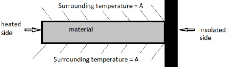
Figure 1: Geometry of the model problem.
2. The model problem
Our thermodynamic model problem consists on of a material that is insulated at x=L and with heat source located atx= 0.
We assume the sample is initially at the uniform temperature, A, heated by a lamp atx= 0 (see Fig. 1).
The sample is assumed to be homogeneous solid material. At the right end point is insulated, that is,
∂u
∂x(L, t) = 0.
At the left hand endpoint
W =−k∂u ∂x(0, t)
which means that the heat source is held constant during the course of the experiment.
Inside the sample, its temperature,u(x, t) is governed by the Newton type heat equation. So, the problem of findingu involves solving
ρc∂u
∂t(x, t) = k ∂2u
∂x2(x, t)−m(u−A), 0< x < L, t >0, (1) u(x,0) = A, 0≤x≤L,
∂u
∂x(L, t) = 0, t >0, ∂u
∂x(0, t) = −W/k, t >0,
We shall then determine parameters k, a,and α.If k, a,and α are known, thenc=k/(ρa) andm=ρcαare determined successively.
To simplify our problem, we make the change of variables to get the new problem for v(x, t)
ϕ(x) = W
2Lk(x−L) 2
u(x, t) = v(x, t) +ϕ(x), (3)
vt(x, t) = a vxx(x, t)−α v(x, t) (4) +[a ϕ′′(x)−α ϕ(x) +αA], 0 < x < L, t >0
vx(0, t) = 0, vx(L, t) = 0 (5) v(x,0) = A−ϕ(x). (6)
Once v(x, t) is known, thenu(x, t) is obtained from (3).
To solve the problem forv(x, t) we need to solve first the problem
zt(x, t) = a zxx(x, t)−α z(x, t), 0< x < L, t >0 (7) zx(0, t) = zx(L, t) = 0 (8)
z(x,0) = A−ϕ(x) (9)
which is done by settingz(x, t) =X(x)T(t).The explicit solution is then formed by several steps to obtain the eigenfunctions.
z(x, t) =e−αt
"
W L 6k −
∞ X n=1 2W kλ2 nL e−aλ2
ntcos(λ
nx)
#
(10)
and
ζ(x, t) = 4W αk
a+1 3L
2
1−e−αt
− ∞ X n=1 2W kLλ2
n(α+aλ2n)
h
1−e−(α+aλ2n)t
i
whereλn=nπ/L, n= 1,2, ....
Withz(x, t) and ζ(x, t) known,u(x, t) is obtained from the equation
u(x, t) =z(x, t) +ζ(x, t) +ϕ(x) +A. (12)
3. The inverse problem
There are three parameters that must be identified: a, k, and α. They all appear in the equations. the physically relevant parameters arek, c, mand the relationship are
k is the same,c=k/(ρa), m=ρcα,
whereρ is obtained independently.
Now the way the experiment is run as follows: Over a time period, 0 ≤
t ≤T,the lamp is turned on with a power Q watts. Then is turned off. The temperature then decreases until it reaches the ambient temperature along the full length of the sample. This actually means that the power of the lamp is a function of the timetso we should write
Q(t) =
W , 0≤t≤T,
0, t > T. (13)
Fort > T one has to reset the problem whereu(x, T) is the “initial” condi-tion and the boundary condicondi-tions are ux(0, t) = 0 andux(L, t) = 0.
We need data at several points. The way the identification go is that we have a solution to the initial problem for all time. The time dependent part, that is the so called transient part tends to zero rapidly so choose T so large that the transient part of the solution is negligible. The time independent part of the solution satisfies:
kuxx(x, t)−m[u(x, t)−A] = 0 ux(0, t) = −W/k ux(L, T) = 0.
The solution is
u(x) = √W
km
cosh(pm
kL) sinh(pm
kL) cosh(
r
m
kx)−sinh(
r
m
kx) +A. (14)
min
γ 0 [u( L
3, t)−U(t)]2dt (15)
is as small as possible. This will give the value for a.
4. Numerical results
In this section we will show some numerical results that determine the values of a, kandα and thereforeu(x, t) in the inverse problem. For the infinite series in equations (10) and (12) we took 100 terms to guarantee the convergence of the series. The integral in equation (15) is approximated using the trapezoidal rule. The least squares method along with Newton’s method for nonlinear equation are used for the minimization of equation (15).
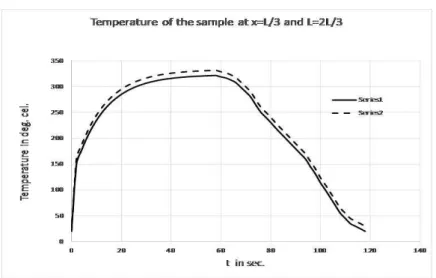
In this example we consider an unknown metal material with lengthL= 5 cm and density ρ = 2.71 g/cm3. The experiment was performed as described in Fig. 1 in the Laboratory of Zayed University, with the initial temperature of the sample A= 200c., W = 100 watts. The experiment was run for 60 sec. and then the lamp was turned off to let the sample cool down. The results of the experiment is shown in Fig. 2 giving the measured values of u(L/3, t) and u(2L/3, t),0≤t≤120.
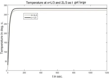
As t→ ∞, u(L/3) → 332.90c. and u(2L/3) → 322.60c (see Fig. 3) These values were used in Eqn. (14) to get the measured values for k= 203 W/cm-K andm= 1.45.These values are then used for the minimization of Eqn. (14) to obtain a= 81.36 cm/sec.and thereforec=k/(ρ∗a) = 0.92 W-s/Kg-K.
Nomenclature:
k= conductivity (W/cm-K) c= specific heat (W-s/Kg-K) ρ = density (g/cm3)
W = power (W/cm2)
Figure 2: Experimental results ofu(x, t) at x =L/3 (series 2) and x= 2L/3 (series 1.
5. Conclusion
This paper deals with the determination of three thermal coefficients from one set data of a model problem rising in thermodynamics. The present study shows that we can easily get the thermal coefficients of a material by solving an inverse problem that leads to an optimization problem. The model problem was presented and numerical results were given.
Acknowledgment.
The authors wish to acknowledge the support of Abu Dhabi University and Zayed University, Abu Dhabi, United Arab Emirates. The authors acknowledge the work done in this field by E. Wolff, founder of Precision Measurements and Instruments Corporation, Corvallis, Oregon, USA.
References
Figure 3: Temperature ast get large.
[2] L. Dingand, J. Cao, Electromagnetic nondestructive testing by pertur-bation homotopy method, Mathematical Problems in Engineering, 2014 (2014), Article ID 895159, 10 pages.
[3] F.M. Hosseini, N. Baddour, A structured approach to solve the inverse eigenvalue problem for a beam with added mass, Mathematical Problems in Engineering,2014 (2014), Article ID 292609, 12 pages.
[4] Peng Li and al., Reconstruction of shredded paper documents by feature matching,Mathematical Problems in Engineering,2014(2014), Article ID 514748, 9 pages.
[5] Y. Gao, A. Cao, H. Chen, X. Lv, Estimation of bottom friction coefficients based on an isopycnic-coordinate internal tidal model with adjoint method,
Mathematical Problems in Engineering, 2013 (2013), Article ID 532814, 11 pages.
[6] G. Evensen, Data Assimilation. The Ensemble Kalman Filter, Springer (2009).
[7] J. Kaipio, E. Somersalo, Statistical and Computational Inverse Problems, Springer (2005).
Phys-ical and BiologPhys-ical Processes, Chapman and Hall/CRC 1st Ed., Boca Ra-ton, FL (2009).
[9] I. Graham, U. Langer, J. Melenk, M. Sini (Eds.),Direct and Inverse Prob-lems in Wave Propagation and Applications, Ser.: Radon Series on Com-putational and Applied Mathematics, W. De Gruyter (2013).
[10] A. Kharab, E.G. Wolff, R.B. Guenther, Numerical investigation of an in-verse problem in thermodynamics, To appear in: Int. J. of Pure and Appl. Math., 120(2018).
[11] A. Kirsch,An Introduction to the Mathematical Theory of Inverse Problems of Applied Mathematical Sciences,120, Springer, NY, USA (2011). [12] F.D. Moura Neto, A.J. da Silva Neto,An Introduction to Inverse Problems
with Applications, Springer, New York (2013).
[13] A. Tarantola, Inverse Problem Theory and Methods for Model Parameter Estimation, SIAM, Philadelphia (2005).
[14] C.R. Vogel, Computational Methods for Inverse Problems, SIAM, New York (2002).
[15] H.W. Engl and W. Grever, Using the L-curve for determining optimal regularization parameters,Numerische Mathematik, 69, No 1 (1994), 25– 31.
[16] Y.L. Keung, J. Zou, An efficient linear solver for nonlinear parameter iden-tification problems, SIAM J. on Scientific Computing, 22, No 5 (2000), 1511–1526.
[17] J. Li and J. Zou, Amultilevel correction method for parameter identificatio,
Inverse Problems,23(2007), 1759–1786.
[18] J. Milstein, The Inverse Problem: Estimation of kinetic parameters, Chap-ter from: Modelling of Chemical Reaction Systems, Proc. of an Interna-tional Workshop, Heidelberg, Germany (Sept. 1980).
[19] A.N. Tychonoff, V.Y. Arsenin,Solution of Ill-Posed Problems, Winston & Sons, Washington, DC (1977).
lems,20, No 3 (2004), 977–991.
[23] H.E. Kunze, E.R. Vrscay, Solving inverse problems for ordinary differential equations using the Picard contraction mapping,Inverse Problems,15, No 3 (1999), 745–770.
[24] H. Kunze, D. la Torre, E.R. Vrscay, Solving inverse problems for DEs using the collage theorem and entropy maximization,Applied Mathematics Letters, 25, No 12 (2012), 2306–2311.
[25] H. Kunze, S. Gomes, Solving an inverse problem for Urison-type integral equations using Banach’s fixed point theore, Inverse Problems, 19, No 2 (2003), 411–418.