Algorithmic Stability and Meta-Learning

Algorithmic Stability and Meta-Learning

Andreas Maurer [email protected]

Adalbertstrasse 55

D-80799 M¨unchen, Germany

Editor: Tommi Jaakkola

Abstract

A mechnism of transfer learning is analysed, where samples drawn from different learning tasks of an environment are used to improve the learners performance on a new task. We give a gen-eral method to prove gengen-eralisation error bounds for such meta-algorithms. The method can be applied to the bias learning model of J. Baxter and to derive novel generalisation bounds for meta-algorithms searching spaces of uniformly stable meta-algorithms. We also present an application to regularized least squares regression.

Keywords: algorithmic stability, meta-learning, learning to learn

1. Introduction

We formally study the phenomenon of transfer, where novel tasks and concepts are learned more quickly and reliably through the application of past experience. Transfer is fundamental to human learning (see Robins, 1998, for an overview of the psychological literature) and offers a way to partially escape the implications of the No Free Lunch Theorem (NFLT).

The NFLT states that no algorithm is superior to another when averaged uniformly across all learning tasks. In a real environment, however, not all learning tasks occur equally likely. They are distributed according to some environmental distribution

E

, which is far from uniform. By gather-ing information on this distribution of tasks, a learner can possibly find an algorithm to outperform other algorithms, but, of course, only on average over the distribution

E

.

This mechanism of meta-learning has been analysed by Jonathan Baxter (1998, 2000) and there have been several successful experiments in practical machine-learning contexts (see Caruana, 1998; Thrun, 1996, 1998) and Section 6). In this paper we extend the results in Baxter (2000) and offer a general method to control the generalization error of meta-learning. We begin by reviewing some notions of learning theory.

Generalization error bounds. Statistical learning theory deals with data and hypotheses. A data point z may be an input-output pair z= (x,y)and a hypothesis c may be some function x_7→c(x), but for many theoretical results data and hypotheses can be arbitrary objects z and c, related only through a nonnegative loss function l(c,z)which measures how poorly the hypothesis c applies to the data point z. The familiar square loss l(c,(x,y)) = (c(x)₋y)2 is an example where z= (x,y) with y∈R_{and c : x7→c}(x)_∈R_.

task D. For a given hypothesis c the risk

R(c,D) =Ez∼D[l(c,z)] (1)

measures how poorly the hypothesis c is expected to perform on D.

A learning algorithm A takes a sample S= (z1, ...,zm)of data, drawn iid from the distribution D

defining the learning task, and computes a hypothesis A(S). The returned hypothesis should work well on the same learning task D, so we want the risk R(A(S),D)to be small. The quantity

ES∼Dm[R(A(S),D)] (2)

would be a natural measure for the performance of a given algorithm A with respect to a given learning task D.

Unfortunately the distribution D itself is generally unknown, so that we cannot compute or bound (2) directly. We do, however, know the sample S which was drawn from D, and we may give a performance guarantee for A conditioned on S, but for arbitrary D. Such a generalization error bound is typically given by specifying a two argument function B(δ,S), whereδ>0 is a confidence parameter, and the requirement that

∀D,Dm_{S : R(A(S),D)_≤B(δ,S)_{} ≥}1₋δ. (3) The bound above states that with high probability (1−δ) in S the learning-result A(S)will have risk bounded by B. Section 3 will give examples of generalization error bounds.

Meta-Learning. This paper describes a mechanism by which a sequence S= (S1, ...,Sn) of

samples, drawn from different learning tasks D1, ...,Dn, can be used to improve and predict the

performance of a learner on an unknown future task. We will give bounds analogous to (3) and also present a practical algorithm.

The crucial idea, due to J. Baxter (1998, 2000), is that the learning tasks Di originate from

an environment of tasks, which is a probability distribution

E

on the set of learning tasks. The encounter with a new learning task is thus modelled as a random event, a draw D∼

E

of a task D. Subsequent to the draw of D a sample S= (z1, ...,zm) may be generated by a sequence of m

independent draws from D. Let DE(S)be the overall probability for an m-sample S to arise in this

way,

DE(S) =ED∼E[Dm(S)].

The accumulation of experience is then modelled by n independent draws of samples Si∼DE,

resulting in the sample-sequence or meta-sample S= (S1, ...,Sn) (also called ’support sets’ by S.

Thrun, 1998, or(n,m)-samples by J. Baxter, 2000). The probability for S to arise in this manner is (DE)n(S)and depends completely on the environment

E

. We generally use m to denote the size of

the ordinary samples and n for the size of the meta samples. We also use bold letters D, S, l, etc to distinguish objects of meta-learning from the corresponding objects of ordinary learning D, S, l, etc.

A learners behaviour is formally described by a learning algorithm A. To say that the meta-sample S is used to determine the behaviour of the learner on future learning tasks can therefore be expressed in the equation

where A is a function which returns a learning algorithm for every meta-sample S. The object A will be called a meta-algorithm. Since A(S)is an algorithm we can train it with a sample S to obtain a hypothesis A(S) (S).

An example of a meta-algorithm is feature-learning where A selects a feature map to preprocess the input of a fixed algorithm. Another example is given in Section 6. In general, any method that adjusts the parameters of an algorithm on the basis of the experience made with other learning tasks can be regarded as a meta-algorithm.

To state generalization error bounds for meta-algorithms, we need to define a statistical mea-sure of the performance of an algorithm A with respect to an environment

E

, analogous to the risk R(c,D)of a hypothesis c with respect to a task D. The risk (1) measures the expected loss of a hypothesis for future data drawn from the task distribution D, so the analogous quantity for an algo-rithm should measure the expected loss of the hypothesis returned by the algoalgo-rithm for future tasks drawn from the environmental distribution

E

. A corresponding experiment involves the random draw of a task D from

E

, training the algorithm with a sample S drawn randomly and independently from D, and applying the resulting hypothesis to data randomly drawn from D. Formally

R(A,

E

) =ED∼E[ES∼Dm[R(A(S),D)]] =E_D∼E[E_S∼Dm[E_z∼D[l(A(S),z)]]]. (4)

The transfer risk R(A,

E

)measures how well the algorithm A is adapted to the environment

E

. If

E

is non-uniform the NFLT doesn’t apply, and we may hope to optimize R(A,

E

)in A.

If the environment was known, we could in principle select A so as to minimize (4), but the only available information is the past experience or meta-sample S. The situation is analogous to ordinary learning. Now suppose that A is a meta algorithm. The idea is to bound R(A(S),

E

)in terms of S with high probability in S, as S is drawn from the environment

E

for every environment

E

. Given S we can then reason that, regardless of

E

, the bound is true with high probability. Formally we seek a function B such that, given a confidence parameterδ,

∀

E

,(DE)n{S : R(A(S),

E

)≤B(δ,S)} ≥1−δ. (5)

The principal contribution of this paper is a general method to prove bounds of this type for different classes of meta-algorithms.

The Method. Given an algorithm A, let l(A,S)be an estimator for the risk of A(S)given the sample S= (z1, ...,zm). For example set l=lempwith the empirical estimator

lemp(A,S) = m

∑

i=1

l(A(S),zi).

We then write, using ES∼DE[f(S)] =ED∼E[ES∼Dm[f(S)]],

R(A(S),

E

)

=ES∼DE[l(A(S),S)] +ED∼E[ES∼Dm[R(A(S) (S),D)−l(A(S),S)]]

≤ES∼DE[l(A(S),S)] +sup

D,S0

To control the first term in the last line it suffices to prove a bound of the type

∀D_∈M1(Zm),Dn{S : ES∼D[l(A(S),S)]≤Π(δ,S)} ≥1−δ, (7) where D_∈M1(Zm)refers to any probability distribution on the set Zmof m-samples. Notice that (7) has exactly the same structure as an ordinary generalization error bound (3) where D has been repaced with D, S with S, A with A, l with l, and B withΠ. We therefore propose to use established results of learning theory to obtain the statement (7). Because it controls future values of the esti-mator, a two-argument functionΠsatisfying (7) will be called an estimator prediction bound for A with respect to the estimator l.

The simplest case, where a nontrivial estimator prediction bound can be found, occurs when A searches only a finite set of algorithms, but there are many other possibilities, some are listed in Section 3.

Suppose that we have established (7). To obtain (5) it will be sufficient to bound the second term in the last line of (6).

Methods for deriving ordinary generalization error bounds often use an intermediate bound on the estimation error

|R(A(S),D)₋l(A,S)_|,

valid for all distributions with high probability in S, for example by bounding the complexity of a hypothesis space searched by A. Such bounds lead to a general method to control the second term in (6) and to prove (5). Theorem 5 states a corresponding result, which is applied in Section 5.2 to improve on the results in (Baxter, 2000).

A second method to bound the estimation error in (6) involves the notion of algorithmic sta-bility. This method is less general but more elegant and often gives tighter bounds. Bousquet and Elisseeff (2002) have shown how generalization error bounds for learning algorithms can be ob-tained in an easy, elegant and direct way. Instead of measuring the size of the space which the algorithm searches, they concentrate directly on continuity properties of the algorithm in its depen-dence on the training sample. A learning algorithm is uniformlyβ-stable if the omission of a single example doesn’t change the loss of the returned hypothesis by more thanβ, for any data point and training sample possible. Many algorithms are stable and stable algorithms have simple bounds on their estimation error. Corresponding theorems can be found in (Bousquet, Elisseeff, 2002). The requirement of stability has been weakened and the results have been extended by Kutin and Nyogi (2002).

If for someβand all S the algorithm A(S)is uniformlyβ-stable, then the estimation term in (6) can be bounded in a particularly simple way, namely by 2β, as stated in Theorem 6.

Results. Algorithmic stability is also useful at a different level to prove that a meta-algorithm A has an estimator prediction bound. This can be done by appealing to Theorem 12 in (Bousquet, Elisseeff, 2002) (stated as Theorem 2 in Section 3). The following is an immediate consequence of this theorem in combination with our Theorem 6:

Theorem 1 Suppose the meta-algorithm A satisfies the following two conditions:

1. For every meta sample S= (S1, ...,Sn), let S\i be the same as S except that one of the Sihas

been deleted. Then for every S,S\iand every ordinary sample S we have

lemp(A(S),S)−lemp

A

S\i

,S

≤β

2. For every ordinary sample S= (z1, ...,zm), let S\i is the same as S except that one of the zi

has been deleted. Then for every meta sample S and every S and S\iwe have

l(A(S) (S),z)−l

A(S)S\i

,z

≤β.

Then for every environment

E

we have, with probability greater than 1₋δin the meta-sample S= (S1, ...,Sn)drawn from(DE)n, the inequality

R(A(S),

E

)_≤1

n

n

∑

i=1

lemp(A(S),Si) +2β0+ 4nβ0+M

r

ln(1/δ)

2n +2β. (8) The left hand side of the last inequality measures the expected performance of the algorithm A(S)for all, and potentially yet unknown, tasks of the environment

E

. The right side is composed of an empirical estimate and terms depending on the sample sizes n and m, the stability parameters

β0 _{andβand the confidence parameterδ. Ifβ}0≈_1/na_andβ≈_1/mb_{, with a>1/2 and b>0, the}

bound of the theorem becomes non-trivial.

We apply these results to a practical algorithm for least squares regression. This meta-algorithm is related to the Chorus of Prototypes introduced by Edelman (1995), so we call it CP-Regression. CP-Regression takes the meta-sample S= (S1, ...,Sn)and uses a primitive algorithm A0

to compute a set of corresponding regression functions h1, ...,hn. For any new input object x the

feature vector of x is then mixed with (or even replaced by) the vector(h1(x), ...,hn(x)). Finally

A(S)is defined to be regularized least squares regression with this modified input representation. We show that Theorem 1 applies to this meta-algorithm, withβ0≈_{1/n and}β≈_{1/m as required.}

CP-Regression can be implemented in practice and preliminary experiments seem to indicate that meta-learning gives a practical advantage over ordinary regularized least squares regression.

Outline of the Paper. In Section 2 we give a summary of the definitions and notation used in the paper. This section is intended as a reference for the reader. In Section 3 we show how to obtain estimator prediction bounds from standard results in learning theory. In Section 4 we derive transfer risk bounds for meta-algorithms. In Section 5 we attempt a comparison of our bounds to ordinary generalization error bounds and compare our method and results to the approach taken by J. Baxter (2000). In Section 6 we discuss regularized least squares regression, introduce CP-regression, analyse its properties and present some preliminary experimental results.

2. Definitions and Notation

This section is intended as a reference for the notation and definitions used in the paper.

Measurability. Any subset which we explicitely define on a measurable space will be assumed measurable, as will be any function. Thus for example ’F_⊆R_{’ is shorthand for the statement ’F⊆}R

and F is Lebesgue-measurable’. M1(X)will always denote the space of probability measures on a measurable space X . We supply M1(X)with anyσ-algebra containing theσ-algebra generated by the set of functions

for all bounded measurable functions f and all singleton sets{µ}for µ∈M1(X). In this way M1(X) becomes itself a measurable space and it makes sense to talk about M1(M1(X)).

Learning and Algorithms. Throughout Z will be a measurable space of data-points z_∈Z, C a space of hypotheses or concepts c_∈C and l : C_×Z_→[0,M]a loss function. Samples are polytuples S_∈S∞

m=1Zm, and learning algorithms are symmetric functions A :

∞ [

m=1

Zm_→C.

Symmetry, which will be essential for our use of stability, means that for any permutation π on

{1, ...,m_}and any S_∈Zmwe have A(π(S)) =A(S)whereπ(S)refers to the permuted sample

π(z1, ...,zm) = zπ(1), ...,zπ(m)

.

The set of such algorithms depends only on C and Z and will be denoted by

A

(C,Z). The hypothesis A(S)is what results when A is trained with S.

Learning Tasks and Risk. A learning task is specified by a probability measure D_∈M1(Z). Given such a task D and a hypothesis c_∈C and a loss function l we use

R(c,D) =Ez∼D[l(c,z)]

to denote the risk (=expected loss) of the hypothesis c in task D w.r.t. the loss function l. Generalization Error Bounds. A function B :(0,1]_×S∞

m=1Zm→[0,M]is a generalization error bound for the algorithm A_∈

A

(C,Z)with respect to the loss function l iff

∀D_∈M1(Z),∀δ>0,Dm{S : R(A(S),D)≤B(δ,S)} ≥1−δ.

Estimators and Algorithmic Stability. The leave-one-out estimator lloo and the empirical

estimator lempare the functions (the notation is from Bousquet, Elisseeff, 2002)

lloo,lemp:

A

(C,Z)×(Zm)→[0,M]

defined for A_∈

A

(C,Z)and S= (z1, ...,zm)∈Zmby

lloo(A,S) =

1 m

m

∑

i=1

lAS\i,zi

,

where S\i generally denotes the sample S with the i-th element deleted, and lemp(A,S) =

1 m

m

∑

i=1

l(A(S),zi).

Forβ>0 an algorithm A_∈

A

(C,Z)is called uniformlyβ-stable w.r.t. the loss function l if

|l(A(S),z)₋l

A

S\i

,z

for every m, for every S∈Zm,z∈Z and i∈ {1, ...,m}.

Environments and Induced Distributions. A meta-learning task is specified by an environ-ment

E

_∈M1(M1(Z))

which models the drawing of learning tasks D∼

E

. The environment

E

defines an induced distri-bution DE ∈M1(Zm), by

DE(F) =ED∼E[Dm(F)] for F⊆Zmmeasurable. (9)

The corresponding expectation for a measurable function f on Zmis then ES∼DE[f] =ED∼E[ES∼Dm[f(S)]].

The induced distribution DE models the probability DE(S)for an m-sample S to arise when a task

D is drawn from the environment

E

, followed by m independent draws of examples from the same distribution D. DE is not a product measure, but a mixture of symmetric product measures, and

therefore itself symmetric. Repeated, independent draws from DE give rise to meta-samples (see

below).

Transfer Risk. Given an environment

E

_∈M1(M1(Z)), an algorithm A∈

A

(C,Z)and a loss function l : C_×Z_→[0,M]the transfer risk of A in the environment

E

w.r.t. the loss function l is given by

R(A,

E

) =ED∼E[ES∼Dm[R(A(S),D)]].

It gives the expected risk of the hypothesis A(S)for a task D randomly drawn from the environment and the sample S randomly drawn from this task. It measures how poorly the algorithm A is suited to the environment

E

.

Meta-Samples and Meta-Algorithms. We use the letter S to denote a meta-sample, S= (S1, ...,Sn)∈(Zm)n. Such can be generated by a sequence of n independent draws from some

distri-bution D_∈M1(Zm), typically the distribution DE induced by an environment

E

, that is S∼(DE)n.

A

(

A

(C,Z),Zm) is the set of meta algorithms. That is for A _∈

A

(

A

(C,Z),Zm) and S_∈

S∞

n=1(Zm)n the object A(S) is the algorithm A=A(S)∈

A

(C,Z) which results from training A with the meta-sample S. Given an m-sample S, the object A(S) (S)is the hypothesis returned by the algorithm A(S), when trained with an ordinary sample S.

Estimator Prediction Bounds. A function Π:(0,1]_×S∞

n=1(Zm)n → [0,M] is an estima-tor prediction bound for the meta-algorithm A_∈

A

(

A

(C,Z),Zm) with respect to the estimator l :

A

(C,Z)_×(Zm)_→[0,M]iff

∀D_∈M1(Zm),∀δ>0,Dn{S : ES∼D[l(A(S),S)]≤Π(δ,S)} ≥1−δ. (10) An estimator prediction bound is formally equivalent to an ordinary generalization bound under the identifications Z_↔Zm, C_↔

A

(C,Z), l_↔l, A_↔A, B_↔Π.

Meta-Estimators. Given an estimator l :

A

(C,Z)_×(Zm_{)→[0,M]the empirical meta-estimator}

lempis the function

defined for A∈

A

(

A

(C,Z),Zm)and S= (S1, ...,Sn)∈(Zm)nby

lemp(A,S) =

1 n

n

∑

i=1

l(A(S),Si).

The meta-estimator lloois defined analogously. These definitions depend on the choice of the

esti-mator l itself. For example if l=lloothen

(lloo)emp(A,S) =

1 n

n

∑

i=1

lloo(A(S),Si).

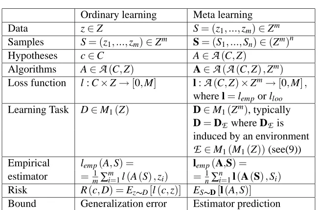
Ordinary learning Meta learning Data z_∈Z S= (z1, ...,zm)∈Zm

Samples S= (z1, ...,zm)∈Zm S= (S1, ...,Sn)∈(Zm)n

Hypotheses c_∈C A_∈

A

(C,Z)

Algorithms A_∈

A

(C,Z) A_∈

A

(

A

(C,Z),Zm) Loss function l : C×Z→[0,M] l :

A

(C,Z)_×Zm→[0,M],

where l=lempor lloo

Learning Task D_∈M1(Z) D∈M1(Zm), typically D=DE where DE is

induced by an environment

E

_∈M1(M1(Z))(see(9)) Empirical lemp(A,S) = lemp(A,S) =

estimator = 1

m∑ m

i=1l(A(S),zi) =_n1∑ni=1l(A(S),Si)

Risk R(c,D) =Ez∼D[l(c,z)] ES∼D[l(A,S)] Bound Generalization error Estimator prediction

Table 1: This table relates the descriptions of ordinary and meta-learning tasks.

An important object which is not mapped is the transfer risk R(A,

E

). Correspondingly an estimator prediction bound is not a generalization error bound for the transfer risk.

Covering Numbers. These definitions are taken from (Anthony, Bartlett, 1999). Let X be a set, X0⊆X . Forε>0 and a metric d on X the covering numbers

N

(ε,X0,d)are defined by

N

(ε,X0,d) =min

N_∈N_{:∃(x1, ...,xN)∈X}N_{,∀x∈X0,∃i,d(x,xi)≤}ε _.

For a class

F

of real functions on X and S= (x1, ...,xn)∈Xndefine

F

S⊆Rnby

F

_|S=_{(f(x1), ...,f(xn)): f ∈

F

},

and define, forε>0 and any given n,

N

1(ε,

F

,n) = sup

S∈Xn

where d1is the metric onRn_{defined by}

d1(x,y) = 1 n

n

∑

i=1

|xi−yi|.

Loss Function Classes. Let

H

_⊆C. The loss function class

F

(

H

,l) is the family of real functions

F

(

H

,l) =

z_∈Z_7→l(c,Z): c_∈

H

.

For

F

(

H

,l)we use the topology of pointwise convergence which it inherits as a subset of[0,M]Z. A set

H

_⊆C is called closed if

F

(

H

,l) is closed in this topology (and therefore also com-pact by Tychonoffs theorem). If

H

is closed then any finite linear combination of functions c_∈

H

_7→∑_iα_il(c,zi)attains minima and maxima in

H

.

For H_⊆

A

(C,Z)and a given estimator l :

A

(C,Z)_×Zm_→[0,M]we define an analogous (meta-) loss function class

F

(H,l) =_{S_∈Zm_7→l(A,S): A_∈H_}.

3. Estimator Prediction Bounds

In this section we give examples of estimator prediction bounds obtained from established results of statistical learning theory.

Selection from a Finite Set. Set the bound on the loss function M to be equal to 1 for simplicity and suppose that there is a finite set of hypotheses

H

=_{c1, ...,cK} ⊆C. Define the algorithm A for a sample S= (z1, ...,zm)∈Zmby

A(S) =arg min

c∈H

1 m

m

∑

j=1

l(c,zj).

A well known application of Hoeffdings inequality and a union bound (see e.g. Anthony, Bartlett, 1999) give, for anyδ>0,

∀D,Dm

(

S : sup

c_∈H

R(c,D)₋1

m

m

∑

j=1 l(c,zj)

≤ r

ln(K/δ) 2m

)

≥1₋δ, (11)

which gives the following generalization error bound for A:

∀D_∈M1(Z),∀δ>0,Dm{S : R(A(S),D)≤B(δ,S)} ≥1−δ with

B(δ,S) =lemp(A,S) + r

ln K+ln(1/δ) 2m .

Note that this bound also holds for every algorithm searching a finite set of hypotheses of cardinality at most K, that is for every algorithm with A(S)_∈

H

for all S and some set

H

with

H

≤K.

We now use the table at the end of the previous section. Substituting Zm_{for Z,}

_A

_{(C,Z)for C,}

l=lempor l=lloofor l and a finite set of algorithms{A1, ...,AK}for{c1, ...,cK},we arrive at the

Every meta algorithm A that such A(S)_{∈ {}A1, ...,AK}for all S= (S1, ...,Sn) has the estimator

prediction bound

∀D_∈M1(Zm),∀δ>0,Dn{S : ES∼D[l(A(S),S)]≤Π(δ,S)} ≥1−δ with

Π(δ,S) =lemp(A,S) + r

ln K+ln(1/δ)

2n . (12)

Selection from a Set of Bounded Complexity. Again with M=1 consider a subset

H

_⊆C. It follows from the analysis in chapter 17 in (Anthony, Bartlett, 1999) and Theorem 21.1 of the same reference, that the following holds for every 0<ε<1 and every distribution D on Z:

Dm

(

S_∈Zm:_∀c_∈

H

,

Ez∼D[l(c,z)]−

1 m

m

∑

j=1 l(c,zj)

≤ε )

≥1₋4N1

ε

8,

F

(

H

,l),2m

e−ε322m. ₍₁₃₎

which implies the following generalization error bound, valid for every algorithm A searching only the hypothesis space

H

:

B(δ,S) =lemp(A,S) +inf

t : 4

N

1

t

8,

F

(

H

,l),2m

e−32t2m ≤δ

. (14)

Suppose now that H_⊆

A

(C,Z)is a space of algorithms and fix an estimator l=llooor l=lemp.

Substituting Zmfor Z,

A

(C,Z)for C, l for l and H for

H

, and

F

(H,l)for

F

(

H

,l)in the above, we obtain analogous to (13):

For every 0<ε<1 and every distribution D on Zm:

Dm

(

S_∈(Zm)n:_∀A_∈H,

ES∼D[l(A,S)]− 1 n

n

∑

j=1

l(A,Sj) ≤ε )

≥1₋4N1

ε

8,

F

(H,l),2n

e−32ε2n.

Every meta-algorithm A such A(S)_∈H for all S has thus the estimator prediction bound

Π(δ,S) =lemp(A,S) +inf

t : 4

N

1

t

8,

F

(H,l),2n

e−t2n32 ≤δ

. (15)

Theorem 2 Let A∈

A

(C,Z)be uniformlyβ-stable. Then for any learning task D∈M1(Z)and any positive integer m, with probability greater 1₋δin a sample S drawn from Dm

l(A(S),D)_≤lloo(A,S) +β+ (4mβ+M) s

ln1_δ 2m and

l(A(S),D)_≤lemp(A,S) +2β+ (4mβ+M) s

ln1_δ 2m.

These bounds are good if we can show uniformβ-stability withβ≈_1/ma_{, with a>1/2. The}

notion of uniform stability easily transfers to meta-algorithms to give estimator prediction bounds. Fix an estimator l=lloo or l=lemp and suppose that the meta-algorithm satisfies the following

condition:

For every meta sample S= (S1, ...,Sn), if S0 is the same as S except that one of the Si has been

deleted, and for every ordinary sample S we have

l(A(S),S)−l A S0

,S≤β.

Theorem 2 then gives the estimator prediction bounds

Πloo(δ,S) =lloo(A,S) +β+ (4nβ+M) s

ln1_δ

2n (16)

and

Πemp(δ,S) =lemp(A,S) +2β+ (4nβ+M) s

ln1_δ

2n . (17)

4. Transfer Risk Bounds for Meta Algorithms

To derive the results in this section we need the following simple lemma, which can also be found in (Bousquet, Elisseeff, 2002).

Lemma 3 Let A_∈

A

(C,Z). Then for any learning task D_∈M1(Z) 1. We have ES∼Dm[l_loo(A,S)] =E_S0

∼Dm−1[R(A(S0),D)].

2. If A is uniformlyβ-stable then_|ES∼Dm[l_emp(A,S)]−E_S∼Dm[l_loo(A,S)]| ≤β.

Proof Using the permutation symmetry of A and of the measure Dmwe get

ES∼Dm[l_loo(A,S)] = 1

m

m

∑

i=1 ES∼Dm

h

l

A

S\i

,zi i

= 1

m

m

∑

i=1

ES0_∼Dm−1

Ez∼D

l A S0,z

= E_S0_∼Dm−1

Also

|ES∼Dm[l_emp(A,S)−l_loo(A,S)]|

≤_m1 m

∑

i=1

ES

h

l(A(S),zi)−l

AS\i,zi i

≤_m1 m

∑

i=1

|ES[β]|=β.

Suppose now that we have an estimator prediction bound Π for the meta-algorithm A with respect to the estimator l, so that, for allδ>0,

∀D_∈M1(Zm),Dn{S : ES∼D[l(A(S),S)]≤Π(δ,S)} ≥1−δ, (18) where the estimator l :A(C,Z)_×Zm_→[0,M]refers to either lempor lloo. We have outlined several

ways to obtain such bounds in Section 3.

When l=lloothe bound (18) is already powerful by itself. By the definition of DE and the first

conclusion of Lemma 3 we have

ES∼DE[lloo(A(S),S)] = ED∼E[ES∼Dm[lloo(A(S),S)]]

= ED∼EES0_∼Dm−1

R A(S) S0

,D

.

Substituting DE for D in (18) we conclude

Theorem 4 If the meta-algorithm A satisfies the estimator prediction bound (18) with l=lloothen

for every environment

E

, with probability greater than 1₋δin the meta sample drawn from(DE)n

we have

ED∼E[ES∼Dm−1[R(A(S) (S),D)]]≤Π(δ,S). (19)

The left side of (19) is not quite equal to the transfer risk R(A,

E

). Here is a first application of this bound: Let_{A1, ...,AK}be a finite collection of algorithms. For any meta sample S= (S1, ...,Sn)

define A(S)to be

A(S) =arg min

A∈{A1,...,AK}

1 n

n

∑

i=1

lloo(A,Si).

The meta-algorithm A selects the algorithm with the lowest leave-one-out error on average over the meta-sample. Applying the estimator prediction bound (12) for this type of algorithm in combina-tion with (19) above then gives, for any

E

and with probability greater than 1₋δin the meta sample drawn from(DE)n,

ED∼E[ES∼Dm−1[R(A(S) (S),D)]]≤

1 n

n

∑

i=1

lloo(A(S),Si) + r

ln(K/δ)

2n . (20) A similar result should hold if lloois replaced by any other, nearly unbiased estimator. A popular

generalization performance of an algorithm. If we chose from a finite set of candidates the algorithm A(S)which performs best on average over the test data in S, when trained with the training data in S, then we are implementing a version of the above meta-algorithm, and a corresponding version of (20) gives a probable performance guarantee for A(S)on future learning tasks drawn from the same environment as S.

For more sophisticated meta-algorithms we need to consider the case l=lemp. In this case

an estimator prediction bound only bounds the expected empirical error lemp(A(S),S) of A(S)

for a sample S drawn from DE, but it does not give any generalization guarantee for the hypothesis

A(S) (S). For example A(S)could be some single-nearest-neighbour algorithm for which we would have lemp(A(S),S) =0 for almost all S, but A(S)would have poor generalization performance.

Recall the decomposition of the transfer risk (6) in the introduction: R(A(S),

E

)

≤ES∼DE[l(A(S),S)] +sup

D,S0

E_S∼DmR A S0,D−l A S0,S.

The estimator prediction bound controls the first term above, so it remains to bound the second term which is independent of S. We need to bound the expected estimation error of the estimator l uniformly for all distributions D and all algorithms A(S)for all meta-samples S.

Theorem 5 Suppose the meta-algorithm A has an estimator prediction boundΠwith respect to the estimator l=lemp, and that for everyη>0 there is a number B(η)such that for every distribution

D_∈M1(Z), and every meta-sample S we have

Dm_{S :_|R(A(S) (S),D)₋lemp(A(S),S)| ≤B(η)} ≥1−η. (21)

Letε=inf_η(B(η) +Mη). Then for every environment

E

, with probability greater than 1₋δin S as drawn from(DE)nwe have

R(A(S),

E

)_≤Π(δ,S) +ε.

Proof For any D, S and arbitraryηwe have ES∼Dm[R(A(S) (S),D)]

≤ES∼Dm[l_emp(A(S),S)] +E_S∼Dm[|R(A(S) (S),D)−l_emp(A(S),S)|] ≤ES∼Dm[l_emp(A(S),S)] +B(η) +Mη,

where (21) was used in the last inequality. Taking the expectation D∼

E

gives R(A(S),

E

) = ED∼E[ES∼Dm[R(A(S) (S),D)]]

≤ ED∼E[ES∼Dm[l_emp(A(S),S)]] +ε

= ES∼DE[lemp(A(S),S)] +ε

≤ Π(δ,S) +ε,

The condition (21) is often satisfied, typically with B(δ)decreasing as ln(1/δ)inδand as m−1/2 in m, so we should get a boundεdecreasing about as quickly aspln(m)/m. Using the results in Section 3, now on the level of ordinary learning, we see that the above theorem can be applied

• if every A(S)selects a hypothesis from a finite set

H

(S)of choices with

H

(S)

≤K for all

S. This follows from (11) The

H

(S)may of course be different for different S..

• if every A(S)selects a hypothesis from a set

H

(S)_⊆C with uniformly bounded complexities. Here we use (13). An application is given in Section 5.2.

• if every A(S)is uniformlyβ-stable withβ≈_{1/m. This follows from Theorem 2.}

In the last case we can give a much better bound, where the additional error termεis often of order 1/m:

Theorem 6 Suppose the meta-algorithm A has an estimator prediction bound Πwith respect to the estimator l=lemp, and that for someβthe algorithms A(S)are uniformlyβ-stable for every

meta-sample S. Then for any environment

E

andδ>0, with probability greater than 1−δin S as drawn from(DE)n

R(A(S),

E

)_≤Π(δ,S) +2β. Proof We have

ES∼Dm[R(A(S) (S),D)] ≤ E_S0_∼Dm−1

R A(S) S0,D+β = ES∼Dm[l_loo(A(S),S)] +β ≤ ES∼Dm[l_emp(A(S),S)] +2β,

where the first inequality follows directly from uniform stability and the next lines follow from Lemma 3. Taking the expectation D∼

E

and using the estimator prediction bound (18) with DE in

place of D gives the result in just as in the proof of the previous theorem.

Theorem 1 now follows immediately from Theorem 6 and from the estimator prediction bound (17) in Section 3. In Section 6 an application of this theorem to a practical meta-learning algorithm is discussed.

The estimator prediction boundΠ(δ,S)will typically depend on the size n of the meta-sample S= (S1, ...,Sn), and not on the size m of the constituting samples Si. One may therefore wonder, how

we can have an m-dependence of the estimation error as 2β(often order 1/m), while in Theorem 2 (Bousquet, Elisseeff, 2002) it is 2β+O

p

1/m

. The reason for this difference is that to bound the transfer-risk in the above proof we only need to bound the expectation in S of the random variable R(A(S) (S),D), whereas the proof of Theorem 2 in (Bousquet, Elisseeff, 2002) needs to use McDiarmid’s concentration inequality to bound this random variable itself with high probability in S, which is where the O

_p

1/m

5. Comparison to Other Results

In this section we relate our results to others, beginning with a comparison to ordinary generaliza-tion bounds. Then we compare our method to the approach taken by J. Baxter (2000) where the generalization of meta-algorithms is also studied.

5.1 Comparison to Ordinary Generalization Error Bounds

Are our results better or worse than ordinary generalization error bounds? This question is at the same time very important and very imprecise, because the two kinds of results refer to different objects and situations.

The ordinary generalization error bound (examples in Section 3) applies to a situation where a sample S has already been drawn from an unknown task D and the estimator lemp(A,S)already has

a definite value. It typically has the structure

∀D,Dm_{S : R(A(S),D)_≤lemp(A,S) +ε0} ≥1−δ whereε0is a bound on the estimation error. Oftenε0≈

p

1/m.

Our bounds on the other hand apply to a situation where only the meta-sample S is known, and typically have the structure

∀

E

,(DE)nS : R(A(S),

E

)≤Π(δ,S) +ε0₀ ≥1−δ

whereΠ(δ,S)is the estimator prediction bound and ε0₀ is again a bound on the estimation error, uniformly valid for all algorithms A=A(S)for any S.

To getε0₀our method always requires some condition (uniform bounds on estimation errors,β -stability) on the algorithms A(S), which is also sufficient to prove an ordinary generalization error bound for such algorithms A(S). The corresponding estimation errors are about the same in our bounds and in the ordinary generalization error bounds. In case of Theorem 5 our ε0₀ is slightly worse than that of the ordinary bound (i.e.pln(m)/m vsp1/m), in case of Theorem 6 it is actually better (2βvs 2β+O

_p

1/m

). Let’s ignore these differences and putε0=ε00. Comparing the two bounds therefore involves a comparison of the estimator prediction bound Π(δ,S) to a ’generic’ value of the estimator lemp(A,S).

Our boundΠ(δ,S)has the disadvantage that it contains an additional error of meta-estimation. But as the size n of the meta-sample S becomes large, corresponding to an experienced meta-learner, this additional term tends to zero, andΠ(δ,S)is likely to win over the ’generic’ lemp(A,S), because

A(S)is likely to outperform the ’generic’ algorithm A on the meta-sample S. To make this precise we have to give more meaning to the word ’generic’.

While it is easy to define a generic value of S (simply taking S∼_{DE if some environment}

E

is given), it is not so clear how we should pick a generic algorithm A. For simplicity consider a finite set of algorithms_{A1, ...,AK}. We should select A uniformly at random from this set to obtain a

generic algorithm. The generic value of lemp(A,S)is then

Γ=ES∼DE

"

1 K

K

∑

k=1

lemp(Ak,S) #

The meta algorithm to consider for comparison is A(S) =arg min

A∈{A1,...,AK}

1

n_S

∑

_∈Slemp(A,S)

with the estimator prediction bound

ES∼DQ[lemp(A(S),S)] ≤ K

min

k=1 1

n_Si

∑

_∈Slemp(Ak,Si) +

r

ln(K/δM)

2n

= Π(δM,S), (22)

whereδMis the confidence parameter associated with the draw of the meta-sample S. Now let

∆(S) = 1

K

K

∑

k=1 1

n_S

∑

_∈Slemp(Ak,S)−

K

min

k=1 1

n_S

∑

_∈Slemp(Ak,S).

∆(S) will be positive unless all algorithms behave the same on the meta-sample, in which case it is zero and meta-learning is indeed pointless (essentially an empirical instantiation of the NFLT). With the bound M on the loss function equal to 1, an application of Hoeffding’s inequality gives, with probability greater than 1₋δM in a meta sample S drawn from(DE)n,

1 n_S

∑

_∈S

1 K

K

∑

k=1

lemp(Ak,S)≤Γ+ r

ln(1/δM)

2n , so with probability greater than 1₋2δM in the meta-sample S we have

Γ−Π(δM,S)≥∆(S)− p

ln(1/δM) + p

ln K+ln(1/δM) √

2n , (23)

in addition to validitiy of our bound (22). So for large meta-samples S our bounds will very probably be true and better than the generic value of ordinary generalization bounds by a margin of roughly

∆(S).

For a practical perspective consider image recognition, when the tasks in the support of

E

share a certain invariance property (say image rotation), and there is only one algorithm in_{A1, ...,AK} having this invariance property. We can then expect the wrong algorithms to have fairly large losses for a given meta sample S, so that∆(S)will have order≈_1.

5.2 Comparison to the Bias Learning Model

The approach taken in Baxter (2000) can be partially reformulated in our framework. We will consider only ERM-algorithms in

A

(C,Z)which have the form

AH(S) =arg min

c∈H

1

analysis in (Baxter, 2000) does not exploit the advantages of regularisation and we stick to ERM for definiteness and motivation.

The traditional method to give generalization error bounds for such algorithms is described in (Anthony, Bartlett, 1999) or (Vapnik, 1995) and involves the study of the complexity of the function space

F

_H =

z_7→l(c,z): c_∈

H

in terms of covering numbers or related quantities, and proceeds to prove a uniform bound on the estimation error, such as (13) in Section 3, valid for all c_∈

H

, and with high probability in the sample S. This leads to corresponding generalization error bounds. We have sketched a version of this approach which can be applied both to ordinary and to meta algorithms in Section 3.

The choice of the hypothesis space

H

completely defines the algorithm (24). A collection of such algorithms can therefore be viewed as a familyH_{of closed subsets}

H

_⊆C which define the algorithms AH by virtue of formula (24). A corresponding meta-algorithm takes a meta-sample

S, sampled from an environment

E

as usual, and returns an algorithm A(S) =AH(S) for some hypothesis space

H

(S)_∈H_{. The meta-algorithm can thus be equivalently considered as a map}

S_→

H

(S)or

H

:

∞ [

n=1

(Zm)n_→H_.

Such a meta-algorithm effectively learns the hypothesis space

H

(S), and in (Baxter, 2000) it is called a bias learner. For the remainder of this section takeH_{to be fixed and let A be any}

meta-algorithm defined by the ERM formula A(S) =AH(S) for some map S7→

H

(S)∈H. We also assume the bound M on the loss function to be equal to 1.

In our framework it is natural to study covering numbers for the space of algorithms H_H=

AH :

H

∈H

and use them to derive an estimator prediction bound (15) as outlined in Section 3. Imposing a uniform bound on the complexities of the hypothesis spaces in H _{then allows the application}

of Theorem 5. Putting together the estimator prediction bound (15), the uniform bound on the estimation error (13) and Theorem 5, we arrive at

Corollary 7 Let

ε0=inf

γ>0

(

γ+4 sup

H_∈H

N

₁γ

8,

F

(

H

,l),2m

e−γ2m/32

)

and, forδ>0,

ε1=inf

t : 4

N

₁t

8,

F

(H,l),2n

e−32t2n ≤δ

.

Then for any environment

E

, with probability at least 1₋δin the draw of a meta-sample S from

(DE)n, we have

R

AH(S),

E

≤1

n_Si

∑

_∈Slemp

AH(S),Si

+ε1+ε0.

Corollary 8 For any 0<ε<1,δ>0, if

n_≥128

ε2 ln

4

N

_{1 16}ε,

F

(HH,lemp),2n

δ

!

(25)

and

m_≥512

ε2 ln

4 sup_H∈H

N

_{1 32}ε ,

F

(

H

,l),2m

ε

!

, (26)

then for any environment

E

, with probability greater thanδin the draw of a meta-sample S from

(DE)n, we have

RAH(S),

E

≤1

n_Si

∑

_∈Slemp

AH(S),Si

+ε.

J. Baxter (2000) also defines capacities forH_{, but aims at giving a bound on}

sup

H_∈H

ED∼E

inf

c∈HR(c,D)

−1

n_Si

∑

_∈Slemp(AH,Si)

valid with high probability in S as drawn from(DE)nfor any

E

. A corresponding bound on

erE(

H

(S)):=ED∼E

inf

c∈H(S)R(c,D)

(27)

(which in Baxter, 2000, is called the generalization error of the bias learner), results. This is Theorem 2 in (Baxter, 2000). The expression (27) is the expected risk of the optimal hypothesis in

H

(S)as D is drawn from the environment.

The inequality

erE(

H

(S)) = ED∼E

ES∼Dm

inf

c∈H(S)R(c,D)

≤ ED∼E

h

ES∼Dm h

RAH(S)(S),D

ii

= R

AH(S),

E

(28) shows that our bounds on the transfer risk also provide bounds on (27). Note however that a bound on (27) does not itself guarantee generalization, because we may not find the optimal hypothesis from a finite future sample. This is similar to the estimator prediction bounds in our approach and contrary to our bounds on the transfer risk.

In Theorem 3 of Baxter (2000) the capacity of a given

H

is used to formulate a uniform bound on the estimation error of the hypotheses in

H

similar to (13). If corresponding capacity bounds held for all hypothesis spaces

H

_∈H_{, a bound on the transfer risk RAH}

(S),

E

bounds on the sample complexities look similar. This is not surprising since both derivations of bounds are rooted in the same classical method (see e.g. Vapnik, 1995).

The sample complexity bounds on the m-sample depending on the uniform capacity bound are then essentially the same in Baxter (2000) as in (26) (if we disregard that Baxter, 2000, imposes additional conditions on m in Theorem 2). For a comparison we therefore focus on the sample complexity bounds on the size n of the meta-sample. In Baxter (2000) Theorem 2, to get

erE(

H

(S))≤

1

n_Si

∑

_∈Slemp

AH(S),Si

+ε

with probability at least 1₋δin S, it is required that n_≥256

ε2 ln

8C ₃₂ε,H∗

δ , (29)

and there is an additional condition on m.

To compare (29) with our bound (25), we disregard the constants (which are better in (25)) and concentrate on a comparison of the complexity measures C(ε,H∗_)and

N

1(ε,

F

(HH,lemp),n).

In (Baxter, 2000) the capacity C(ε,H∗_{)is defined as follows: For}

H

_∈H_{define a real function}

H

∗_{on M1(Z)by}

H

∗(D) = inf

c∈HR(c,D).

In (Baxter, 2000) there are assumptions to guarantee that

H

∗_{is measurable on M1(Z), and since it} is obviously bounded we have

H

∗_∈L1(M1(Z),Q)for any probability measure Q∈M1(M1(Z)). Use dQto denote the metric in L1(M1(Z),Q)and denote

H∗₌

H

∗:

H

_∈H _.

Then

C(ε,H∗_{) = sup}

Q∈M1(M1(Z))

N

(ε,H∗_,dQ).

It turns out that our complexity measures are bounded by those in Baxter (2000). Proposition 9 For allε, n

N

₁(ε,

F

(HH,lemp),n)≤C(ε,H∗).

Proof For a sample S= (z1, ...,zm)∈Zm use DS to denote the empirical distribution DS∈M1(Z) induced by S:

DS=

1 m

m

∑

i=1

δzi,

whereδzis the unit mass concentrated at z∈Z. Note that for

H

∈Hwe have

H

∗(DS) = inf c∈H

1 m

m

∑

i=1

l(c,zi) =lemp(AH,S).

For a meta-sample S= (S1, ...,Sn)∈(Zm)nuse QSto denote the empirical distribution QS∈M1(M1(Z)) induced by S:

QS= 1 n

n

∑

i=1

whereδDis the unit mass concentrated at D∈M1(Z).

Now take any meta-sample S= (S1, ...,Sn)∈(Zm)nand let N=

N

(ε,H∗,dQS). Then there is a set of functions_{Ψ1, ...,ΨN} ⊆L1(M1(Z))such that for every

H

∈Hthere is some i such that

ε ≥ dQS(

H

∗,Ψi)

= 1

n

n

∑

j=1

H

∗ D_Sj

−Ψi DSj

= 1

n

n

∑

j=1

l_emp(A_H,S_j)−Ψ_i D_Sj

. (30)

On the other hand we have

F

(H_H,lemp)|S=

(lemp(AH,S1), ...,lemp(AH,Sn)):

H

∈H ,

so, setting xi∈Rnwith(xi)j=Ψi DSj

, we see from (30) that every member of

F

(H_H,lemp)|Sis within d1-distanceεof some xi. It follows that

N

(ε,

F

(HH,lemp)|S,d1)≤

N

(ε,H∗,dQS), whence

N

₁(ε,

F

(H_H,lemp),n) = sup

S∈(Zm₎n

N

(ε,

F

(H_H,lemp)|S,d1)

≤ sup

S_∈(Zm₎n

N

(ε,H∗_,dQ

S)

≤ sup

Q_∈M1(M1(Z))

N

(ε,H∗_,dQ)

=

C

(ε,H∗₎

We can conclude that our bounds are normally applicable when those in (Baxter, 2000) are. It may however happen, that our covering numbers increase polynomially in n, in which case we still get tight bounds, but the capacities in (Baxter, 2000) are infinite.

6. A Meta-Algorithm for Regression

In this section we present a meta-learning algorithm for function estimation. The algorithm is based on regularized least-squares regression, or ridge regression (as in Bousquet, Elisseeff, 2002, or Christianini, Shawe-Taylor, 2000) and preliminary experiments appear promising.

To implicitly also define a ’kernelized’ version of the algorithm, we describe it in a setting where the input space is a subset

X

of the unit ball_{kx_{k ≤}1_}in a separable, possibly infinite dimensional Hilbert space H, with an appropriately defined inner product.

As a hypothesis or concept space we consider the bounded linear functionals h on H which can be identified with members h_∈H via the action of the inner product h(x) =_hh,x_iin H.

As a loss function we use l : H_×Z_→R_{+given by}

l(h,(x,y)) = (_hh,x_{i −}y)2.

This loss function is unbounded contrary to what is generally required in this paper. It will however turn out that the effective hypothesis space searched by the algorithms in this section is the ball

kh_{k ≤}λ−1/2 whereλis the regularization parameter introduced below. 6.1 Regularized least squares Regression

A standard algorithm A_∈A(H,Z)for this type of problem is defined as follows: Let S= (z1, ...,zm) =

((x1,y1), ...,(xm,ym))∈Zmbe a sample. We write, for h∈H,

L(h) = 1

m

m

∑

i=1

(_hh,x_{ii −}yi)2+λkhk2

and define

A(S) =arg min

h∈HL(h). (31)

Note thatλ_kA(S)_k2_≤L(A(S))_≤L(0)_≤1 so_kA(S)_{k ≤}λ−1/2_{. The effective hypothesis space is} then_kh_{k ≤}λ−1/2 , as claimed above. Thus_|hh,x_{i| ≤}λ−1/2 and the loss function is bounded by

λ−1_.

Any component of h perpendicular to all the xi will only increase L, so we may assume that

A(S)is in the subspace generated by_{x1, ...,xm}, in other words

A(S) =

m

∑

i=1

αixi (32)

for some (possibly non-unique) vectorα_∈Rm_{. To find}α_{we substitute (32) in L and equate the}

gradient to zero. The result of this well known computation is the formula

(G+mλI)α=y (33) where Gi j =

xi,xj

is the Gramian matrix, here considered as an operator onRm_{, I =}δ

i j is the

identity, and y= (y1, ...,ym) the set of target values in the sample, here considered as a vector

y_∈Rm_{. Equation (33) can be efficiently solved for}α _{using the Cholesky decomposition method.}

The formula for the empirical loss of A(S)is, using (32) and (33) lemp(A,S) =

1 m

m

∑

i=1

((Gα)_i−yi)2

= 1

m

m

∑

i=1

(((G+mλI)α)_i−yi−mλαi)2

= 1

m

m

∑

i=1

(₋mλαi)2

= mλ2

m

∑

i=1

α2

i. (34)

It follows from example 3 in (Bousquet, Elisseeff, 2002) that the algorithm A so defined is

6.2 A Meta-Algorithm

Consider now a meta sample S= (S1, ...,Sn), drawn from(DE)nfor some environment

E

, and

sup-pose that we have used some ’primer’ algorithm A0 (for example the regression algorithm above for an appropriate value of λ=λ0) to train corresponding regression functions hk =A0(Sk)∈H.

The sequence of vectors (A0(S1), ...,A0(Sn)) = (h1, ...,hn) in some way contains our experiences

with the environment

E

. The idea of the meta-algorithm is now to use the hk as additional

fea-tures to describe a given new data-point x. We do this by combining the n-dimensional vector

(h1(x), ...,hn(x))with the existing description x∈H.

The intuitive motivation is that we expect the hi to already describe relevant properties

(sym-metries, elimination of irrelevant features) of the environment, that we rely on, in particular if the sample-sizes are rather small. Imagine the classification (by thresholding of a regression functions) of character-images of a new character set, say the greek characters, after having learnt other char-acter sets (roman, gothic etc). We could attempt to describe the image of the charchar-acterαby saying that ’it looks a little bit like an x and a lot like an a, but rather unlike an l’. On the basis of this description a person might recognize the characterα, without any previous visual training data for

α.

The terms a little bit like, a lot like and unlike are quantifications given by previously learnt regression functions for x, a and l, which may already have a certain robustness relative to defor-mations, changes in scaling or variations in line thickness. If the sample-size m is large we can derive such robustness more directly and reliably from the training data forαitself, but for a very small sample-size we expect the new features to be helpful. The whole idea is strongly related to the Chorus of Prototypes introduced by Edelman (1995), so we will call our algorithm CP-Regression.

To formally define the algorithm, consider a ’primer’ algorithm A0_∈

A

(H,Z)such that_kA0(S)k ≤

κfor all S_∈Zm. For example we could take for A0 the regularized least squares regression, as de-fined above, with a regularization parameter λ0, in which case we would have κ=λ−₀1/2. Fix a mixture parameter µ_∈[0,1]which will be used to interpolate between the old and the new features and a regularization parameterλ>0.

Now let the meta-sample S= (S1, ...,Sn) be given. We have to define an algorithm A(S)∈

A

(H,Z). On the vectorspace H we define a new inner product_h., ._iSby

hx1,x2iS= (1−µ)hx1,x2i+ µ

κ2_n

n

∑

k=1

hA0(Sk),x1ihA0(Sk),x2i, (35)

which is positive definite for 0_≤µ<1 ( in the case µ=1 we can use a quotient construction to replace H, which then becomes n0-dimensional with n0_≤n). We will use_k._kSto denote the norm corresponding to_h., ._iS.

Let S_∈Znbe any sample, S= (z1, ...,zm) = ((x1,y1), ...,(xm,ym))with xi∈H, kxik ≤1, yi∈

[0,1]. We define

A(S) (S) =arg min

h∈H

1 m

m

∑

i=1

(_hh,x_iiS−yi)2+λkhk2S and the corresponding regression function