Volume 33 No. 1 2020, 27-37
ISSN: 1311-1728 (printed version); ISSN: 1314-8060 (on-line version) doi:http://dx.doi.org/10.12732/ijam.v33i1.3
A NEW IMPROVED RUNGE-KUTTA FORMULA FOR DIRECTLY SOLVING z′′(t) =g(t, z, z′)
Kasim Abbas Hussain1§, Fudziah Ismail2
1Department of Mathematics, College of Science
Mustansiriyah University, Baghdad, IRAQ
2 Department of Mathematics
and Institute for Mathematical Research Universiti Putra Malaysia
43400 UPM Serdang, Selangor, MALAYSIA
Abstract: This paper deals with the derivation of an explicit two-stage
third-order Improved Runge-Kutta Nystr¨om (IRKNG) method for directly solving
general second order ordinary differential equations (ODE). This method is two-step and the number of functions to be evaluated per two-step is less via comparsion to the existing RK methods. Numerical outcomes are offered to show the validity and competency of the newly IRKNG method as comparison with the general RKN and RK techniques.
AMS Subject Classification: 65L05, 65l06
Key Words: IRKNG method; Runge-Kutta Nystr¨om method; second-order ordinary differential equations
1. Introduction
This paper is devoted to the construction of numerical method for solving gen-eral second order ordinary differential equations (ODEs) of the form
z′′=g(t, z, z′), z(t0) =z0, z′(t0) =z0′, t∈[t0, tn]. (1)
This problem often occurs in several fields of engineering and applied science,
Received: July 19, 2019 c 2020 Academic Publications
for instance, theoretical chemistry, circuit theory, biology, celestial mechanics, quantum physics, and control theory (see [1, 2, 3]).The conventional approach for solving problem (1) is to reduce to first order ODEs and thus use an ap-propriate method ([1, 4]). Otherwise, problem (1) has directly solved utilizing
hybrid technique, Runge-Kutta Nystr¨om (RKN) formula and two-step method.
In the last decades, several authors have given a great attention on developing RKN methods (see [5, 6, 7, 8, 10, 11]).
Franco [9] constructed an explicit RKN formula for solving oscillatory prob-lem z′′+ω2z =g(t, z, z′), ω >0. You et al. [11] designed the extended RKN
formulas to solve ODEs in form z′′ +M z = g(z, z′) and M is a frequency
matrix of the problem. In this paper, we are going to construct an explicit
Improved Runge-Kutta Nystr¨om methods for solving problem (1), denoted as
(IRKNG). The arrangement of the paper as: Construction of the IRKNG for-mula to solve (1) is given in Section 2. In Section 3, we derived the algebraic order conditions of IRKNG formula. Section 4 is devoted to construct explicit third order IRKNG method with two stage. In the later Section, test problems and numerical outcomes will be presented. Finally, Section 6 is devoted to conclusions.
2. The formulation of the newly IRKNG methods
Motivated by the Rabiei approach [13] to derive the algebraic order conditions for the IRKN formula, we extended the IRKN method to solve problem (1). The following form of IRKNG formula is taken for solving problem (1)
zn+1 =zn+h
b1g1−b−1g−1+
Xs
i=2bi(gi−g−i)
, (2)
z′
n+1 =zn′ +h
b1u1−b−1u−1+
Xs
i=2bi(ui−u−i)
, (3)
where
g1 =z′n, g−1 =zn′−1, (4)
u1=u(tn, zn), u−1 =u(tn−1, zn−1), (5)
and for 2≤i≤s,
ui=u
tn+cih, zn+h
Xi−1
k=1aikgk, z ′
n+h
Xi−1
j=1aijuj
, (6)
u−i =u
tn−1+cih, zn−1+h
Xi−1
k=1aikg−k, z ′
n−1+h
Xi−1
j=1aiju−j
gi =zn′ +h
Xi−1
j=1aijuj, (8)
g−i =zn′−1+h
Xi−1
j=1aiju−j. (9)
Inserting (8) into (6) as well as (9) into (7), we get
ui=u
tn+cih, zn+h
Xi−1
k=1aik
zn′ +hXk−1 j=1akjuj
,
zn′ +hXi−1 j=1aijuj
, (10)
u−i =u
tn−1+cih, zn−1+h
Xi−1
k=1aik
z′n−1+hXk−1 j=1akju−j
,
zn′−1+hXi−1 j=1aiju−j
. (11)
By using the row condition ci =Pij−1=1aij for Runge-Kutta method and after
some algebraic manipulation, equations (10) and (11) become
ui =u
tn+cih, zn+hciz′n+h2
Xi−1
j=1a¯ijuj, z ′
n+h
Xi−1
j=1aijuj
, (12)
u−i =u
tn−1+cih, zn−1+hcizn′−1+h2
Xi−1
j=1¯aiju−j,
z′n−1+hXi−1 j=1aiju−j
, (13)
where ¯aij =Psk=1aikakj, fori= 2,3, . . . , s. j= 1,2, . . . , i−1.
By inserting equations (4), (8) and (9) into equation (2), we obtain
zn+1 =zn+h
b1+
Xs
i=2bi
z′n−hb−1+
Xs
i=2bi
zn′−1
+h2Xs
i=2bi
Xi−1
j=1aij
uj−u−j
. (14)
Substituting the following algebraic order conditions given in [14] into equation (14)
b1−b−1 = 1,
b−1+
Xs
i=2bi =
1 2,
we obtain
zn+1 =zn+
3 2hz ′ n− 1 2hz ′
n−1+h2
Xs
where di=Psj=1biaij, i= 2, . . . , s.Replacing ui with qi and u−i with q−i
in formulas (3) and (15), also replacing u1 with q1 and u−1 with q−1 in
formula (5). Therefore, the general s-stage IRKNG method for solving (1) can
be presented as follows:
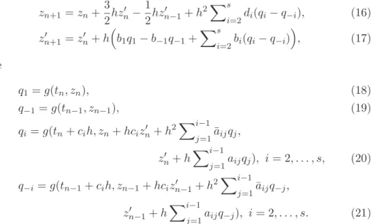
zn+1 =zn+
3 2hz
′
n−
1 2hz
′
n−1+h2
Xs
i=2di(qi−q−i), (16)
z′n+1 =z′n+hb1q1−b−1q−1+
Xs
i=2bi(qi−q−i)
, (17)
where
q1=g(tn, zn), (18)
q−1=g(tn−1, zn−1), (19)
qi=g(tn+cih, zn+hcizn′ +h2Xi−1 j=1¯aijqj,
zn′ +hXi−1
j=1aijqj), i= 2, . . . , s, (20)
q−i=g(tn−1+cih, zn−1+hcizn′−1+h2
Xi−1
j=1a¯ijq−j,
zn′−1+hXi−1
j=1aijq−j), i= 2, . . . , s. (21)
IRKNG method (16)-(21) is expressed using the following Butcher table (see Table 1).
c A¯ A
bT dT
Table 1: The IRKNG Method
3. Order conditions for IRKNG method
Taylor series expansion is used to expand the IRKNG method (16)-(21) to get their parameters. After implementing some algebraic simplifications this extension equal to the real solution. Consequently, a nonlinear equations (called the order conditions) have found using Maple algebra package.
The Taylor series expansion of z(tn+h) and z′(tn+h) for the method
zn+1 =z(tn+h) =z(tn) +hz′(tn) + h2
2 z
′′(t
n) + h3
6 z
′′′(t
n)
+h
4
24z
(iv)(t
n) +. . .+O(hp+1), (22)
zn′+1=z′(tn+h) =z′(tn) +hz′′(tn) + h2
2 z
′′′(t
n) + h3
6 z
(iv)(t
n)
+ h
4
24z
(v)(t
n) +. . .+O(hp+1). (23)
Therefore, the algebraic order conditions of s-stage IRKNG formula up to
fourth order can be given below.
For z:
order three: Xs
i=2di=
5
12, (24)
order four: Xs
i=2dici =
1
6. (25)
For z′:
order one: b1−b−1 = 1, (26)
order two: b−1+
Xs
i=2bi=
1
2, (27)
order three: Xs
i=2bici=
5
12, (28)
Xs
i=2
Xi−1
j=1biaaij =
5
12, (29)
order four: Xs
i=2bic 2
i =
1
3, (30)
Xs
i=3
Xi−1
j=2biaaijcj =
1
6, (31)
Xs
i=2
Xi−1
j=1biaij =
1
6, (32)
1 2
Xs
i=2
Xi−1
j=1biaa 2
ij +
Xs
i=3
Xi−2
j=1
Xi−1
k=2biaaijaaik=
1
6, (33)
Xs
i=2
Xi−1
j=1biciaaij =
1
4. Construction of the newly IRKNG method
We proceed to derive two-stage IRKNG method of order three, denoted as IRKNG3. The following simplifying conditions are used
Xs
j=1aaij =ci,
Xs
j=1aij =
1 2c
2
i. (35)
From (35) we have
aa21=c2, a21=
1 2c
2
2. (36)
The order conditions of IRKNG3 method must satisfy the following equations
d2 =
5
12, (37)
b1−b−1= 1, (38)
b−1+b2 =
1
2, (39)
b2c2 =
5
12. (40)
Solving equations (38) to (40) simultaneously yields a solution depend on c2
as follows:
b−1 =
6c2−5
12c2
, (41)
b1 =
18c2−5
12c2
, (42)
b2 =
5 12c2
. (43)
The global truncation error for the fourth order IRKNG3 formula is given by
kτg(4)k2 =
r
Xnp+1
i=1
τi(4)2+Xnp+1
i=1
τi′(4)2,
whereτ(4) and τ′(4) are the truncation error of z and z′, respectively. Hence,
we have
kτg(4)k2 =
1 24
q 225c2
By using the Minimize command in optimization package in Maple software,
we obtain c2= 35, which gives
kτg(4)k2 = 1.242259987499×10⁻¹,
b−1 =− 7
36,
b1 =
29 36,
b2 =
25 36.
Finally, the parameters of IRKNG method of two-stage third-order indicated by IRKNG3 can be written as follows (see Table 2).
0 0 0
3
5 509 0 35 0
−367 2936 2536 125
Table 2: The IRKNG3 Method
5. Problems tested
Some problems are solved to show the efficiency of IRKNG method in this section. We are comparing the numerical result with the currently RKN and RK formulas. In the comparison we have chosen the following methods:
• IRKNG3: the new two-stage IRKNG method of third-order constructed
in this paper.
• RKN3C: the RKN method of third-order with three-stage given by Chawla
et al. [6].
• RK3B: the RK method of third-order with three-stage given by Butcher
[4].
• IRK3F: the third order IRK method with three-stage derived by Rabiei
Problem 1. ([16])
z′′=−1
xz
′
−(t
2−0.025)
t2 z,
z(1) =
r 2
π sin(1)≃0.6713967061418031,
z′(1) = (2 cos(1)−sin(1))/√2π ≃0.0954005144474746.
The exact solution is
z(t) =J1/2(t) =
r 2
πt sin(t), 1≤t≤6.
RK3B IRK3F RKN3C IRKNG3
log10(Function Evaluations)
lo
g10
(M
G
E
)
4 3.8 3.6 3.4 3.2 3 2.8 2.6 2.4 2.2 -4
-5
-6
-7
-8
-9
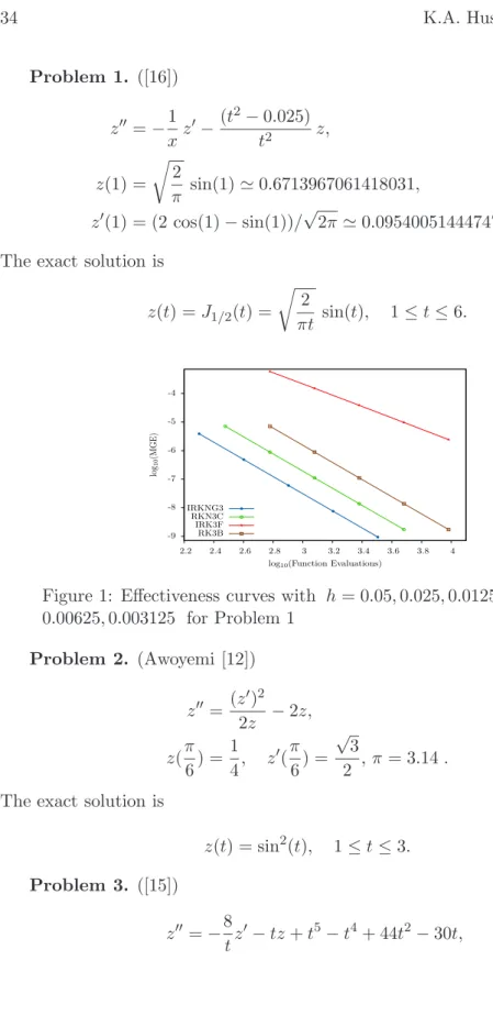
Figure 1: Effectiveness curves with h= 0.05,0.025,0.0125,
0.00625,0.003125 for Problem 1
Problem 2. (Awoyemi [12])
z′′= (z
′)2
2z −2z,
z(π
6) =
1
4, z
′(π
6) =
√
3
2 , π= 3.14.
The exact solution is
z(t) = sin2(t), 1≤t≤3.
Problem 3. ([15])
z′′=−8
tz
′
RK3B IRK3F RKN3C IRKNG3
log10(Function Evaluations)
lo
g10
(M
G
E
)
3.4 3.2 3 2.8 2.6 2.4 2.2 2 1.8 1.6 -1.5
-2
-2.5
-3
-3.5
-4
-4.5
-5
-5.5
-6
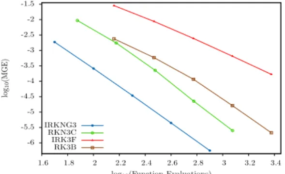
Figure 2: Effectiveness curves with h= 0.1,0.05,0.025,
0.0125,0.00625 for Problem 2
z(1) = 0, z′(1) = 1.
The exact solution is
z(t) =t4−t3, 1≤t≤10.
RK3B IRK3F RKN3C IRKNG3
log10(Function Evaluations)
lo
g10
(M
G
E
)
4 3.8 3.6 3.4 3.2 3 2.8 2.6 2.4 2.2 -1
-2
-3
-4
-5
-6
Figure 3: Effectiveness curves with h= 0.1,0.05,0.025,
0.0125,0.00625 for Problem 3
Problem 4. (Franco [9])
z′′ =−ω2z−δz′, z(0) = 1, z′(0) =−δ/2.
The exact solution is
RK3B IRK3F RKN3C IRKNG3
log10(Function Evaluations)
lo
g10
(M
G
E
)
3.6 3.4 3.2 3 2.8 2.6 2.4 2.2 2 1.8 -1
-1.5
-2
-2.5
-3
-3.5
-4
-4.5
-5
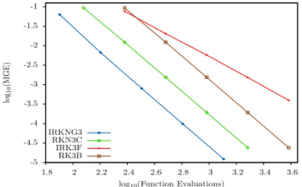
Figure 4: Effectiveness curves with ω= 1, δ = 10−6,
h= 0.5,0.25,0.125,0.0625,0.03125 for Problem 4
From Figures 1 to 4, we observed that IRKNG3 performs better efficiency than the existing RKN3C, RK3B and IRK3F methods of the same order.
6. Conclusion
A new third order two stage IRKNG3 method for direct solution of general second-order ODEs has constructed. The order conditions for IRKNG3 method are derived by using the approach of Taylor series expansion. From Numerical results given in all figures, we observed that the IRKNG3 method is better than the existing methods in terms of maximum error and number of function evaluations.
References
[1] E. Hairer, S.P. Nørsett, G. Wanner, Solving Ordinary Differential
Equa-tions I: Nonstiff Problems, Springer, Berlin (1993).
[2] P.R. Holland, The Quantum Theory of Motion, Cambridge University
Press, Cambridge (2000).
[3] V.A. Avdyushev, Special perturbation theory methods in celestial mechan-ics, I. Principles for the construction and substantiation of the application,
Russian Phys. J.,49 (2006), 1344-1253.
[4] J.C. Butcher,Numerical Methods for Ordinary Differential Equations, 2nd
[5] E. Hairer, G. Wanner, A theory for Nystr¨om methods, Numer. Math. 25
(1976), 383-400.
[6] M.M. Chawla, S.R. Sharma, Families of three-stage third order
Runge Kutta Nystr¨om methods for y′′ =f(x, y, y′), J. Aust. Math. Soc.,
26(1985), 375-386.
[7] B.P. Sommeijer, Explicit, high-order Runge Kutta Nystr¨om methods for
parallel computers, Appl. Numer. Math.,13(1993), 221-240.
[8] E. Hairer, M´ethodes de Nystr¨om pour l’´equation diff´erentielley′′=f(x, y), Numer. Math.,27(1976), 283-300.
[9] J.M. Franco, Exponentially fitted symplectic integrators of RKN type for
solving oscillatory problems,Comput. Phys. Comm.,177(2007), 479-492.
[10] H. Yang, X. Wu, X. You, Y. Fang, Extended RKN-type methods for
nu-merical integration of perturbed oscillators, Comput. Phys. Comm., 180
(2009), 1777-1794.
[11] X. You, J. Zhao, H. Yang, Y. Fang, X. Wu, Order conditions for RKN
methods solving general second-order oscillatory systems, Numer. Algor.,
66(2014), 147-176.
[12] D.O. Awoyemi, A new sixth-order algorithm for general second order
ordi-nary differential equation, International Journal of Computer
Mathemat-ics,77(2001), 117-124.
[13] F. Rabiei, F. Ismail, N. Senu, N. Abasi, Construction of Improved
Runge-Kutta Nystr¨om method for solving second-order ordinary differential
equa-tions,World Applied Sciences Journal,20(2012), 1685-1695.
[14] F. Rabiei, F. Ismail, Third-order Improved Runge-Kutta method for
solv-ing ordinary differential equation,International Journal of Applied Physics
and Mathematics,1 (2011), 191-194.
[15] O. Abu Arqub, A. El-Ajou, A.S. Bataineh, I. Hashim, A Representation of the exact solution of generalized Lane-Emden equations using a new
analytical method,Abstract and Applied Analysis,2013 (2013), 1-10.
[16] J. Vigo-Aguiara, H. Ramos, Variable stepsize implementation of
multi-step methods for y′′ =f(x, y, y′), Journal of Computational and Applied