Getting Data into R
In the following chapter we address entering data into R and organising it as scalars (single values), vectors, matrices, data frames, or lists. We also demon-strate importing data from Excel, ascii files, databases, and other statistical programs.
2.1 First Steps in R
2.1.1 Typing in Small Datasets
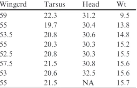
We begin by working with an amount of data that is small enough to type into R. We use a dataset (unpublished data, Chris Elphick, University of Connecti-cut) containing seven body measurements taken from approximately 1100 saltmarsh sharp-tailed sparrows (Ammodramus caudacutus) (e.g., size of the head and wings, tarsus length, weight, etc.). For our purposes we use only four morphometric variables of eight birds (Table 2.1).
The simplest, albeit laborious, method of entering the data into R is to type it in as scalars (variables containing a single value). For the first five observations of wing length, we could type:
Table 2.1 Morphometric measurements of eight birds. The symbolNAstands for a missing value. The measured variables are the lengths of the wing (measured as the wing chord), leg (a standard measure of the tarsus), head (from the bill tip to the back of the skull), and weight.
Wingcrd Tarsus Head Wt 59 22.3 31.2 9.5 55 19.7 30.4 13.8 53.5 20.8 30.6 14.8 55 20.3 30.3 15.2 52.5 20.8 30.3 15.5 57.5 21.5 30.8 15.6 53 20.6 32.5 15.6
55 21.5 NA 15.7
A.F. Zuur et al.,A Beginner’s Guide to R, Use R,
DOI 10.1007/978-0-387-93837-0_2,ÓSpringer ScienceþBusiness Media, LLC 2009 29
> a <- 59 > b <- 55 > c <- 53.5 > d <- 55 > e <- 52.5
Alternatively, you can use the ‘‘=’’ symbol instead of ‘‘<–’’. If you type these commands into a text editor, then copy and paste them into R, nothing appears to happen. To see R’s calculations, type ‘‘a’’ and click enter.
> a
[1] 59
Hence, ‘‘a’’ has the value of 59, as we intended. The problem with this approach is that we have a large amount of data and will quickly run out of characters. Furthermore, the variable names a, b, c, and so on are not very useful as aids for recalling what they represent. We could use variable names such as > Wing1 <- 59
> Wing2 <- 55 > Wing3 <- 53.5 > Wing4 <- 55 > Wing5 <- 52.5
More names will be needed for the remaining data. Before we improve the naming process of the variables, we discuss what you can do with them. Once we have defined a variable and given it a value, we can do calculations with it; for example, the following lines contain valid commands.
> sqrt(Wing1)
> 2 * Wing1
> Wing1 + Wing2
> Wing1 + Wing2 + Wing3 + Wing4 + Wing5
> (Wing1 + Wing2 + Wing3 + Wing4 + Wing5) / 5
Although R performs the calculations, it does not store the results. It is perhaps better to define new variables:
> SQ.wing1 <- sqrt(Wing1)
> Mul.W1 <- 2 * Wing1
> Sum.12 <- Wing1 + Wing2
> SUM12345 <- Wing1 + Wing2 + Wing3 + Wing4 + Wing5
> Av <- (Wing1 + Wing2 + Wing3 + Wing4 + Wing5) / 5
These five lines are used to demonstrate that you can use any name. Note that the dot is a component of the name. We advise the use of variable names that aid in remembering what they represent. For example,SQ.wing1reminds
us that it is the square root of the wing length for bird 1. Sometimes, a bit of imagination is needed in choosing variable names. However, you should avoid names that contain characters like ‘‘£, $, %,^*, +,, ( ), [ ], #, !, ?, <, >, and so on, as most of these characters are operators, for example, multiplication, power, and so on.
As we already explained above, if you have defined
> SQ.wing1 <- sqrt(Wing1)
to display the value ofSQ.wing1, you need to type: > SQ.wing1
[1] 7.681146
An alternative is to put round brackets around the command; R will now produce the resulting value:
> (SQ.wing1 <- sqrt(Wing1))
[1] 7.681146
2.1.2 Concatenating Data with the
c
Function
As mentioned above, with eight observations of four morphometric variables, we need 32 variable names. R allows the storage of multiple values within a variable. For this we need thec()function, where c stands for concatenate. It is used as follows.
> Wingcrd <- c(59, 55, 53.5, 55, 52.5, 57.5, 53, 55)
You may put spaces on either side of the commas to improve the readability of the code. Spaces can also be used on either side of the ‘‘+’’ and ‘‘<-’’ commands. In general, this improves readability of the code, and is recommended.
It is important to use the round brackets ( and ) in thecfunction and not the square [ and ] or the curly brackets { and }. These are used for other purposes. Just as before, copying and pasting the above command into R only assigns the data to the variableWingcrd. To see the data, typeWingcrdinto R and press enter: > Wingcrd
[1] 59.0 55.0 53.5 55.0 52.5 57.5 53.0 55.0
Thecfunction has created a single vector of length 8. To view the first value ofWingcrd, typeWingcrd[1] and press enter:
> Wingcrd [1]
[1] 59
This gives the value 59. To view the first five values type:
> Wingcrd [1 : 5]
[1] 59.0 55.0 53.5 55.0 52.5 To view all except the second value, type:
> Wingcrd [-2]
[1] 59.0 53.5 55.0 52.5 57.5 53.0 55.0
Hence, the minus sign omits a value. R has many built-in functions, the most elementary of which are functions such assum,mean,max,min,median,var, and sd, among othersn. They can be applied by typing
> sum(Wingcrd)
[1] 440.5
Obviously, we can also store the sum in a new variable
> S.win <- sum(Wingcrd)
> S.win
[1] 440.5
Again, the dot is part of the variable name. Now, enter the data for the other three variables from Table 2.1 into R. It is laborious, but typing the following code into an editor, then copying and pasting it into R does the job.
> Tarsus <- c(22.3, 19.7, 20.8, 20.3, 20.8, 21.5, 20.6,
21.5)
> Head <- c(31.2, 30.4, 30.6, 30.3, 30.3, 30.8, 32.5,
NA)
> Wt <- c(9.5, 13.8, 14.8, 15.2, 15.5, 15.6, 15.6,
15.7)
Note that we are paying a price for the extra spaces; each command now extends into two lines. As long as you end the line with a backslash or a comma, R will consider it as one command.
It may be a good convention to capitalize variable names. This avoids confusion with existing function commands. For example, ‘‘head’’ is an exist-ing function in R (see ?head). Most internal functions do not begin with a capital letter; hence we can be reasonably sure thatHead is not an existing function. If you are not completely sure, try typing, for example,?Head. If a help file pops up, you know that you need to come up with another variable name.
Note that there is one bird for which the size of the head was not measured. It is indicated byNA. Depending on the function, the presence of anNAmay, or may not, cause trouble. For example:
> sum(Head)
[1] NA
You will get the same result with the mean, min, max, and many other functions. To understand why we getNAfor the sum of the head values, type ?sum. The following is relevant text from thesumhelp file.
...
sum(..., na.rm = FALSE) ...
If na.rm is FALSE, an NA value in any of the arguments will cause a value of NA to be returned, otherwise NA values are ignored.
...
Apparently, the default ‘‘na.rm =FALSE’’ option causes the R function sumto return an NA if there is a missing value in the vector (rm refers to remove). To avoid this, use ‘‘na.rm=TRUE’’
> sum(Head, na.rm = TRUE)
[1] 216.1
Now, the sum of the seven values is returned. The same can be done for the mean,min,max, andmedianfunctions. On most computers, you can also use na.rm=Tinstead ofna.rm=TRUE. However, because we have been con-fronted with classroom PCs running identical R versions on the same operating system, and a few computers give an error message with thena.rm=Toption, we advise usingna.rm=TRUE.
You should always read the help file for any function before use to ensure that you know how it deals with missing values. Some functions usena.rm, some use na.action, and yet others use a different syntax. It is nearly impossible to memorise how all functions treat missing values.
Summarising, we have entered data for four variables, and have applied simple functions such asmean,min,max, and so on.We now discuss methods of combining the data of these four variables: (1) thec,cbind, and rbind functions; (2) the matrix and vector functions; (3) data frames; and (4) lists.
2.1.3 Combining Variables with the
c
,
cbind
, and
rbind
Functions
We have four columns of data, each containing observations of eight birds. The variables are labelledWingcrd,Tarsus,Head,andWt. Thecfunction was used to concatenate the eight values. In the same way as the eight values were concatenated, so can we concatenate the variables containing the values using:
> BirdData <- c(Wingcrd, Tarsus, Head, Wt)
Our use of the variable nameBirdDatainstead ofdata, means that we are not overwriting an existing R function (see?data). To see the result of this command, typeBirdDataand press enter:
> BirdData
[1] 59.0 55.0 53.5 55.0 52.5 57.5 53.0 55.0 22.3
[10] 19.7 20.8 20.3 20.8 21.5 20.6 21.5 31.2 30.4
[19] 30.6 30.3 30.3 30.8 32.5 NA 9.5 13.8 14.8
[28] 15.2 15.5 15.6 15.6 15.7
BirdData is a single vector of length 32 (48). The numbers [1], [10], [19], and [28] are the index numbers of the first element on a new line. On your computer they may be different due to a different screen size. There is no need to pay any attention to these numbers yet.
R produces all 32 observations, including the missing value, as a single vector, because it does not distinguish values of the different variables (the first 8 observations are of the variable Wingcrd, the second 8 from Tarsus, etc.) . To counteract this we can make a vector of length 32, call it Id (for ‘‘identity’’), and give it the following values.
> Id <- c(1, 1, 1, 1, 1, 1, 1, 1, 2, 2, 2, 2, 2, 2, 2,
2, 3, 3, 3, 3, 3, 3, 3, 3, 4, 4, 4, 4, 4, 4, 4, 4) > Id
[1] 1 1 1 1 1 1 1 1 2 2 2 2 2 2 2 2 3 3 3 3 3 3 3
[24] 3 4 4 4 4 4 4 4 4
Because R can now put more digits on a line, as compared to inBirdData, only the indices [1] and [24] are produced. These indices are completely irrele-vant for the moment. The variableIdcan be used to indicate that all observa-tions with a similar Id value belong to the same morphometric variable. However, creating such a vector is time consuming for larger datasets, and, fortunately, R has functions to simplify this process. What we need is a function that repeats the values 1 –4, each eight times:
> Id <- rep(c(1, 2, 3, 4), each = 8) > Id
[1] 1 1 1 1 1 1 1 1 2 2 2 2 2 2 2 2 3 3 3 3 3 3 3
[24] 3 4 4 4 4 4 4 4 4
This produces the same long vector of numbers as above. Therep designa-tion stands for repeat. The command can be further simplified by using:
> Id <- rep(1 : 4, each = 8)
> Id
[1] 1 1 1 1 1 1 1 1 2 2 2 2 2 2 2 2 3 3 3 3 3 3 3
[24] 3 4 4 4 4 4 4 4 4
Again, we get the same result. To see what the1 : 4command does, type into R:
> 1 : 4
It gives
[1] 1 2 3 4
So the : operator does not indicate division (as is the case with some other packages). You can also use theseqfunction for this purpose. For example, the command
> a <- seq(from = 1, to = 4, by = 1)
> a
creates the same sequence from 1 to 4,
[1] 1 2 3 4
So for the bird data, we could also use:
> a <- seq(from = 1, to = 4, by = 1)
> rep(a, each = 8)
[1] 1 1 1 1 1 1 1 1 2 2 2 2 2 2 2 2 3 3 3 3 3 3 3
[24] 3 4 4 4 4 4 4 4 4
Each of the digits in ‘‘a’’ is repeated eight times by therepfunction. At this stage you may well be of the opinion that in considering so many different options we are making things needlessly complicated. However, some functions in R need the data as presented in Table 2.1 (e.g, the multivariate analysis function for principal component analysis or multidimensional scaling), whereas the organisation of data into a single long vector, with an extra variable to identify the groups of observations (Id in this case), is needed for other functions such as thet-test, one-way anova, linear regression, and also for some graphing tools such as thexyplotin thelatticepackage (see Chapter 8). Therefore, fluency with therepfunction can save a lot of time.
So far, we have only concatenated numbers. But suppose we want to create a vector ‘‘Id’’ of length 32 that contains the word ‘‘Wingcrd’’ 8 times, the word ‘‘Tarsus’’ 8 times, and so on.We can create a new variable calledVarNames, containing the four morphometric variable designations. Once we have created it, we use therepfunction to create the requested vector:
> VarNames <- c("Wingcrd", "Tarsus", "Head", "Wt") > VarNames
[1] "Wingcrd" "Tarsus" "Head" "Wt"
Note that these are names, not the variables with the data values. Finally, we need:
> Id2 <- rep(VarNames, each = 8)
> Id2
[1] "Wingcrd" "Wingcrd" "Wingcrd" "Wingcrd"
[5] "Wingcrd" "Wingcrd" "Wingcrd" "Wingcrd"
[9] "Tarsus" "Tarsus" "Tarsus" "Tarsus"
[13] "Tarsus" "Tarsus" "Tarsus" "Tarsus"
[17] "Head" "Head" "Head" "Head"
[21] "Head" "Head" "Head" "Head"
[25] "Wt" "Wt" "Wt" "Wt"
[29] "Wt" "Wt" "Wt" "Wt"
Id2is a string of characters with the names in the requested order. The difference between Id and Id2 is just a matter of labelling. Note that you should not forget the "each=" notation. To see what happens if it is omitted, try typing:
> rep(VarNames, 8)
[1] "Wingcrd" "Tarsus" "Head" "Wt"
[5] "Wingcrd" "Tarsus" "Head" "Wt"
[9] "Wingcrd" "Tarsus" "Head" "Wt"
[13] "Wingcrd" "Tarsus" "Head" "Wt"
[17] "Wingcrd" "Tarsus" "Head" "Wt"
[21] "Wingcrd" "Tarsus" "Head" "Wt"
[25] "Wingcrd" "Tarsus" "Head" "Wt"
[29] "Wingcrd" "Tarsus" "Head" "Wt"
It will produce a repetition of the entire vector VarNames with the four variable names listed eight times, not what we want in this case.
Thecfunction is a way of combining data or variables. Another option is the cbind function. It combines the variables in such a way that the output contains the original variables in columns. For example, the output of the cbindfunction below is stored inZ. If we typeZand press enter, it shows the values in columns:
> Z <- cbind(Wingcrd, Tarsus, Head, Wt) > Z
Wingcrd Tarsus Head Wt
[1,] 59.0 22.3 31.2 9.5
[2,] 55.0 19.7 30.4 13.8
[3,] 53.5 20.8 30.6 14.8
[4,] 55.0 20.3 30.3 15.2
[5,] 52.5 20.8 30.3 15.5
[6,] 57.5 21.5 30.8 15.6
[7,] 53.0 20.6 32.5 15.6
[8,] 55.0 21.5 NA 15.7
The data must be in this format if we are to apply, for example, principal component analysis. Suppose you want to access some elements of Z, for instance, the data in the first column. This is done with the commandZ [, 1]:
> Z[, 1]
[1] 59.0 55.0 53.5 55.0 52.5 57.5 53.0 55.0
Alternatively, use
> Z[1 : 8, 1]
[1] 59.0 55.0 53.5 55.0 52.5 57.5 53.0 55.0
It gives the same result. The second row is given byZ [2,]:
> Z[2, ]
Wingcrd Tarsus Head Wt
55.0 19.7 30.4 13.8
Alternatively, you can use:
> Z[2, 1:4]
Wingcrd Tarsus Head Wt
55.0 19.7 30.4 13.8
The following commands are all valid.
> Z[1, 1]
> Z[, 2 : 3]
> X <- Z[4, 4] > Y <- Z[, 4] > W <- Z[, -3]
> D <- Z[, c(1, 3, 4)]
> E <- Z[, c(-1, -3)]
The first command accesses the value of the first bird for Wingcrd; the second command gives all the data for columns 2 and 3;Xcontains the weight for bird 4; andY,all theWtdata. The minus sign is used to exclude columns or rows. Hence,Wcontains all variables exceptHead. We can also use thecfunction
to access nonsequential rows or columns ofZ.Dcontains the first, third, and fourth columns ofZ, andEcontains all but the first and third. You must ensure that the subscripts do not go outside the range of allowable values. For example,Z [8, 4]is valid, butZ [9, 5],Z [8, 6], orZ [10, 20]are not defined (we only have 8 birds and 4 variables). If you type one of these commands, R will give the error message: Error: subscript out of bounds
If you would like to know the dimensions ofZ, use: > dim(Z)
[1] 8 4
The output is a vector with two elements: the number of rows and the number of columns ofZ. At this point you may want to consult the help files ofnrowandncolfor alternative options. In some situations, it may be useful to store the output of thedimfunction. In that case, use
> n <- dim(Z) > n
[1] 8 4
or, if you only need to store the number of rows inZ, use
> nrow <- dim(Z)[1]
> nrow
[1] 8
Instead ofnrow, the variable namezrowmay be more appropriate. As you would expect, similar to thecbind function to arrange the variables in col-umns, therbindfunction combines the data in rows. To use it, type:
> Z2 <- rbind(Wingcrd, Tarsus, Head, Wt)
> Z2
[,1] [,2] [,3] [,4] [,5] [,6] [,7] [,8]
Wingcrd 59.0 55.0 53.5 55.0 52.5 57.5 53.0 55.0
Tarsus 22.3 19.7 20.8 20.3 20.8 21.5 20.6 21.5
Head 31.2 30.4 30.6 30.3 30.3 30.8 32.5 NA
Wt 9.5 13.8 14.8 15.2 15.5 15.6 15.6 15.7
This gives the same data as in the previous examples, with the morphometric variables in rows and the individual birds in columns.
Other interesting tools to changeZorZ2are theeditandfixfunctions; see their help files.
Do Exercise 2 in Section 2.4 in the use of thecandcbind func-tions. This is an exercise using an epidemiological dataset.
2.1.4 Combining Data with the
vector
Function*
To avoid introducing too much information, we did not mention thevector function in the previous discussion, and upon first reading, you may skip this section. Instead of thecfunction, we could have used thevector function. Suppose we want to create a vector of length 8 containing dataWingcrdof all eight birds. In R, we can do this as follows.
> W <- vector(length = 8)
> W[1] <- 59 > W[2] <- 55 > W[3] <- 53.5 > W[4] <- 55 > W[5] <- 52.5 > W[6] <- 57.5 > W[7] <- 53 > W[8] <- 55
If you typeWinto R immediately after the first command, R shows a vector with values FALSE. This is normal. TypingWinto R after all elements have been entered gives:
> W
[1] 59.0 55.0 53.5 55.0 52.5 57.5 53.0 55.0
Note that the result is identical to that of thecfunction. The advantage of the vector function is that we can define a priori how many elements a variable should have. This can be useful when doing specific tasks such as loops. However, for common applications, it is easier to use thecfunction to concatenate data.
Just as with the output of thecfunction, we can access particular elements of WusingW [1],W [1 : 4],W [2 : 6],W [-2],W [c (1, 3, 5)], butW [9]produces an NA, as element 9 is not defined.
Do Exercise 3 in Section 2.4 in the use of thevectorfunction. This is an exercise using an epidemiological dataset.
2.1.5 Combining Data Using a Matrix*
Upon first reading, you may skip this section.Instead of vectors showing the 4 variablesWingcrd,Tarsus,Head, and Wt, each of length 8, we can create a matrix of dimension 8 by 4 that contains the data. Such a matrix is created by the command:
> Dmat <- matrix(nrow = 8, ncol = 4) > Dmat
[,1] [,2] [,3] [,4]
[1,] NA NA NA NA
[2,] NA NA NA NA
[3,] NA NA NA NA
[4,] NA NA NA NA
[5,] NA NA NA NA
[6,] NA NA NA NA
[7,] NA NA NA NA
[8,] NA NA NA NA
We first wanted to call this matrixD, but subsequently discovered that Tinn-R uses a blue font forD, meaning that it is an existing function. Entering?D gives the information that it is a function to calculate derivates, hence we will not overwrite it. We instead use the designator ‘‘Dmat,’’ where ‘‘mat’’ indicates matrix.
Note thatDmatis an 8 by 4 matrix containing only NAs. We need to fill in the values. This can be done by
> Dmat[, 1] <- c(59, 55, 53.5, 55, 52.5, 57.5, 53, 55)
> Dmat[, 2] <- c(22.3, 19.7, 20.8, 20.3, 20.8, 21.5,
20.6, 21.5)
> Dmat[, 3] <- c(31.2, 30.4, 30.6, 30.3, 30.3, 30.8,
32.5, NA)
> Dmat[, 4] <- c(9.5, 13.8, 14.8, 15.2, 15.5, 15.6,
15.6, 15.7)
The elements ofDmat, in this case,are entered by column, but we could have filled them in by row. Typing Dmatinto R gives the same data matrix as we obtained with thecbindfunction, except thatDmatdoes not have column labels:
> Dmat
[,1] [,2] [,3] [,4]
[1,] 59.0 22.3 31.2 9.5
[2,] 55.0 19.7 30.4 13.8
[3,] 53.5 20.8 30.6 14.8
[4,] 55.0 20.3 30.3 15.2
[5,] 52.5 20.8 30.3 15.5
[6,] 57.5 21.5 30.8 15.6
[7,] 53.0 20.6 32.5 15.6
We can use the existingcolnamesfunction to add column names toDmat: > colnames(Dmat) <- c("Wingcrd", "Tarsus", "Head","Wt") > Dmat
Wingcrd Tarsus Head Wt
[1,] 59.0 22.3 31.2 9.5
[2,] 55.0 19.7 30.4 13.8
[3,] 53.5 20.8 30.6 14.8
[4,] 55.0 20.3 30.3 15.2
[5,] 52.5 20.8 30.3 15.5
[6,] 57.5 21.5 30.8 15.6
[7,] 53.0 20.6 32.5 15.6
[8,] 55.0 21.5 NA 15.7
Obviously, there is also arownamesfunction, the use of which is explained in the help file.
To summarise, we first defined a matrix of a specific size, then filled in its elements by column. You must define the matrix before you enter its elements. You can also fill in element by element, for example,
> Dmat[1, 1] <- 59.0
> Dmat[1, 2] <- 22.3
and so on, but this takes more time. If we have the data already categorized in variables, such asWingcrd,Tarsus,Head,Wt, we would not normally create the matrix and fill in its elements. This command will do the job as well:
> Dmat2 <- as.matrix(cbind(Wingcrd, Tarsus, Head, Wt))
Dmat2andDmatare identical. Once again learning more than one path to the same outcome is necessary because some functions require a matrix as input and will give an error message if a data frame (see next subsection) is used, and vice versa. Therefore, functions such asas.matrix,is.matrix(this function gives a
TRUEif its argument is a matrix, andFALSEotherwise),as.data.frame,is. date.framecan come in handy.
Special operators for matricesAandBaret(A) for transpose,A%*%Bfor matrix multiplication, andsolve (A)for inverse.
2.1.6 Combining Data with the
data.frame
Function
So far, we have used thec,cbind,rbind,vector, andmatrixfunctions to combine data. Yet another option is the data frame. In a data frame we can combine variables of equal length, with each row in the data frame containing observations on the same sampling unit. Hence, it is similar to thematrixor cbind functions. Using the four bird morphometric variables from the pre-vious section, a data frame is created as follows.
> Dfrm <- data.frame(WC = Wingcrd,
TS = Tarsus, HD = Head,
W = Wt) > Dfrm
WC TS HD W
1 59.0 22.3 31.2 9.5
2 55.0 19.7 30.4 13.8 3 53.5 20.8 30.6 14.8 4 55.0 20.3 30.3 15.2 5 52.5 20.8 30.3 15.5 6 57.5 21.5 30.8 15.6 7 53.0 20.6 32.5 15.6
8 55.0 21.5 NA 15.7
Basically, thedata.framefunction creates an object, calledDfrmin this case, and withinDfrmit stores values of the four morphometric variables. The advan-tage of a data frame is that you can make changes to the data without affecting the original data. For example, it is possible to combine the original (but renamed) weight and the square root transformed weights in the data frameDfrm:
> Dfrm <- data.frame(WC = Wingcrd,
TS = Tarsus, HD = Head,
W = Wt
Wsq = sqrt(Wt))
In the data frame, we can also combine numerical variables, character strings, and factors. Factors are nominal (categorical) variables and are dis-cussed later in this chapter.
It is important to realise that the variableWtthat we created in thecfunction and theWin the data frameDfrmare two different entities. To see this, let us remove the variableWt(this is the one we typed in with thecfunction): > rm(Wt)
> Wt
Error: object "Wt" not found
But the variable W still exists in the data frame Dfrm:
> Dfrm$W
[1] 9.5 13.8 14.8 15.2 15.5 15.6 15.6 15.7
It may seem that the data frame is unnecessary, because we have the cbin-dandmatrix functions, However, neither of these can be used to combine different types of data. Our use of the data frame is often as follows. First we enter the data into R, mainly using methods discussed in Section 2.2. We then make changes to the data (e.g., remove extreme observations, apply transfor-mations, add categorical variables, etc.) and store the modified data in a data frame which we use in the follow-up analyses.
2.1.7 Combining Data Using the
list
Function*
You may also skip this section at first reading. So far, the tools we have used to combine data produce a table with each row being a sampling unit (a bird in this case). Suppose you want a black box into which you can put as many variables as you want; some may be related, some may have similar dimen-sions, some may be vectors, others matrices, and yet others may contain character strings of variable names. This is what the listfunction can do. The main difference from our previously used methods is that the resulting rows will not necessarily represent a single sampling unit. A simple example is given below. The variablesx1,x2,x3, andx4contain data:x1is a vector of length 3,x2contains 4 characters,x3is a variable of dimension 1, andx4is a matrix of dimension 2-by-2. All these variables are entered into the list function:
> x1 <- c(1, 2, 3)
> x2 <- c("a", "b", "c", "d") > x3 <- 3
> x4 <- matrix(nrow = 2, ncol = 2)
> x4[, 1] <- c(1, 2)
> x4[, 2] <- c( 3, 4)
> Y <- list(x1 = x1, x2 = x2, x3 = x3, x4 = x4)
> Y $x1
[1] 1 2 3
$x2
[1] "a" "b" "c" "d"
$x3
[1] 3
$x4
[,1] [,2]
[1,] 1 3
[2,] 2 4
All information contained inYis accessible by typing, for example,Y$x1, Y$x2, and so on. Again, you may wonder why we need to go to all this trouble. The reason is that nearly all functions (e.g., linear regression, generalised linear modelling,t-test, etc.) in R produce output that is stored in a list. For example, the following code applies a linear regression model in which wing length is modelled as a function of weight.
> M <- lm(WC Wt, data = Dfrm)
We do not wish to go into detail of thelm function, or how to do linear regression in R (see its helpfile obtained by typing?lm). All what we want to emphasise is that R stores all results of the linear regression function in the objectM. If you type
> names(M)
you receive this fancy output:
[1] "coefficients" "residuals" "effects"
[4] "rank" "fitted.values" "assign"
[7] "qr" "df.residual" "xlevels"
[10] "call" "terms" "model"
You can access the coefficients or residuals by using M$coefficients, M$residuals, and so on. Hence, M is a list containing objects of different dimensions, just as our earlier example withY. The good news is that R contains various functions to extract required information (e.g., estimated values,p-values, etc.) and presents it in nice tables. See thelmhelp file.
For the bird morphometric data, it does not make sense to store the data in a list, as the rows in Table 2.1 contain data from thesamebird. However, if the task is to create a list that contains all data in a long vector, an extra vector that identifies the groups of variables (IDin this case), a matrix that contains the data in a 8 by 4 format, and, finally, a vector that contains the 4 morphometric names, we can use:
> AllData <- list(BirdData = BirdData, Id = Id2, Z = Z,
VarNames = VarNames)
to produce: > AllData $BirdData
[1] 59.0 55.0 53.5 55.0 52.5 57.5 53.0 55.0 22.3
[10] 19.7 20.8 20.3 20.8 21.5 20.6 21.5 31.2 30.4
[19] 30.6 30.3 30.3 30.8 32.5 NA 9.5 13.8 14.8
[28] 15.2 15.5 15.6 15.6 15.7
$Id
[1] "Wingcrd" "Wingcrd" "Wingcrd" "Wingcrd"
[5] "Wingcrd" "Wingcrd" "Wingcrd" "Wingcrd"
[9] "Tarsus" "Tarsus" "Tarsus" "Tarsus"
[13] "Tarsus" "Tarsus" "Tarsus" "Tarsus"
[17] "Head" "Head" "Head" "Head"
[21] "Head" "Head" "Head" "Head"
[25] "Wt" "Wt" "Wt" "Wt"
[29] "Wt" "Wt" "Wt" "Wt"
$Z
Wingcrd Tarsus Head Wt
[1,] 59.0 22.3 31.2 9.5
[2,] 55.0 19.7 30.4 13.8
[3,] 53.5 20.8 30.6 14.8
[4,] 55.0 20.3 30.3 15.2
[5,] 52.5 20.8 30.3 15.5
[6,] 57.5 21.5 30.8 15.6
[7,] 53.0 20.6 32.5 15.6
[8,] 55.0 21.5 NA 15.7
$VarNames
[1]"Wingcrd""Tarsus" "Head" "Wt"
Obviously, storing the data in this format is unnecessary, as we only need one format. An advantage, perhaps, with multiple formats, is that we are prepared for most functions. However, our own programming style is such that we only change the format if, and when, needed.
TypingAllDatain R produces the data in most formats that we have seen in this section. It is nice to know that we can do it.
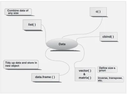
You cannot use the ‘‘<-’’ symbols in thelistfunction, only the ‘‘=’’ sign is accepted. Figure 2.1 shows an overview of the methods of storing data discussed so far.
Do Exercise 5 in Section 2.4. This is an exercise that deals again with an epidemiological dataset and the use of thedata.frame andlistcommands.
2.2 Importing Data
With large datasets, typing them in, as we did in the previous section, is not practical. The most difficult aspect of learning to use a new package is import-ing your data. Once you have mastered this step, you can experiment with other commands. The following sections describe various options for importing data. We make a distinction between small and large datasets and whether they are stored in Excel, ascii text files, a database program, or in another statistical package.
Data
data.frame ( ) list( )
c( )
cbind( )
vector( ) & matrix( )
Combine data of any size
Tidy up data and store in new object
Inverse, transpose, etc.
Define size a
priori
Fig. 2.1 Overview of various methods of storing data. The data stored bycbind,matrix, or data.frameassume that data in each row correspond to the same observation (sample, case)
2.2.1 Importing Excel Data
There are two main options for importing data from Excel (or indeed any spreadsheet or database program) into R. The easy, and recommended, option is (1) to prepare the data in Excel, (2) export it to a tab-delimited ascii file, (3) close Excel, and (4) use theread.tablefunction in R to import the data. Each of these steps is discussed in more detail in the following sections. The second option is a special R package, RODBC, which can access selected rows and columns from an Excel spreadsheet. However, this option is not for the fainthearted. Note that Excel is not particularly suitable for working with large datasets, due to its limitation in the number of columns.
2.2.1.1 Prepare the Data in Excel
In order to keep things simple, we recommend that you arrange the data in a sample-by-variable format. By this, we mean with the columns containing variables, and the rows containing samples, observations, cases, subjects, or whatever you call your sampling units. Enter NA (in capitals) into cells representing missing values. It is good practice to use the first column in Excel for identifying the sampling unit, and the first row for the names of the variables. As mentioned earlier, using names containing symbols such as £, $, %,^, &, *, (, ),, #, ?, , ,. ,<, >, /, |, \, ,[ ,] ,{, and } will result in an error message in R. You should also avoid names (or fields or values) that contain spaces. Short names are advisable in order to avoid graphs containing many long names, making the figure unreadable.
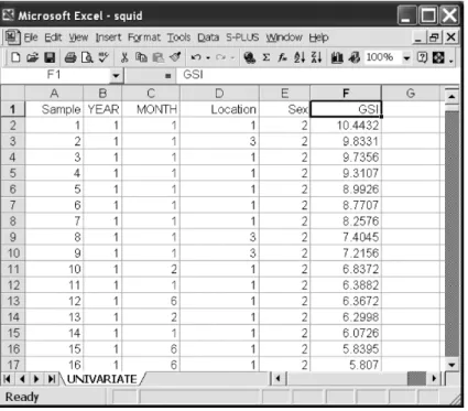
Figure 2.2 shows an Excel spreadsheet containing a set of data on the Gonadosomatic index (GSI, i.e., the weight of the gonads relative to total body weight) of squid (Graham Pierce, University of Aberdeen, UK, unpub-lished data). Measurements were taken from squid caught at various locations in Scottish waters in different months and years.
2.2.1.2 Export Data to a Tab-Delimited ascii File
In Excel, go toFile->Save As->Save as Type, and selectText (Tab delimited). If you have a computer running in a non-English language, it may be a challenge to determine how ‘‘Tab delimited’’ is translated. We exported the squid data in Fig. 2.2 to a tab-delimited ascii file named squid.txt, in the directory C:\RBook. Both the Excel file and the tab-delimited ascii file can be downloaded from the book’s website. If you download them to a different directory, then you will need to adjust the ‘‘C:\RBook’’ path.
At this point it is advisable to close Excel so that it cannot block other programs from accessing your newly created text file.
Warning:Excel has the tendency to add extra columns full of NAs to the ascii file if you have, at some stage, typed comments into the spreadsheet. In R, these columns may appear as NAs. To avoid this, delete such columns in Excel before starting the export process.
2.2.1.3 Using theread.tableFunction
With a tab-delimited ascii file that contains no blank cells or names with spaces, we can now import the data into R. The function that we use isread.table, and its basic use is as follows.
> Squid <- read.table(file = "C:\\RBook\\squid.txt",
header = TRUE)
This command reads the data from the filesquid.txt and stores the data in Squidas a data frame. We highly recommend using short, but clear, variable labels. For example, we would not advise using the name SquidNorthSea-MalesFemales, as you will need to write out this word frequently. A spelling mistake and R will complain. Theheader=TRUEoption in theread.table function tells R that the first row contains labels. If you have a file without headers, change it toheader=FALSEThere is another method of specifying the location of the text file:
> Squid <- read.table(file = "C:/RBook/squid.txt",
header = TRUE)
Fig. 2.2 Example of the organisation of a dataset in Excel prior to importing it into R. The rows contain the cases (each row represents an individual squid) and the columns the vari-ables. The first column and the first row contain labels, there are no labels with spaces, and there are no empty cells in the columns that contain data
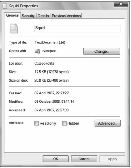
Note the difference in the slashes. If you have error messages at this stage, make sure that the file name and directory path were correctly specified. We strongly advise keeping the directory names simple. We have seen too many people struggling for half an hour to get theread.tablefunction to run when they have a typing error in the 150–200-character long directory structure. In our case, the directory structure is short, C:/RBook. In most cases, the directory path will be longer. It is highly likely that you will make a mistake if you type in the directory path from memory. Instead, you can right-click the file Squid.txt (in Windows Explorer), and click Properties (Fig. 2.3). From here, you can copy and paste the full directory structure (and the file name) into your R text editor. Don’t forget to add the extra slash \.
Fig. 2.3 Properties of the file squid.txt. The file name is Squid.txt, and the location is C:\Bookdata. You can highlight the location, copy it, paste it into theread.tablefunction in your text R editor, and add the extra \ on Windows operating systems
If you use names that include ‘‘My Files,’’ be sure to include the space and the capitals. Another common reason for an error message is the character used for decimal points. By default, R assumes that the data in the ascii text file have point separation, and theread.tablefunction is actually using:
> Squid <- read.table(file = "C:/RBook/squid.txt",
header = TRUE, dec = ".")
If you are using comma separation, change the last option todec = ",", and rerun the command.
Warning:If your computer uses comma separation, and you export the data from Excel to a tab-delimited ascii file, then you must use thedec = ","
option. However, if someone else has created the ascii file using point separa-tion, you must use thedec = "."option. For example, the ascii files for this book are on the book website and were created with point separation. Hence all datasets in this book have to be imported with thedec = "."option, even if your computer uses comma separation. If you use the wrong setting, R will import all numerical data as categorical variables. In the next chapter, we discuss thestrfunction, and recommend that you always execute it immedi-ately after importing the data to verify the format.
If the data have spaces in the variable names, and if you use the read.-table function as specified above, you will get the following message. (We temporarily renamed GSI to G S I in Excel in order to create the error message.)
Error in scan(file,what,nmax,sep,dec,quote,skip,nlines, na.strings,: line 1 did not have 8 elements
R is now complaining about the number of elements per line. The easy option is to remove any spaces from names or data fields in Excel and repeat the steps described above. The same error is obtained if the data contain an empty cell or fields with spaces. Instead of modifying the original Excel file, it is possible to tell theread.tablefunction that there will be fields with spaces. There are many other options for adapting theread.tablefunction to your data. The best way to see them all is to go to theread.tablehelp file. The first part of the help file is shown below. You are not expected to know the meaning of all the options, but it is handy to know that it is possible to change certain settings. read.table(file, header = FALSE, sep = "",
quote = "\"’", dec = ".", row.names, col.names, as.is = !stringsAsFactors,
na.strings = "NA", colClasses = NA, nrows=-1, skip = 0, check.names = TRUE,
strip.white = FALSE, blank.lines.skip = TRUE, comment.char = "#", allowEscapes = FALSE, flush = FALSE,
stringsAsFactors = default.stringsAsFactors())
This is a function with many options. For example if you have white space in the fields, use the optionstrip.white=TRUE. An explanation of the other options can be found under the Arguments section in the help file. The help file also gives information on reading data in csv format. It is helpful to know that the read.tablecan contain an URL link to a text file on an Internet webpage.
If you need to read multiple files from the same directory, it is more efficient (in terms of coding) to set the working directory with thesetwdfunction. You can then omit the directory path in front of the text file in theread.table function. This works as follows.
> setwd("C:\\RBook\\")
> Squid <- read.table(file = "squid.txt", header = TRUE)
In this book, we import all datasets by designating the working directory with thesetwdfunction, followed by theread.tablefunction. Our motiva-tion for this is that not all users of this book may have permission to save files on the C drive (and some computers may not have a C drive!). Hence, they only need to change the directory in thesetwdfunction.
In addition to theread.tablefunction, you can also import data with the scanfunction. The difference is that theread.tablestores the data in a data frame, whereas the scan function stores the data as a matrix. The scan function will work faster (which is handy for large datasets, where large refers to millions of data points), but all the data must be numerical. For small datasets, you will hardly know the difference in terms of computing time. For further details on thescanfunction, see its help file obtained with?scan.
Do Exercises 6 and 7 in Section 2.4 in the use of theread.table andscanfunctions. These exercises use epidemiological and deep sea research data.
2.2.2 Accessing Data from Other Statistical Packages**
In addition to accessing data from an ascii file, R can import data from other statistical packages, for example, Minitab, S-PLUS, SAS, SPSS, Stata, and Systat, among others. However, we stress that it is best to work with the original data directly, rather than importing data possibly modified by another statis-tical software package. You need to type:
in order to access these options. The help file for reading Minitab files is obtained by typing:
> ?read.mtp
and provides a good starting point. There is even awrite.foreignfunction with the syntax:
write.foreign(df, datafile, codefile,
package = c("SPSS", "Stata", "SAS"), ...)
Hence, you can export information created in R to some of the statistical packages. The options in the functionwrite.foreign are discussed in its help file.
2.2.3 Accessing a Database***
This is a rather more technical section, and is only relevant if you want to import data from a database. Accessing or importing data from a database is relatively easy. There is a special package available in R that provides the tools you need to quickly gain access to any type of database. Enter:
> library(RODBC)
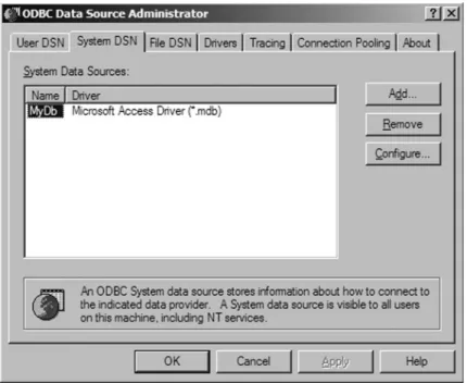
to make the necessary objects available. The package implements Open DataBase Connectivity (ODBC) with compliant databases when drivers exist on the host system. Hence, it is essential that the necessary drivers were set up when installing the database package. In Windows, you can check this through the Administrative Tools menu or look in the Help and Support pages under ODBC. Assuming you have the correct drivers installed, start by setting up a connection to a Microsoft Access database using the odbcConnectAccess: command. Let us call that connection channel1; so type in:
> setwd("C:/RBook")
> channel1 <- odbcConnectAccess(file =
"MyDb.mdb", uid = "", pwd = "")
As you can see, the database, called MyDB.mdb, does not require a user identification (uid) or password (pwd) which, hence, can be omitted. You could have defined a database on your computer through the DSN naming protocol as shown in Fig. 2.4.
Now we can connect to the database directly using the name of the database: > Channel1 <- odbcConnect("MyDb.mdb")
Once we have set up the connection it is easy to access the data in a table: > MyData <- sqlFetch(channel1, "MyTable")
We usesqlFetch to fetch the data and store it in MyData. This is not all you can do with an ODBC connection. It is possible to select only certain rows of the table in the database, and, once you have mastered the necessary database language, to do all kinds of fancy queries and table manipulations from within R. This language, called Structured Query Language, or SQL, is not difficult to learn. The command used in RODBC to send an SQL query to the database is sqlQuery(channel, query) in which query is simply an SQL query between quotes. However, even without learning SQL, there are some commands available that will make working with databases easier. You can usesqlTables to retrieve table information in your database with the command SqlTables(channel) or sqlColumns(chan-nel, "MyTable") to retrieve information in the columns in a database table called MyTable. Other commands aresqlSave, to write or update a table in an ODBC database; sqlDrop, to remove a table; and sqlClear, to delete the content.
Fig. 2.4 Windows Data Source Administrator with the database MyDb added to the system data source names
Windows users can useodbcConnectExcel to connect directly to Excel spreadsheet files and can select rows and columns from any of the sheets in the file. The sheets are represented as different tables.
There are also special packages for interfacing with Oracle (ROracle) and MySQL (RMySQL).
2.3 Which R Functions Did We Learn?
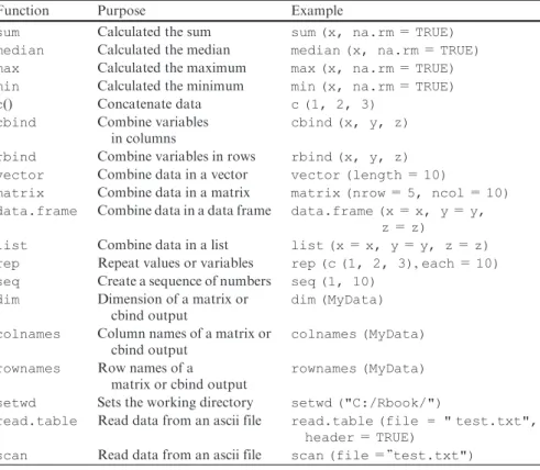
Table 2.2 shows the R functions introduced in this chapter.
2.4 Exercises
Exercise 1. The use of thecandsumfunctions.
This exercise uses epidemiological data. Vicente et al. (2006) analysed data from observations of wild boar and red deer reared on a number of estates in Spain. The dataset contains information on tuberculosis (Tb) in both species, and on the parasiteElaphostrongylus cervi, which only infects red deer.
Table 2.2 R functions introduced in this chapter Function Purpose Example
sum Calculated the sum sum (x, na.rm=TRUE) median Calculated the median median (x, na.rm=TRUE) max Calculated the maximum max (x, na.rm=TRUE) min Calculated the minimum min (x, na.rm=TRUE) c() Concatenate data c (1, 2, 3)
cbind Combine variables in columns
cbind (x, y, z)
rbind Combine variables in rows rbind (x, y, z) vector Combine data in a vector vector (length=10)
matrix Combine data in a matrix matrix (nrow=5, ncol=10) data.frame Combine data in a data frame data.frame (x=x, y=y,
z=z)
list Combine data in a list list (x=x, y=y, z=z) rep Repeat values or variables rep (c (1, 2, 3),each=10) seq Create a sequence of numbers seq (1, 10)
dim Dimension of a matrix or cbind output
dim (MyData)
colnames Column names of a matrix or cbind output
colnames (MyData)
rownames Row names of a matrix or cbind output
rownames (MyData)
setwd Sets the working directory setwd ("C:/Rbook/")
read.table Read data from an ascii file read.table (file = " test.txt", header=TRUE)
In Zuur et al. (2009), Tb was modelled as a function of the continuous explanatory variable, length of the animal, denoted by LengthCT (CT is an abbreviation ofcabeza-tronco, which is Spanish for head-body). Tb and Ecervi are shown as a vector of zeros and ones representing absence or presence of Tb andE. cervilarvae. Below, the first seven rows of the spreadsheet containing the deer data are given.
Farm Month Year Sex LengthClass LengthCT Ecervi Tb
MO 11 00 1 1 75 0 0
MO 07 00 2 1 85 0 0
MO 07 01 2 1 91.6 0 1
MO NA NA 2 1 95 NA NA
LN 09 03 1 1 NA 0 0
SE 09 03 2 1 105.5 0 0
QM 11 02 2 1 106 0 0
Using thecfunction, create a variable that contains the length values of the seven animals. Also create a variable that contains the Tb values. Include the NAs. What is the average length of the seven animals?
Exercise 2. The use of thecbindfunction using epidemiological data.
We continue with the deer from Exercise 1. First create variables Farm and Month that contain the relevant information. Note that Farm is a string of characters. Use thecbindcommand to combine month, length, and Tb data, and store the results in the variable,Boar. Make sure that you can extract rows, columns, and elements ofBoar. Use thedim,nrow,andncolfunctions to determine the number of animals and variables inBoar.
Exercise 3. The use of thevectorfunction using epidemiological data.
We continue with the deer from Exercise 1. Instead of thecfunction that you used in Exercise 2 to combine the Tb data, can you do the same with the vectorfunction? Give the vector a different name, for example,Tb2.
Exercise 4. Working with a matrix.
Create the following matrix in R and determine its transpose, its inverse, and multipleDwith its inverse (the outcome should be the identity matrix).
D¼
1 2 3 4 2 1 2 3 0 0
B @
1 C A
Exercise 5. The use of the data.frame and list functions using epidemiological data.
We continue with the deer from Exercises 1 to 3. Make a data frame that contains all the data presented in the table in Exercise 1. Suppose that you
decide to square root transform the length data. Add the square root trans-formed data to the data frame. Do the same exercise with alistinstead of a data.frame.What are the differences?
Exercise 6. The use of the read.table and scan functions using deep sea research data.
The file ISIT.xls contains the bioluminescent data that were used to make Fig. 1.6. See the paragraph above this graph for a description. Prepare the spreadsheet (there are 4–5 problems you will need to solve) and export the data to an ascii file. Import the data into R using first theread.tablefunction and then thescanfunction. Use two different names under which to store the data. What is the difference between them? Use theis.matrix and is.data.framefunctions to answer this question.
Exercise 7. The use of theread.tableorscanfunction using epidemiological data.
The fileDeer.xlscontains the deer data discussed in Exercise 1, but includes all animals. Export the data in the Excel file to an ascii file, and import it into R.