BASE ISOLATION OF
STRUCTURES
Revision 0: July 2001
DESIGN GUIDELINES
DESIGN GUIDELINES
DESIGN GUIDELINES
DESIGN GUIDELINES
Trevor E Kelly, S.E.
Trevor E Kelly, S.E.
Trevor E Kelly, S.E.
Trevor E Kelly, S.E.
Holmes Consulting Group Ltd
Holmes Consulting Group Ltd
Holmes Consulting Group Ltd
Holmes Consulting Group Ltd
© Holmes Consulting Group Ltd
Level 1
11 Aurora Terrace
P O Box 942
Wellington
New Zealand
Telephone 64 4 471 2292
Facsimile 64 4 471 2336
www.holmesgroup.com
The Holmes Group of Companies
Company Offices In Services
Holmes Culley San Francisco, CA Structural Engineering
Holmes Consulting Group New Zealand (Auckland, Wellington,
Christchurch, Queenstown) Structural Engineering
Holmes Fire & Safety New Zealand (Auckland, Wellington, Christchurch)
Australia (Sydney)
Fire Engineering Safety Engineering
Optimx New Zealand (Wellington) Risk Assessment
Holmes Composites San Diego, CA Structural Composites
Copyright © 2001. This material must not be copied, reproduced or otherwise used without the express, written permission of Holmes Consulting Group.
DISCLAIMER
DISCLAIMER
DISCLAIMER
DISCLAIMER
The information contained in these Design Guidelines has been prepared by Holmes Consulting Group Limited (Holmes) as standard Design Guidelines and all due care and attention has been taken in the preparation of the information therein. The particular requirements of a project may require amendments or modifications to the Design Guidelines.
Neither Holmes nor any of its agents, employees or directors are responsible in contract or tort or in any other way for any inaccuracy in, omission from or defect contained in the Design Guidelines and any person using the Design Guidelines waives any right that may arise now or in the future against Holmes or any of its agents, employees or directors.
COMPANY CREDENTIALS IN BASE ISOLATION
COMPANY CREDENTIALS IN BASE ISOLATION
COMPANY CREDENTIALS IN BASE ISOLATION
COMPANY CREDENTIALS IN BASE ISOLATION
THE COMPANY
Holmes Consulting Group, part of the Holmes Group, is New Zealand's largest specialist structural engineering company, with over 90 staff in three main offices in NZ plus 25 in the San Francisco, CA, office. Since 1954 the company has designed a wide range of structures in the commercial and industrial fields.
HCG has been progressive in applications of seismic isolation and since its first isolated project, Union House, in 1982, has completed six isolated structures. On these projects HCG provided full structural engineering services. In addition, for the last 8 years we have provided design and analysis services to Skellerup Industries of New Zealand and later Skellerup Oiles Seismic Protection (SOSP), a San Diego based manufacturer of seismic isolation hardware. Isolation hardware which we have used on our projects include Lead-Rubber Bearings (LRBs), High Damping Rubber Bearings (HDR), Teflon on stainless steel sliding bearings, sleeved piles and steel cantilever energy dissipators.
SEISMIC ISOLATION EXPERTISE
The company has developed design and analysis software to ensure effective and economical implementation of seismic isolation for buildings, bridges and industrial equipment. Expertise encompasses the areas of isolation system design, analysis, specifications and evaluation of performance.
System Design
• Special purpose spreadsheets and design programs
• British Standards (BS 5400)
• Uniform Building Code (UBC)
• U.S. Bridge Design (AASHTO) Analysis Software
• ETABS Linear and nonlinear analysis of buildings
• SAP2000 General purpose linear and nonlinear analysis
• DRAIN-2D Two dimensional nonlinear analysis
• 3D-BASIS Analysis of base isolated buildings
Specifications
• Codes
• Materials
• Fabrication
• Tolerances
• Material Tests
• Prototype Tests
• Quality Control Tests Evaluation
• Isolation system stiffness
• Isolation system damping
• Effect of variations on performance Services Provided
• Design of base isolation systems
• Analysis of isolated structures
• Evaluation of prototype and production test results
PERSONNEL
Trevor Kelly, Technical Director, heads the seismic isolation division of HCG in the Auckland office. He has over 15 years experience in the design and evaluation of seismic isolation systems in the United States, New Zealand and other countries and is a licensed Structural Engineer in California.
PROJECT EXPERIENCE
Project Isolation System
Structural Engineers of Record Union House, New Zealand
Parliament Buildings Strengthening, New Zealand Museum of New Zealand
Whareroa Boiler, New Zealand Bank of New Zealand Arcade Maritime Museum
Sleeved piles + steel cantilevers Lead rubber + high damping rubber Lead rubber bearings + Teflon sliders Teflon sliders + steel cantilevers Lead rubber + elastomeric bearings Lead rubber + elastomeric bearings Completed Projects as Advisers to Skellerup
Missouri Botanical Garden, MI Hutt Valley Hospital, NZ 3 Mile Slough Bridge, CA Road No. 87, Arik Bridge, Israel Taiwan Freeway Contracts C347, C358 St John's Hospital, CA
Benecia-Martinez Bridge, CA Berkeley Civic Center, CA Princess Wharf, New Zealand Big Tujunga Canyon Bridge, CA
High damping rubber bearings Lead rubber bearings
Lead rubber bearings Lead rubber bearings Lead rubber bearings Lead rubber bearings Lead rubber bearings Lead rubber bearings Lead rubber bearings Lead rubber bearings Plus 26 other projects where we have prepared
isolation system design as part of bid document submittals.
CONTENTS
CONTENTS
CONTENTS
CONTENTS
1111 INTRODUCTION INTRODUCTIONINTRODUCTIONINTRODUCTION 11111.1 THE CONCEPT OF BASE ISOLATION 1
1.2 THE PURPOSE OF BASE ISOLATION 3
1.3 A BRIEF HISTORY OF BASE ISOLATION 4
1.4 THE HOLMES ISOLATION TOOLBOX 5
1.5 ISOLATION SYSTEM SUPPLIERS 7
1.6 ISOLATION SYSTEM DURABILITY 8
2222 PRINCIPLES OF BASE PRINCIPLES OF BASEPRINCIPLES OF BASEPRINCIPLES OF BASE ISOLATION ISOLATION ISOLATION ISOLATION 9999
2.1 FLEXIBILITY – THE PERIOD SHIFT EFFECT 9
2.1.1 THE PRINCIPLE 9
2.1.2 EARTHQUAKE CHARACTERISTICS 10
2.1.3 CODE EARTHQUAKE LOADS 11
2.2 ENERGY DISSIPATION – ADDING DAMPING 14
2.2.1 HOW ACCURATE IS THE B FACTOR? 17
2.2.2 TYPES OF DAMPING 22
2.3 FLEXIBILITY + DAMPING 24
2.4 DESIGN ASSUMING RIGID STRUCTURE ON ISOLATORS 25
2.4.1 DESIGN TO MAXIMUM BASE SHEAR COEFFICIENT 26
2.4.2 DESIGN TO MAXIMUM DISPLACEMENT 27
2.5 WHAT VALUES OF PERIOD AND DAMPING ARE REASONABLE? 28
2.6 APPLICABILITY OF RIGID STRUCTURE ASSUMPTION 29
2.7 NON-SEISMIC LOADS 30
2.8 REQUIREMENTS FOR A PRACTICAL ISOLATION SYSTEM 30
2.9 TYPES OF ISOLATORS 31
2.9.1 SLIDING SYSTEMS 31
2.9.2 ELASTOMERIC (RUBBER) BEARINGS 31
2.9.3 SPRINGS 32
2.9.4 ROLLERS AND BALL BEARINGS 32
2.9.5 SOFT STORY, INCLUDING SLEEVED PILES 32
2.9.6 ROCKING ISOLATION SYSTEMS 32
2.10 SUPPLEMENTARY DAMPING 32
3333 IMPLEMENTATION IN IMPLEMENTATION IN IMPLEMENTATION IN IMPLEMENTATION IN BUILDINGSBUILDINGS BUILDINGSBUILDINGS 34 343434
3.1 WHEN TO USE ISOLATION 34
3.3 IMPLEMENTATION OF BASE ISOLATION 38 3.3.1 CONCEPTUAL / PRELIMINARY DESIGN 38 3.3.2 PROCUREMENT STRATEGIES 39
3.3.3 DETAILED DESIGN 40
3.3.4 CONSTRUCTION 41
3.4 COSTS OF BASE ISOLATION 41
3.4.1 ENGINEERING, DESIGN AND DOCUMENTATION COSTS 41
3.4.2 COSTS OF THE ISOLATORS 42
3.4.3 COSTS OF STRUCTURAL CHANGES 42
3.4.4 ARCHITECTURAL CHANGES, SERVICES AND NON-STRUCTURAL ITEMS 43
3.4.5 SAVINGS IN STRUCTURAL SYSTEM COSTS 43 3.4.6 REDUCED DAMAGE COSTS 44
3.4.7 DAMAGE PROBABILITY 46
3.4.8 SOME RULES OF THUMB ON COST 47
3.5 STRUCTURAL DESIGN TOOLS 47
3.5.1 PRELIMINARY DESIGN 47
3.5.2 STRUCTURAL ANALYSIS 47
3.6 SO, IS IT ALL TOO HARD? 48
4444 IMPLEMENTATION IN IMPLEMENTATION IN IMPLEMENTATION IN IMPLEMENTATION IN BRIDGESBRIDGES BRIDGESBRIDGES 50505050
4.1 SEISMIC SEPARATION OF BRIDGES 51
4.2 DESIGN SPECIFICATIONS FOR BRIDGES 52
4.2.1 THE 1991 AASHTO GUIDE SPECIFICATIONS 52
4.2.2 THE 1999 AASHTO GUIDE SPECIFICATIONS 52
4.3 USE OF BRIDGE SPECIFICATIONS FOR BUILDING ISOLATOR DESIGN 56 5555 SEISMIC INPUT SEISMIC INPUTSEISMIC INPUTSEISMIC INPUT 58585858
5.1 FORM OF SEISMIC INPUT 58
5.2 RECORDED EARTHQUAKE MOTIONS 59
5.2.1 PRE-1971 MOTIONS 59
5.2.2 POST-1971 MOTIONS 62
5.3 NEAR FAULT EFFECTS 65
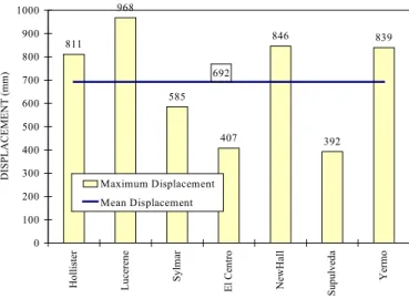
5.4 VARIATIONS IN DISPLACEMENTS 66
5.5 TIME HISTORY SEISMIC INPUT 67
5.6 RECOMMENDED RECORDS FOR TIME HISTORY ANALYSIS 67 6666 EFFECT OF ISOLATIO EFFECT OF ISOLATIOEFFECT OF ISOLATIOEFFECT OF ISOLATION ON BUILDINGSN ON BUILDINGS N ON BUILDINGSN ON BUILDINGS 70 707070
6.1 PROTOTYPE BUILDINGS 70
6.1.1 BUILDING CONFIGURATION 70
6.1.2 DESIGN OF ISOLATORS 71
6.1.3 EVALUATION PROCEDURE 77
6.1.3.1 RESPONSE SPECTRUM ANALYSIS 77
6.1.3.2 TIME HISTORY ANALYSIS 78
6.1.4.1 RESPONSE SPECTRUM ANALYSIS 79 6.1.4.2 TIME HISTORY ANALYSIS 81 6.1.5 ISOLATION SYSTEM PERFORMANCE 83 6.1.6 BUILDING INERTIA LOADS 86
6.1.6.1 RESPONSE SPECTRUM ANALYSIS 86
6.1.6.2 TIME HISTORY ANALYSIS 87
6.1.7 FLOOR ACCELERATIONS 95
6.1.7.1 RESPONSE SPECTRUM ANALYSIS 95
6.1.7.2 TIME HISTORY ANALYSIS 96
6.1.8 OPTIMUM ISOLATION SYSTEMS 100
6.2 PROBLEMS WITH THE RESPONSE SPECTRUM METHOD 102 6.2.1 UNDERESTIMATION OF OVERTURNING 102 6.2.2 REASON FOR UNDERESTIMATION 104 6.3 EXAMPLE ASSESSMENT OF ISOLATOR PROPERTIES 104 7777 ISOLATOR LOCATIONS ISOLATOR LOCATIONSISOLATOR LOCATIONSISOLATOR LOCATIONS AND TYPES AND TYPES AND TYPES AND TYPES 108108108108
7.1 SELECTION OF ISOLATION PLANE 108
7.1.1 BUILDINGS 108
7.1.2 ARCHITECTURAL FEATURES AND SERVICES 111
7.1.3 BRIDGES 112
7.1.4 OTHER STRUCTURES 112
7.2 SELECTION OF DEVICE TYPE 113
7.2.1 MIXING ISOLATOR TYPES AND SIZES 113
7.2.2 ELASTOMERIC BEARINGS 114
7.2.3 HIGH DAMPING RUBBER BEARINGS 115
7.2.4 LEAD RUBBER BEARINGS 115
7.2.5 FLAT SLIDER BEARINGS 116
7.2.6 CURVED SLIDER (FRICTION PENDULUM) BEARINGS 117
7.2.7 BALL AND ROLLER BEARINGS 118
7.2.8 SUPPLEMENTAL DAMPERS 118
7.2.9 ADVANTAGES AND DISADVANTAGES OF DEVICES 119 8888 ENGINEERIN ENGINEERINENGINEERINENGINEERING PROPERTIES OF ISOLATORSG PROPERTIES OF ISOLATORS G PROPERTIES OF ISOLATORSG PROPERTIES OF ISOLATORS 121121121121
8.1 SOURCES OF INFORMATION 121
8.2 ENGINEERING PROPERTIES OF LEAD RUBBER BEARINGS 121
8.2.1 SHEAR MODULUS 122
8.2.2 RUBBER DAMPING 122
8.2.3 CYCLIC CHANGE IN PROPERTIES 123 8.2.4 AGE CHANGE IN PROPERTIES 125
8.2.5 DESIGN COMPRESSIVE STRESS 126
8.2.6 DESIGN TENSION STRESS 127
8.2.7 MAXIMUM SHEAR STRAIN 128
8.2.8 BOND STRENGTH 129
8.2.9 VERTICAL DEFLECTIONS 130
8.2.9.2 VERTICAL DEFLECTION UNDER LATERAL LOAD 130
8.2.10 WIND DISPLACEMENT 131
8.2.11 COMPARISON OF TEST PROPERTIES WITH THEORY 131 8.3 ENGINEERING PROPERTIES OF HIGH DAMPING RUBBER ISOLATORS 133
8.3.1 SHEAR MODULUS 133
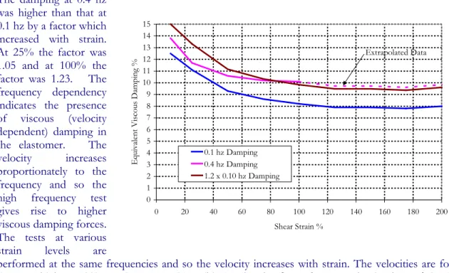
8.3.2 DAMPING 134
8.3.3 CYCLIC CHANGE IN PROPERTIES 135
8.3.4 AGE CHANGE IN PROPERTIES 135
8.3.5 DESIGN COMPRESSIVE STRESS 136
8.3.6 MAXIMUM SHEAR STRAIN 136
8.3.7 BOND STRENGTH 136
8.3.8 VERTICAL DEFLECTIONS 136 8.3.8.1 LONG TERM VERTICAL DEFLECTIONS 136
8.3.9 WIND DISPLACEMENTS 136
8.4 ENGINEERING PROPERTIES OF SLIDING TYPE ISOLATORS 137
8.4.1 DYNAMIC FRICTION COEFFICIENT 138
8.4.2 STATIC FRICTION COEFFICIENT 139
8.4.3 EFFECT OF STATIC FRICTION ON PERFORMANCE 141
8.4.4 CHECK ON RESTORING FORCE 143
8.4.5 AGE CHANGE IN PROPERTIES 143
8.4.6 CYCLIC CHANGE IN PROPERTIES 144
8.4.7 DESIGN COMPRESSIVE STRESS 144 8.4.8 ULTIMATE COMPRESSIVE STRESS 144
8.5 DESIGN LIFE OF ISOLATORS 144
8.6 FIRE RESISTANCE 144
8.7 EFFECTS OF TEMPERATURE ON PERFORMANCE 145
8.8 TEMPERATURE RANGE FOR INSTALLATION 146
9999 ISOLATION SYSTEM D ISOLATION SYSTEM DISOLATION SYSTEM DISOLATION SYSTEM DESIGNESIGNESIGNESIGN 147 147147147
9.1 DESIGN PROCEDURE 147
9.2 IMPLEMENTATION OF THE DESIGN PROCEDURE 148
9.2.1 MATERIAL DEFINITION 148
9.2.2 PROJECT DEFINITION 149
9.2.3 ISOLATOR TYPES AND LOAD DATA 150
9.2.4 ISOLATOR DIMENSIONS 152 9.2.5 ISOLATOR PERFORMANCE 153 9.2.6 PROPERTIES FOR ANALYSIS 156
9.3 DESIGN EQUATIONS FOR RUBBER AND LEAD RUBBER BEARINGS 157
9.3.1 CODES 157
9.3.2 EMPIRICAL DATA 157
9.3.3 DEFINITIONS 158
9.3.4 RANGE OF RUBBER PROPERTIES 159
9.3.5 VERTICAL STIFFNESS AND LOAD CAPACITY 160
9.3.6 VERTICAL STIFFNESS 160
9.3.7 COMPRESSIVE RATED LOAD CAPACITY 161
9.3.8 TENSILE RATED LOAD CAPACITY 163 9.3.9 BUCKING LOAD CAPACITY 163 9.3.10 LATERAL STIFFNESS AND HYSTERESIS PARAMETERS FOR BEARING 164 9.3.11 LEAD CORE CONFINEMENT 166
9.3.12 DESIGN PROCEDURE 168
9.4 SLIDING AND PENDULUM SYSTEMS 168
9.5 OTHER SYSTEMS 169
10 10 10
10 EVALUATING PERFOR EVALUATING PERFOREVALUATING PERFOREVALUATING PERFORMANCEMANCEMANCE MANCE 170170170170
10.1 STRUCTURAL ANALYSIS 170
10.2 SINGLE DEGREE-OF-FREEDOM MODEL 171
10.3 TWO DIMENSIONAL NONLINEAR MODEL 171
10.4 THREE DIMENSIONAL EQUIVALENT LINEAR MODEL 171 10.5 THREE DIMENSIONAL MODEL - ELASTIC SUPERSTRUCTURE, YIELDING ISOLATORS 172 10.6 FULLY NONLINEAR THREE DIMENSIONAL MODEL 172
10.7 DEVICE MODELING 172
10.8 ETABSANALYSIS FOR BUILDINGS 173
10.8.1 ISOLATION SYSTEM PROPERTIES 173
10.8.2 PROCEDURES FOR ANALYSIS 175
10.8.3 INPUT RESPONSE SPECTRA 176
10.8.4 DAMPING 176
10.9 CONCURRENCY EFFECTS 177
11 11 11
11 CONNECTION DESIGNCONNECTION DESIGNCONNECTION DESIGNCONNECTION DESIGN 180 180180180
11.1 ELASTOMERIC BASED ISOLATORS 180
11.1.1 DESIGN BASIS 181
11.1.2 DESIGN ACTIONS 181
11.1.3 CONNECTION BOLT DESIGN 182
11.1.4 LOAD PLATE DESIGN 183
11.2 SLIDING ISOLATORS 184
11.3 INSTALLATION EXAMPLES 184
12 12 12
12 STRUCTURAL DESIGNSTRUCTURAL DESIGNSTRUCTURAL DESIGNSTRUCTURAL DESIGN 191191191191
12.1 DESIGN CONCEPTS 191
12.2 UBC REQUIREMENTS 192
12.2.1 ELEMENTS BELOW THE ISOLATION SYSTEM 192
12.2.2 ELEMENTS ABOVE THE ISOLATION SYSTEM 193 12.3 MCE LEVEL OF EARTHQUAKE 196
12.4 NONSTRUCTURAL COMPONENTS 196
12.5 BRIDGES 197
13 13 13
13 SPECIFICATIONSSPECIFICATIONSSPECIFICATIONSSPECIFICATIONS 199199199199
13.1 GENERAL 199
14 14 14
14 BUILDING EXAMPLEBUILDING EXAMPLEBUILDING EXAMPLEBUILDING EXAMPLE 202202202202
14.1 SCOPE OF THIS EXAMPLE 202
14.2 SEISMIC INPUT 202
14.3 DESIGN OF ISOLATION SYSTEM 204
14.4 ANALYSIS MODELS 205
14.5 ANALYSIS RESULTS 206
14.5.1 SUMMARY OF RESULTS 209
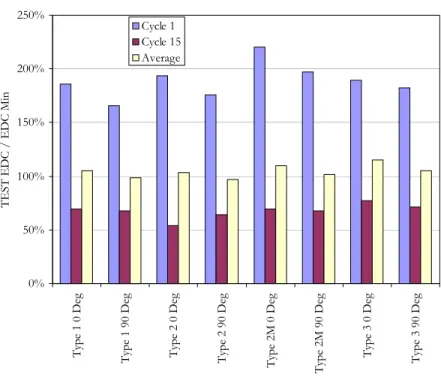
14.6 TEST CONDITIONS 210
14.7 PRODUCTION TEST RESULTS 210
14.8 SUMMARY 211
15 15 15
15 BRIDGE EXAMPLEBRIDGE EXAMPLEBRIDGE EXAMPLEBRIDGE EXAMPLE 213213213213
15.1 EXAMPLE BRIDGE 213
15.2 DESIGN OF ISOLATORS 213
15.2.1 BASE ISOLATION DESIGN 213
15.2.2 ENERGY DISSIPATION DESIGN 215
15.3 EVALUATION OF PERFORMANCE 215
15.3.1 ANALYSIS PROCEDURE 215
15.3.2 EFFECT OF ISOLATION ON DISPLACEMENTS 216
15.3.3 EFFECT OF ISOLATION ON FORCES 217
15.4 SUMMARY 218
16 16 16
16 INDUSTRIAL EQUIPMINDUSTRIAL EQUIPMINDUSTRIAL EQUIPMINDUSTRIAL EQUIPMENT EXAMPLEENT EXAMPLE ENT EXAMPLEENT EXAMPLE 219219219219
16.1 SCOPE OF THIS EXAMPLE 219
16.2 ISOLATOR DESIGN 219
16.3 SEISMIC PERFORMANCE 221
16.4 ALTERNATE ISOLATION SYSTEMS 221
16.5 SUMMARY 222
17 17 17
17 PERFORMANCE IN REPERFORMANCE IN REPERFORMANCE IN REPERFORMANCE IN REAL EARTHQUAKESAL EARTHQUAKES AL EARTHQUAKESAL EARTHQUAKES 224 224224224 18
18 18
LIST OF FIGURES
LIST OF FIGURES
LIST OF FIGURES
LIST OF FIGURES
FIGURE 1-1 BASE ISOLATION... 2
FIGURE 1-2 DESIGN FOR 1G EARTHQUAKE LOADS... 3
FIGURE 1-3 DUCTILITY... 4
FIGURE 2-1 TRANSMISSION OF GROUND MOTIONS... 9
FIGURE 2-2 STRUCTURE ACCELERATION AND DISPLACEMENT... 10
FIGURE 2-3 PERIOD SHIFT EFFECT ON ACCELERATIONS... 11
FIGURE 2-4 PERIOD SHIFT EFFECT ON DISPLACEMENT... 12
FIGURE 2-5 EFFECT OF DAMPING ON ACCELERATIONS... 16
FIGURE 2-6 EFFECT OF DAMPING ON DISPLACEMENTS... 16
FIGURE 2-7 EL CENTRO 1940: ACCELERATION SPECTRA... 18
FIGURE 2-8 EL CENTRO 1940 N-S DISPLACEMENT SPECTRA... 18
FIGURE 2-9 NORTHRIDGE SEPULVEDA: ACCELERATION SPECTRA... 19
FIGURE 2-10 NORTHRIDGE SEPULVEDA: DISPLACEMENT SPECTRA... 19
FIGURE 2-11 B FACTOR FOR 10% DAMPING: ACCELERATION... 20
FIGURE 2-12 B FACTOR FOR 10% DAMPING: DISPLACEMENT... 20
FIGURE 2-13 B FACTOR FOR 30% DAMPING: ACCELERATION... 21
FIGURE 2-14 B FACTOR FOR 30% DAMPING: DISPLACEMENT... 21
FIGURE 2-15 : : : : EQUIVALENT VISCOUS DAMPING... 22
FIGURE 2-16 NONLINEAR ACCELERATION SPECTRA... 23
FIGURE 2-17 NONLINEAR DISPLACEMENT SPECTRA... 23
FIGURE 2-18 HYSTERETIC DAMPING VERSUS DISPLACEMENT... 29
FIGURE 3-1 ISOLATING ON A SLOPE... 36
FIGURE 4-1 TYPICAL ISOLATION CONCEPT FOR BRIDGES... 50
FIGURE 4-2 EXAMPLE "KNOCK-OFF" DETAIL... 51
FIGURE 4-3 BRIDGE BEARING DESIGN PROCESS... 55
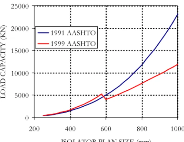
FIGURE 4-4 ELASTOMERIC BEARING LOAD CAPACITY... 56
FIGURE 5-1 SMARTS 5% DAMPED ACCLERATION SPECTRA... 61
FIGURE 5-2 SMARTS 5% DAMPED DISPLACEMENT SPECTRA... 61
FIGURE 5-3 1940 EL CENTRO EARTHQUAKE... 61
FIGURE 5-4 1952 KERN COUNTY EARTHQUAKE... 61
FIGURE 5-5 1979 EL CENTRO EARTHQUAKE : BONDS CORNER RECORD... 63
FIGURE 5-6 1985 MEXICO CITY EARTHQUAKE... 63
FIGURE 5-7 1989 LOMA PRIETA EARTHQUAKE... 63
FIGURE 5-8 1992 LANDERS EARTHQUAKE... 64
FIGURE 5-9 1994 NORTHRIDGE EARTHQUAKE... 64
FIGURE 5-10 1994 NORTHRIDGE EARTHQUAKE... 64
FIGURE 5-11 ACCELERATION RECORD WITH NEAR FAULT CHARACTERISTICS... 65
FIGURE 6-1 PROTOTYPE BUILDINGS... 70
FIGURE 6-2 SYSTEM DEFINITION... 71
FIGURE 6-3 UBC DESIGN SPECTRUM... 71
FIGURE 6-4 HDR ELASTOMER PROPERTIES... 73
FIGURE 6-5 ISOLATION SYSTEM HYSTERESIS... 76
FIGURE 6-6 EFFECTIVE STIFFNESS... 77
FIGURE 6-7 COMPOSITE RESPONSE SPECTRUM... 78
FIGURE 6-8 5% DAMPED SPECTRA OF 3 EARTHQUAKE RECORDS... 78
FIGURE 6-9 ISOLATOR RESULTS FROM RESPONSE SPECTRUM ANALYSIS COMPARED TO DESIGN... 79
FIGURE 6-10 SPECTRUM RESULTS FOR LRB1 T=1.5 SECONDS... 81
FIGURE 6-11 ISOLATOR RESULTS FROM TIME HISTORY ANALYSIS COMPARED TO DESIGN... 82
FIGURE 6-12 TIME HISTORY RESULTS FOR LRB1 T=1.5 SEC... 83
FIGURE 6-13 VARIATION BETWEEN EARTHQUAKES... 83
FIGURE 6-14 ISOLATOR PERFORMANCE : BASE SHEAR COEFFICIENTS... 85
FIGURE 6-15 ISOLATOR PERFORMANCE : ISOLATOR DISPLACEMENTS... 85
FIGURE 6-16 RESPONSE SPECTRUM INERTIA FORCES... 87
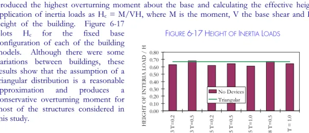
FIGURE 6-17 HEIGHT OF INERTIA LOADS... 88
FIGURE 6-18 EFFECTIVE HEIGHT OF INERTIA LOADS FOR ISOLATION SYSTEMS... 91
FIGURE 6-19 TIME HISTORY INERTIA FORCES : 3 STORY BUILDING T = 0.2 SECONDS... 92
FIGURE 6-20 TIME HISTORY INERTIA FORCES 5 STORY BUILDING T = 0.5 SECONDS... 93
FIGURE 6-21 TIME HISTORY INERTIA FORCES 8 STORY BUILDING T = 1.0 SECONDS... 94
FIGURE 6-22 RESPONSE SPECTRUM FLOOR ACCELERATIONS... 95
FIGURE 6-23 FLOOR ACCELERATIONS 3 STORY BUILDING T = 0.2 SECONDS... 97
FIGURE 6-24 FLOOR ACCELERATIONS 5 STORY BUILDING T = 0.5 SECONDS... 98
FIGURE 6-25 FLOOR ACCELERATIONS 8 STORY BUILDING T = 1.0 SECONDS... 99
FIGURE 6-26 EXAMPLE FRAME... 102
FIGURE 6-27 AXIAL LOADS IN COLUMNS... 103
FIGURE 6-28 DISPLACEMENT VERSUS BASE SHEAR... 106
FIGURE 6-29 DISPLACEMENT VERSUS FLOOR ACCELERATION... 106
FIGURE 6-30 FLOOR ACCELERATION PROFILES... 107
FIGURE 7-1 BUILDING WITH NO BASEMENT... 108
FIGURE 7-2 INSTALLATION IN BASEMENT... 109
FIGURE 7-3 FLAT JACK... 110
FIGURE 7-4 CONCEPTUAL RETROFIT INSTALLATION... 111
FIGURE 7-5 LOAD CAPACITY OF ELASTOMERIC BEARINGS... 114
FIGURE 7-6 LEAD RUBBER BEARING SECTION... 116
FIGURE 7-7 CURVED SLIDER BEARING... 117
FIGURE 7-8 VISCOUS DAMPER IN PARALLEL WITH YIELDING SYSTEM... 119
FIGURE 8-1 LEAD RUBBER BEARING HYSTERESIS... 121
FIGURE 8-2 : : : R: UBBER SHEAR MODULUS... 122
FIGURE 8-3: : : : VARIATION IN HYSTERESIS LOOP AREA... 123
FIGURE 8-4 : VARIATION IN EFFECTIVE STIFFNESS... 123
FIGURE 8-5 CYCLIC CHANGE IN LOOP AREA... 124
FIGURE 8-6 MEAN CYCLIC CHANGE IN LOOP AREA... 125
FIGURE 8-7 TENSION TEST ON ELASTOMERIC BEARING... 127
FIGURE 8-8 COMBINED COMPRESSION AND SHEAR TEST... 131
FIGURE 8-9 HIGH DAMPING RUBBER HYSTERESIS... 133
FIGURE 8-11 VISCOUS DAMPING EFFECTS IN HDR ... 134
FIGURE 8-12 CYCLIC CHANGE IN PROPERTIES FOR SCRAGGED HDR ... 135
FIGURE 8-13 SECTION THROUGH POT BEARINGS... 137
FIGURE 8-14: COEFFICIENT OF FRICTION FOR SLIDER BEARINGS... 138
FIGURE 8-15: STATIC AND STICKING FRICTION... 141
FIGURE 8-16 TIME HISTORY WITH STICKING... 142
FIGURE 8-17 HYSTERESIS WITH STICKING... 142
FIGURE 8-18 COMBINED HYSTERESIS WITH STICKING... 142
FIGURE 8-19 EFFECT OF LOW TEMPERATURES... 145
FIGURE 9-1 ISOLATOR PERFORMANCE... 147
FIGURE 9-2 : ITERATIVE PROCEDURE FOR DESIGN... 147
FIGURE 9-3 MATERIAL PROPERTIES USED FOR DESIGN... 149
FIGURE 9-4 PROJECT DEFINITION... 150
FIGURE 9-5 ISOLATOR TYPES & LOAD DATA... 151
FIGURE 9-6 ISOLATOR DIMENSIONS... 153
FIGURE 9-7 PERFORMANCE SUMMARY... 154
FIGURE 9-8 PERFORMANCE AT MCE LEVEL... 156
FIGURE 9-9 HYSTERESIS OF ISOLATORS... 156
FIGURE 9-10 ANALYSIS PROPERTIES FOR ETABS... 157
FIGURE 9-11 EFFECTIVE COMPRESSION AREA... 160
FIGURE 9-12 : : : : LEAD RUBBER BEARING HYSTERESIS... 164
FIGURE 9-13: EFFECT OF LEAD CONFINEMENT... 167
FIGURE 10-1 DISPLACEMENTS WITH CONCURRENT LOADS... 178
FIGURE 10-2 SHEARS WITH CONCURRENT LOADS... 178
FIGURE 11-1 TYPICAL INSTALLATION IN NEW BUILDING... 180
FIGURE 11-2: FORCES ON BEARING IN DEFORMED SHAPE... 181
FIGURE 11-3: EQUIVALENT COLUMN FORCES... 181
FIGURE 11-4: ASSUMED BOLT FORCE DISTRIBUTION... 182
FIGURE 11-5: SQUARE LOAD PLATE... 183
FIGURE 11-6: CIRCULAR LOAD PLATE... 183
FIGURE 11-7 EXAMPLE INSTALLATION : NEW CONSTRUCTION... 185
FIGURE 11-8 EXAMPLE INSTALLATION : EXISTING MASONRY WALL... 186
FIGURE 11-9 EXAMPLE INSTALLATION : EXISTING COLUMN... 187
FIGURE 11-10EXAMPLE INSTALLATION : EXISTING MASONRY WALL... 188
FIGURE 11-11 EXAMPLE INSTALLATION : STEEL COLUMN... 189
FIGURE 11-12 EXAMPLE INSTALLATION : STEEL ENERGY DISSIPATOR... 190
FIGURE 12-1 LIMITATION ON B ... 195
FIGURE 13-1 SPECIFICATION CONTENTS... 199
FIGURE 14-1 5% DAMPED ENVELOPE SPECTRA... 203
FIGURE 14-2 SUMMARY OF ISOLATION DESIGN... 204
FIGURE 14-3 HYSTERESIS TO MAXIMUM DISPLACEMENT... 205
FIGURE 14-4 : ETABS MODEL... 205
FIGURE 14-5 ETABS PROPERTIES... 206
FIGURE 14-7 : BASE SHEAR COEFFICIENT... 207
FIGURE 14-8 : MAXIMUM DRIFT RATIOS... 208
FIGURE 14-9: DBE EARTHQUAKE 3 INPUT... 208
FIGURE 14-10 : DBE EARTHQUAKE 3 : BEARING DISPLACEMENT... 208
FIGURE 14-11 : DBE EARTHQUAKE 3 : STORY SHEAR FORCES... 209
FIGURE 14-12 EXAMPLE PRODUCTION TEST... 212
FIGURE 15-1 : LONGITUDINAL SECTION OF BRIDGE... 214
FIGURE 15-2: TRANSVERSE SECTION OF BRIDGE... 214
FIGURE 15-3 LONGITUDINAL DISPLACEMENTS... 215
FIGURE 15-4 TRANSVERSE DISPLACEMENTS... 216
FIGURE 15-5 LONGITUDINAL DISPLACEMENTS... 216
FIGURE 15-6 TRANSVERSE DISPLACEMENTS... 217
FIGURE 15-7 LONGITUDINAL FORCES... 217
FIGURE 15-8 TRANSVERSE FORCES... 217
LIST OF TABLES
LIST OF TABLES
LIST OF TABLES
LIST OF TABLES
TABLE 1-1 ISOLATION DESIGN AND EVALUATION TOOLS... 6
TABLE 1-2ISOLATION SYSTEM SUPPLIERS... 7
TABLE 2-1 BASE SHEAR COEFFICIENT VERSUS DISPLACEMENT... 14
TABLE 2-2 UBC AND AASHTO DAMPING COEFFICIENTS... 15
TABLE 2-3 FEMA-273 DAMPING COEFFICIENTS... 15
TABLE 2-4 COMPARISON OF DAMPING FACTORS... 17
TABLE 2-5 EFFECT OF FLEXIBILITY + DAMPING... 24
TABLE 2-6 DESIGN TO CONSTANT FORCE COEFFICIENT... 26
TABLE 2-7 DESIGN TO CONSTANT DISPLACEMENT... 27
TABLE 3-1 A SUITABILITY CHECK LIST... 37
TABLE 3-2 PROCUREMENT STRATEGIES... 40
TABLE 3-3 DAMAGE RATIOS DUE TO DRIFT... 46
TABLE 3-4 DAMAGE RATIOS DUE TO FLOOR ACCELERATION... 46
TABLE 3-5 ISOLATION COSTS AS RATIO TO TOTAL BUILDING COST... 47
TABLE 3-6 SUITABLE BUILDINGS FOR ISOLATION... 49
TABLE 5-1 AVERAGE 5% DAMPED SPECTRUM VALUES... 60
TABLE 5-2 RECORDS AT SOIL SITES > 10 KM FROM SOURCES... 69
TABLE 5-3 RECORDS AT SOIL SITES NEAR SOURCES... 69
TABLE 6-1 UBC DESIGN FACTORS... 72
TABLE 6-2 ISOLATION SYSTEM VARIATIONS... 75
TABLE 6-3 ISOLATION SYSTEM PERFORMANCE (MAXIMUM OF ALL BUILDINGS, ALL EARTHQUAKES) ... 80
TABLE 6-4 OPTIMUM ISOLATION SYSTEMS... 101
TABLE 6-5 HEIGHT OF INERTIA LOADS... 103
TABLE 6-6 OPTIMUM ISOLATOR CONFIGURATION... 107
TABLE 7-1 DEVICE ADVANTAGES AND DISADVANTAGES... 120
TABLE 8-1 BENECIA-MARTINEZ ISOLATORS... 124
TABLE 8-2 COMBINED SHEAR AND TENSION TESTS... 128
TABLE 8-3: HIGH SHEAR TEST RESULTS... 129
TABLE 8-4 SKELLERUP INDUSTRIES LRB TEST RESULTS... 132
TABLE 8-5 : MINIMUM/MAXIMUM STATIC FRICTION... 140
TABLE 8-6 CALCULATION OF RESTORING FORCE... 143
TABLE 9-1 VULCANIZED NATURAL RUBBER COMPOUNDS... 159
TABLE 10-1 ANALYSIS OF ISOLATED STRUCTURES... 170
TABLE 12-1 STRUCTURAL SYSTEMS ABOVE THE ISOLATION INTERFACE... 193
TABLE 14-2 : SUMMARY OF RESULTS... 209
TABLE 14-3 PROTOTYPE TEST CONDITIONS... 210
TABLE 14-4 SUMMARY OF 3 CYCLE PRODUCTION TEST RESULTS... 211
TABLE 16-1 : ISOLATOR DIMENSIONS (MM) ... 219
TABLE 16-2 : SEISMIC PERFORMANCE (UNITS MM) ... 221
TABLE 16-3 : ALTERNATE SYSTEMS FOR BOILER... 222
TABLE 16-4 : ALTERNATE SYSTEMS FOR ECONOMIZER... 222
1111
INTRODUCTION
INTRODUCTION
INTRODUCTION
INTRODUCTION
Most structural engineers have at least a little knowledge of what base isolation is – a system of springs installed at the base of a structure to protect against earthquake damage. They know less about the when and why – when to use base isolation and why use it? When it comes to how, they either have too little knowledge or too much knowledge. Conflicting claims from promoters and manufacturers are confusing, contradictory and difficult to fully assess. Then, if a system can be selected from all the choices, there is the final set of hows – how to design the system, how to connect it to the structure, how to evaluate its performance and how to specify, test and build it. And, of course, the big how, how much does it cost?
These notes attempts to answer these questions, in sufficient detail for our practicing structural engineers, with little prior knowledge of base isolation, to evaluate whether isolation is suitable for their projects; decide what is the best system; design and detail the system; and document the process for construction.
The emphasis here is on design practice. The principles and mathematics of base isolation have been dealt with in detail in textbooks which contain rigorous treatments of the structural dynamics (see the two textbooks listed in the Bibliography, by Skinner, Robinson and McVerry [1993] and by Naiem and Kelly [1999]). These notes provide sufficient depth for our engineers to understand how the dynamics effect response but do not provide instructions as to how to solve the non-linear equations of motion governing the system response. As for much else in structural engineering, we have computer programs to do this part of the work for us.
1.1 THE CONCEPT OF BASE ISOLATION
The term base isolation uses the word isolation in its meaning of the state of being separated and base as a part that supports from beneath or serves as a foundation for an object or structure (Concise Oxford Dictionary). As suggested in the literal sense, the structure (a building, bridge or piece of equipment) is separated from its foundation. The original terminology of base isolation is more commonly replaced with seismic isolation nowadays, reflecting that in some cases the separation is somewhere above the base – for example, in a bridge the superstructure may be separated from substructure columns. In another sense, the term seismic isolation is more accurate anyway in that the structure is separated from the effects of the seism, or earthquake.
Intuitively, the concept of separating the structure from the ground to avoid earthquake damage is quite simple to grasp. After all, in an earthquake the ground moves and it is this ground movement which causes most of the damage to structures. An airplane flying over an earthquake is not affected. So, the principle is simple. Separate the structure from the ground. The ground will move but the building will not move. As in so many things, the devil is in the detail. The only way a structure can
be supported under gravity is to rest on the ground. Isolation conflicts with this fundamental structural engineering requirement. How can the structure be separated from the ground for earthquake loads but still resist gravity?
Ideal separation would be total. Perhaps an air gap, frictionless rollers, a well-oiled sliding surface, sky hooks, magnetic levitation. These all have practical restraints. An air gap would not provide vertical support; a sky-hook needs to hang from something; frictionless rollers, sliders or magnetic levitation would allow the building to move for blocks under a gust of wind.
So far, no one has solved the problems associated with ideal isolation systems and they are unlikely to be solved in the near future. In the meantime, earthquakes are causing damage to structures and their contents, even for well designed buildings. So, these notes do not deal with ideals but rather with practical isolation systems, systems that provide a compromise between attachment to the ground to resist gravity and separation from the ground to resist earthquakes.
When we define a new concept, it is often helpful to compare it with known concepts. Seismic isolation is a means of reducing the seismic demand on the structure:
Rolling with the punch is an analogy
first used by Arnold [1983?]. A boxer can stand still and take the full force of a punch but a boxer with any sense will roll back so that the power of the punch is dissipated before it reaches its target. A structure without isolation is like the upright boxer, taking the full force of the earthquake; the isolated building rolls back to reduce the impact of the earthquake.
Automobile suspension. A vehicle with no suspension system would transmit shocks from every bump and pothole in the road directly to the occupants. The suspension system has springs and dampers which modify the forces so the occupants feel very little of the motion as the wheels move over an uneven surface. As we’ll see later, this is a good analogy as springs and dampers are essential components of any practical isolation system
The party trick with the tablecloth. You’ve probably seen the party trick where the tablecloth on a fully laden table is pulled out sideways very fast. If it’s done right, everything on the table will remain in place and even unstable objects such as full glasses will not overturn. The cloth forms a sliding isolation system so that the motion of the cloth is not transmitted into the objects above.
FIGURE 1-1BASE ISOLATION
GROUND MOVES
STRUCTURE STAYS STILL
Base Isolation falls into general category of Passive Energy Dissipation, which also includes In-Structure Damping. In-structure damping adds damping devices within the structure to dissipate energy but does not permit base movement. This technique for reducing earthquake demand is covered in separate HCG Design Guidelines. The other category of earthquake demand reduction is termed Active Control, where isolation and/or energy dissipation devices are powered to provide optimum performance. This category is the topic of active research but there are no widely available practical systems and our company has no plans to implement this strategy in the short term.
1.2 THE PURPOSE OF BASE ISOLATION
A high proportion of the world is subjected to earthquakes and society expects that structural engineers will design our buildings so that they can survive the effects of these earthquakes. As for all the load cases we encounter in the design process, such as gravity and wind, we work to meet a single basic equation:
CAPACITY > DEMAND
We know that earthquakes happen and are uncontrollable. So, in that sense, we have to accept the demand and make sure that the capacity exceeds it. The earthquake causes inertia forces proportional to the product of the building mass and the earthquake ground accelerations. As the ground accelerations increases, the
strength of the building, the capacity, must be increased to avoid structural damage.
It is not practical to continue to increase the strength of the building indefinitely. In high seismic zones the accelerations causing forces in the building may exceed one or even two times the acceleration due to gravity, g. It is easy to visualize the strength needed for this level of load – strength to resist 1g means than the building could resist gravity applied sideways, which means that the building could be tipped on its side and held horizontal without damage.
Designing for this level of strength is not easy, nor cheap. So most codes allow engineers to use ductility to achieve the capacity. Ductility is a concept of allowing the structural elements to deform beyond their elastic limit in a controlled manner. Beyond this limit, the structural elements soften and the displacements increase with only a small increase in force.
The elastic limit is the load point up to which the effects of loads are non-permanent; that is, when the load is removed the material returns to its initial condition. Once this elastic limit is exceeded changes occur. These changes are permanent and non-reversible when the load is removed. These
changes may be dramatic – when concrete exceeds its elastic limit in tension a crack forms – or subtle, such as when the flange of a steel girder yields.
For most structural materials, ductility equals structural damage, in that the effect of both is the same in terms of the definition of damage as that which impairs the usefulness of the object. Ductility will generally cause visible damage. The capacity of a structure to continue to resist loads will be impaired.
A design philosophy focused on capacity leads to a choice of two evils: 1. Continue to increase the elastic
strength. This is expensive and for buildings leads to higher floor accelerations. Mitigation of structural damage by further
strengthening may cause more damage to the contents than would occur in a building with less strength.
2. Limit the elastic strength and detail for ductility. This approach accepts damage to structural components, which may not be repairable.
Base isolation takes the opposite approach, it attempts to reduce the demand rather than increase the capacity. We cannot control the earthquake itself but we can modify the demand it makes on the structure by preventing the motions being transmitted from the foundation into the structure above. So, the primary reason to use isolation is to mitigate earthquake effects. Naturally, there is a cost associated with isolation and so it only makes sense to use it when the benefits exceed this cost. And, of course, the cost benefit ratio must be more attractive than that available from alternative measures of providing earthquake resistance.
1.3 A BRIEF HISTORY OF BASE ISOLATION
Although the first patents for base isolation were in the 1800’s, and examples of base isolation were claimed during the early 1900’s (e.g. Tokyo Imperial Hotel) it was the 1970’s before base isolation moved into the mainstream of structural engineering. Isolation was used on bridges from the early 1970’s and buildings from the late 1970’s. Bridges are a more natural candidate for isolation than buildings because they are often built with bearings separating the superstructure from the substructure.
The first bridge applications added energy dissipation to the flexibility already there. The lead rubber bearing (LRB) was invented in the 1970’s and this allowed the flexibility and damping to be included
FIGURE 1-3 DUCTILITY
For
c
e
Deformation Elastic
Limit
in a single unit. About the same time the first applications using rubber bearings for isolation were constructed. However, these had the drawback of little inherent damping and were not rigid enough to resist service loads such as wind.
In the early 1980’s developments in rubber technology lead to new rubber compounds which were termed “high damping rubber” (HDR). These compounds produced bearings that had a high stiffness at low shear strains but a reduced stiffness at higher strain levels. On unloading, these bearings formed a hysteresis loop that had a significant amount of damping. The first building and bridge applications in the U.S. in the early 1980’s used either LRBs or HDR bearings.
Some early projects used sliding bearings in parallel with LRBs or HDR bearings, typically to support light components such as stairs. Sliding bearings were not used alone as the isolation system because, although they have high levels of damping, they do not have a restoring force. A structure on sliding bearings would likely end up in a different location after an earthquake and continue to dislocate under aftershocks.
The development of the friction pendulum system (FPS) shaped the sliding bearing into a spherical surface, overcoming this major disadvantage of sliding bearings. As the bearing moved laterally it was lifted vertically. This provided a restoring force.
Although many other systems have been promulgated, based on rollers, cables etc., the market for base isolation now is mainly distributed among variations of LRBs, HDR bearings, flat sliding bearings and FPS.
In terms of supply, the LRB is now out of patent and so there are competing suppliers in most parts of the world. Although specific HDR compounds may be protected, a number of manufacturers have proprietary compounds that provide the same general level of performance. The FPS system is patented but there are licensees in most parts of the world.
1.4 THE HOLMES ISOLATION TOOLBOX
The main differences between design of an isolated structure compared to non-isolated structures are that the isolation devices need to be designed and the level of analysis required is usually higher. We have developed tools to assist in each of these areas.
Isolation System Design
The isolator design is governed by a relatively small number of equations and does not require extensive numerical computation and so can be performed using spreadsheet tools. We have template spreadsheets developed for the codes we will normally encounter (UBC, NZS4203 and AASHTO) as listed in Table 1-1. These spreadsheets are described further later but are able to design most commonly used isolators. The performance is estimated based on a single mass approximation, effectively assuming a rigid building above the isolators.
The other spreadsheet listed in Table 1-1, Bridge, incorporates the AASHTO bearing design procedures but has the analysis built in. This is because bridge models are generally simpler than building models. The Bridge spreadsheet can perform a single mode analysis, including the effects of
flexible piers and eccentricity under transverse loads, and also shells to a non-linear time history analysis using a modified version of the Drain-2D computer program. Dynamic analysis results are imported to the spreadsheet for comparison with single mode results.
Isolation System Evaluation
Evaluation of base isolated structures usually requires a dynamic analysis, either response spectrum or time history. Often we do both. For buildings, the ETABS program can be used for both types of analysis provided a linear elastic structure is appropriate. The DUCTILEIN and DUCTILEOUT pre- and post-processors can be used with isolated buildings. If the structure is not suited to ETABS but non-linearity is restricted to the isolation system then SAP2000 has similar capabilities to ETABS and is more suited to general-purpose finite element modeling.
If non-linearity of the structural system needs to be modeled then use the ANSR-L program. This is general purpose and is suited to both buildings and other types of structure. Use the MODELA and PROCESSA pre- and post-processors with this program. This program is also suited to multiple analyses, for example, to examine a large number of options for the isolation system parameters. 3D-BASIS is a special purpose program for analysis of base isolation buildings. It uses the structural model developed for ETABS as a super-element. We do not use this program very often now that ETABS has non-linear isolation elements but it may be more efficient for multiple batched analyses, similar to ANSR-L.
TABLE 1-1 ISOLATION DESIGN AND EVALUATION TOOLS
Name Type Purpose
UBCTemplate NZS4203Template AASHTO Template BRIDGE
.xls .xls .xls .xls
Design isolators to UBC provisions.
As above but modified for NZS4203 seismic loads. Design isolators to 1999 AASHTO provisions. as above with Analysis Modules
ETABS SAP2000 3D-BASIS ANSR-L
.exe .exe .exe .exe
Analysis of linear buildings with non-linear isolators Analysis of linear structures with non-linear isolators. Analysis of linear buildings with non-linear isolators Analysis of non-linear structures with nonlinear isolators. DUCTILEIN
DUCTILEOUT MODELA PROCESSA
.xls .xls .xls .xls
Prepare models for ETABS Process results from ETABS Prepare models for ANSR-L Process results from ANSR-L
ACCEL .xls 5% Damped spectrum of earthquake records
Far fault has 36 records distant from faults Near fault has 10 near fault records Contains procedure for UBC scaling
1.5 ISOLATION SYSTEM SUPPLIERS
There are continual changes in the list of isolation system suppliers as new entrants commence supply and existing suppliers extend their product range. The system suppliers listed in Table 1-2 are companies which we have used in our isolation projects, who have supplied to major projects for other engineers or who have qualified in the HITEC program. HITEC is a program operated in the U.S. by the Highway Technology Innovation Center for qualification of isolation and energy dissipation systems for bridges.
Given the changes in the industry, this list may be outdated quickly. You can find out current information on these suppliers from the web and may also identify suppliers not listed below.
The project specifications should ensure that potential suppliers have the quality of product and resources to supply in a timely fashion. This may require a pre-qualification process.
There are a large number of manufacturers of elastomeric bearings worldwide as these bearings are widely used for bridge pads and bearings for non-isolation purposes. These manufacturers may offer to supply isolation systems such as lead-rubber and high damping rubber bearings. However, standard bridge bearings are designed to operate at relatively low strain levels of about 25%. Isolation bearings in high seismic zones may be required to operate at strain levels ten times this level, up to 250%. The manufacturing processes required to achieve this level of performance are much more stringent than for the lower strain levels. In particular, the bonding techniques are critical and the facilities must be of clean-room standard to ensure no contamination of components during assembly. Manufacturers not included in Table 1-2 should be required to provide evidence that their product can achieve the performance levels required of seismic isolators.
TABLE 1-2ISOLATION SYSTEM SUPPLIERS
Company Product
Bridgestone (Japan) BTR Andre (UK)
Scougal Rubber Corporation (US)
High damping rubber
Robinson Seismic (NZ) Lead rubber
Earthquake Protection Systems, Inc (US) Friction pendulum system Dynamic Isolation Systems, Inc (US)
Skellerup Industries (NZ) Seismic Energy Products (US)
Lead rubber, high damping rubber Hercules Engineering (Australia) Pot (sliding) bearings
R J Watson, Inc (US)
FIP-Energy Absorption Systems (US) Sliding Bearings Taylor Devices, Inc. (US)
1.6 ISOLATION SYSTEM DURABILITY
Many isolation systems use materials which are not traditionally used in structural engineering, such as natural or synthetic rubber or polytetrafluoroethylene (PTFE, which is used for sliding bearings, usually known as Teflon ©, which is DuPont’s trade name for PTFE). An often expressed concern of structural engineers considering the use of isolation is that these components may not have a design life as long as other structural components, usually considered to be 50 years or more.
Natural rubber has been used as an engineering material since the 1840’s and some of these early components remained in service for nearly a century in spite of their manufacturers lacking any knowledge of protecting elastomers against degradation. Natural rubber bearings used for applications such as gun mountings from the 1940’s remain in service today.
Elastomeric (layered rubber and steel) bearings have been in use for about 40 years for bridges and have proved satisfactory over this period. Shear testing on 37 year old bridge bearings showed an average increase in stiffness of only 7% and also showed that oxidation was restricted to distances from 10 mm to 20 mm from the surface. Since these early bearings were manufactured technology for providing resistance to oxygen and ozone degradation has improved and so it is expected that modern isolation bearings would easily exceed a 50 year design life.
Some early bridge bearings were cold bonded (glued, rather than vulcanized) and these bearings had premature failures, damping the reputation of isolation bearings. The manufacture of all elastomeric bearings isolation bearings is by vulcanization; the steel plates are sand blasted and de-greased, stacked in a mold in parallel with the rubber layers and the assembly is then cured under heat and pressure. Curing may take 24 hours or more for very large isolators.
Some bridge bearings are manufactured from synthetic rubbers, usually neoprene. There are reports that neoprene will stiffen with age to a far greater extent than natural rubber and this material does not appear to have been used for isolation bearings for this reason. If a manufacturer suggests a synthetic elastomer, be sure to request extensive data on the effects of age on the properties.
PTFE was invented in 1938 and has been used extensively for all types of applications since the 1940’s. It is virtually inert to all chemicals and is about the best material known to man for corrosion resistance, which is why there is difficulty in etching and bonding it. Given these properties, it should last almost indefinitely. In base isolation applications the PTFE slides on a stainless steel surface under high pressure and velocity and there is some flaking of the PTFE and these flakes are deposited on the stainless steel surface. Eventually the bearing will wear out but indications are that this will occur after travel of between 10 km and 20 km. For buildings this is not a concern as sliding occurs only during earthquake and the total travel is measured in meters rather than kilometers. For bridges the PTFE is often lubricated with silicone grease contained by dimples in the PTFE.
2222
PRINCIPLES OF BASE ISOLATION
PRINCIPLES OF BASE ISOLATION
PRINCIPLES OF BASE ISOLATION
PRINCIPLES OF BASE ISOLATION
2.1 FLEXIBILITY – THE PERIOD SHIFT EFFECT
2.1.1 THE PRINCIPLE
The fundamental principle of base isolation is to modify the response of the building so that the ground can move below the building without transmitting these motions into the building. In an ideal system this separation would be total. In the real world, there needs to be some contact between the structure and the ground.
A building that is perfectly rigid will have a zero period. When the ground moves the acceleration induced in the structure will be equal to the ground acceleration and there will be zero relative displacement between the structure and the ground. The structure and ground move the same amount.
A building that is perfectly flexible will have an infinite period. For this type of structure, when the ground beneath the structure moves there will be zero acceleration induced in the structure and the relative displacement between the structure and ground will be equal to the ground displacement. The structure will not move, the ground will.
FIGURE 2-1 TRANSMISSION OF GROUND MOTIONS
FLEXIBLE STRUCTURE RIGID STRUCTURE
Zero Acceleration Ground Acceleration
Ground Displacement No
All real structures are neither perfectly rigid nor perfectly flexible and so the response to ground motions is between these two extremes, as shown in Figure 2-2. For periods between zero and infinity, the maximum accelerations and displacements relative to the ground are a function of the earthquake, as shown conceptually in Figure 2-2.
For most earthquakes there be a range of periods at which the acceleration in the structure will be amplified beyond the maximum ground acceleration. The relative displacements will generally not exceed the peak ground displacement, that is the infinite period displacement, but there are some exceptions to this, particularly for soft soil sites and site which are located close to the fault generating the earthquake.
FIGURE 2-2STRUCTURE ACCELERATION AND DISPLACEMENT
Ac
c
e
le
ra
ti
o
n
Di
s
p
lacem
en
t
A
ccel
er
at
io
n
Di
s
p
lacem
en
t
RIGID FLEXIBLE
2.1.2 EARTHQUAKE CHARACTERISTICS
The reduction in acceleration response when the period is lengthened is a result of the characteristics of earthquake motions. Although we generally approach structural design using earthquake accelerations or displacements, it is the velocity that gives the best illustration of the effects of isolation. The energy input from an earthquake is proportional to the velocity squared.
Implementation of base isolation in codes is based on the assumption that over the mid-frequency range, for periods of about 0.5 seconds to 4 seconds, the energy input is a constant, that is, the velocity is constant. Design codes such as the UBC and NZS4203 assume this. For a constant velocity, the displacement is proportional to the period, T, and the acceleration is inversely proportional to T. If the period is doubled, the displacement will double but the acceleration will be halved.
2.1.3 CODE EARTHQUAKE LOADS
The period shift effect can be calculated directly from code specified earthquake loads. Code specifications generally provide a base shear coefficient, C, as a function of period. This coefficient is a representation of the spectral acceleration such that C times the acceleration due to gravity, g, provides an acceleration in units of time/length2.
Figures 2-3 and 2-4 show the period shift effect on accelerations and displacements. The curves on these figures are for a high seismic zone and are based on the coefficients defined by FEMA-273 and UBC. They show that the period shift effect is most effectively if short period structures (T < 1 second) are isolated to 2 seconds or more.
FIGURE 2-3PERIOD SHIFT EFFECT ON ACCELERATIONS
0.000 0.200 0.400 0.600 0.800 1.000 1.200 1.400 1.600 1.800 2.000
0.000 0.500 1.000 1.500 2.000 2.500 3.000 3.500 4.000
PERIOD (Seconds)
ACCE
LE
R
A
T
ION
(g
)
FEMA-273 BSE-2 FEMA 273-BSE-1 UBC
FIGURE 2-4PERIOD SHIFT EFFECT ON DISPLACEMENT
0.0 5.0 10.0 15.0 20.0 25.0 30.0 35.0 40.0 45.0 50.0
0.000 0.500 1.000 1.500 2.000 2.500 3.000 3.500 4.000
PERIOD (Seconds)
D
ISPL
A
C
E
ME
NT (
inches
)
FEMA-273 BSE-2 FEMA 273-BSE-1 UBC
Period Shift Effect
The displacements in Figure 2-4 are calculated from the code shear coefficient. For any code that specifies a design coefficient, C, the acceleration represented by this coefficient can be converted to a pseudo-spectral displacement, Sd, using the relationship:
2
ω
gC d
S =
Where ω is the circular frequency, in radians per cycle. This is related to the period as
T 2π ω=
From which the displacement, ∆, can be calculated as
2
4
π
2
gCT
d
S
∆
=
=
For most codes, beyond a minimum period up to which the base shear coefficient is a constant, the velocity is assumed constant and the base shear coefficient is inversely proportional to T, that is,
T C
C= v
Where Cv is a constant related to factors such as soil type, seismicity, near fault effects etc. In this
zone, the product of displacement and shear coefficient is a constant:
=
2 2v
4
π
g
C
∆
C
In this equation, Cv is code specific. The constant related to units of length, g/4π2, has a numerical
value of 248.5 for mm units and 9.788 for inch units.
The fact that this product is constant provides a clear illustration of the trade off between base shear coefficient, C, and the displacement, ∆. If you want to reduce the base shear coefficient by a factor of 2 then the displacements will double. If you want to reduce the coefficient by 4, the displacements will increase by a factor of 4.
As an example, consider a UBC design in Zone 4 with a near fault factors of Na = 1.2 and Nv = 1.6,
Soil Profile SB. The seismic coefficients are Ca = 0.48 and Cv = 0.64. The period beyond which the
velocity is assumed constant is calculated as 0.533
2.5C C T
a v
s = =
For periods beyond 0.533 seconds, the product ∆C = 248.5 x 0.642 = 101.8 in mm units (4.01 in inch
units).
Table 2-1 shows the relationship between base shear coefficient and displacement for this example. At the transition period, 0.53 seconds, the coefficient is 1.2. If you want to reduce this by a factor of 4, to 0.30, the displacement will be 339 mm (13.4 inches). At this displacement the period can be calculated as Cv / C = 0.64/0.30 = 2.13 seconds.
Most codes specify coefficients based on 5% damping and the values in Table 2-1 are based on this. As discussed later, the displacements associated with adding damping to the system can reduce the period shift effect.
Although the example above is based on the UBC, a similar function can be derived for any code that specifies the coefficient as an inverse function of period:
• Calculate the coefficient, C at any period, T, beyond the transition period. • Calculate the displacement, ∆, at this period as 248.5CT2 mm (9.788CT2 inches).
• The product of C∆ can now be used as a constant to calculate the displacement at any other base shear coefficient C1 as ∆1 = C∆/C1.
TABLE 2-1BASE SHEAR COEFFICIENT VERSUS DISPLACEMENT
Base Shear
Coefficient Maximum Displacement Period,T
C mm inch (seconds)
1.20 85 3.3 0.53
1.10 93 3.6 0.58
1.00 102 4.0 0.64
0.90 113 4.5 0.71
0.80 127 5.0 0.80
0.70 145 5.7 0.91
0.60 170 6.7 1.07
0.50 204 8.0 1.28
0.40 254 10.0 1.60
0.35 291 11.5 1.83
0.30 339 13.4 2.13
0.25 407 16.0 2.56
0.20 509 20.0 3.20
0.15 679 26.7 4.27
2.2 ENERGY DISSIPATION – ADDING DAMPING
Damping is the characteristic of a structural system that opposes motion and tends to return the system to rest when it is disturbed. Damping arises from a multitude of sources. For isolation systems, damping is generally categorized as viscous (velocity dependent) or hysteretic (displacement dependent). For equivalent linear analysis, hysteretic damping is converted to equivalent viscous damping.
Whereas the period shift effect usually decreases acceleration but increases displacements, damping almost always decreases both accelerations and displacement. A warning here, increased damping reduces accelerations in respect to the base shear, which is dominated by first mode response. However, high damping may increase accelerations in higher modes of the structure. For multi-story buildings, the statement that “the more damping the better” may not hold true.
Response spectra provided in codes are almost invariably for 5% damping. There are several procedures available for modifying spectra for damping ratios other than 5%.
The Eurocode EC8 provides a formula for the acceleration at damping ξ relative to the acceleration at 5% damping as:
ξ
ξ =∆ +
∆
2 7
) 5 , ( ) ,
(T t
Where ξ is expressed as a percent of critical damping. UBC and AASHTO provide tabulated B coefficients, as listed in Table 2-2. FEMA-273 provides a different factor for short and long periods, as listed in Table 2-4. Generally the factor Bl would apply for all isolated structures. This has the
same values as the UBC and AASHTO values in Table 2-2.
TABLE 2-2UBC AND AASHTO DAMPING COEFFICIENTS
Equivalent Viscous Damping
<2% 5% 10% 20% 30% 40% >50%
B 0.8 1.0 1.2 1.5 1.7 1.9 2.0
In Table 2-3 the reciprocal of the EC8 value is listed alongside the equivalent factors from FEMA-273. EC8 provides for a greater reduction due to damping than the other codes and seem to relate to the short period values, Bs, from FEMA-273.
TABLE 2-3FEMA-273 DAMPING COEFFICIENTS
Effective Damping ββββ
% of Critical
Bs Periods ≤≤≤≤ To
Bl Periods > To
EC8
< 2 5 10 20 30 40 > 50
0.8 1.0 1.3 1.8 2.3 2.7 3.0
0.8 1.0 1.2 1.5 1.7 1.9 2.0
0.75 1.00 1.31 1.77 2.14 2.45 2.73
Figures 2-5 and 2-6 plot the effect of damping on isolated accelerations and displacements respectively using UBC / AASHTO values of B. Both quantities are inversely proportional to the damping coefficient, B, and so the damping reduces both by the same relative amount.
FIGURE 2-5EFFECT OF DAMPING ON ACCELERATIONS
0.000 0.200 0.400 0.600 0.800 1.000 1.200 1.400 1.600 1.800 2.000
0.000 0.500 1.000 1.500 2.000 2.500 3.000 3.500 4.000
PERIOD (Seconds)
ACCE
LE
R
A
T
ION
(g
)
5 % Damping 10% Damping 20% Damping Increased
Damping Effect
FIGURE 2-6EFFECT OF DAMPING ON DISPLACEMENTS
0.0 5.0 10.0 15.0 20.0 25.0 30.0 35.0 40.0 45.0 50.0
0.000 0.500 1.000 1.500 2.000 2.500 3.000 3.500 4.000
PERIOD (Seconds)
ACCE
LE
R
A
T
ION
(g
)
5 % Damping 10% Damping
20% Damping Increased
Damping Effect
2.2.1 HOW ACCURATE IS THE B FACTOR?
The accuracy of the B factor can be assessed by generating response spectra for various damping ratios and comparing these with the spectra reduced by the B factor. Two records were chosen for this comparison:
1. The N-S component of the 1940 El Centro earthquake. This was one of the first strong motion records of high amplitude recorded and has been the basis for many studies. Figure 2-7 shows the acceleration spectra for this record and Figure 2-8 the equivalent displacement spectra, each for damping ratios from 5% to 40% of critical.
2. The Los Angeles, Sepulveda V.A. Hospital, 360 degree component of the record from the 1994 Northridge earthquake. This record was only 8 km (5 miles) from the epicenter of the 1994 earthquake and so exhibits near fault effects. Figures 2.9 and 2.10 show the respective acceleration and displacement spectra for the same damping values as for the El Centro record. The near fault Sepulveda record produces a much greater response than the more distance El Centro record, a peak spectral acceleration of 2.8g compared to 0.9g and peak spectral displacement of 550 mm (22”) versus 275 mm (11”) for 5% damping. The impact of this on isolation design is discussed later.
The actual B factors from these records can be calculated at each period by dividing the spectral acceleration or displacement at a particular damping by the equivalent value at the 5% damping. Figures 2-11 to 2-14 plot these B factors for 10% and 30% damping and compare them with the B values from the UBC and EC.
The first point to note is that the use of a constant B factor is very much an approximation. The actual reduction in response due to viscous damping in a function of both the period and the earthquake record. As the B factor is a single value function, Table 2-4 compares it with the mean values calculated from the spectra for periods from 0.5 to 4 seconds, the period range for isolation systems.
TABLE 2-4COMPARISON OF DAMPING FACTORS
10 % Damping 30% Damping
Acceleration Displacement Acceleration Displacement
Average From Spectra El Centro
Sepulveda 0.840.83 0.810.80 0.650.70 0.490.47
UBC 0.83 0.83 0.59 0.59
The UBC B factor for 10% damping is a good representation of the mean for the two examples considered here, for both acceleration and displacement response. For 30% damping the higher damping tends to reduce displacements by a greater proportion than accelerations. For this level, the UBC factor is non-conservative for accelerations and conservative for displacements compared to the mean value. The EC factor tends to overestimate the effects of damping across the board. Given the uncertainties in the earthquake motions, the UBC B factor appears to be a reasonable approximation but you need to be aware that is just than, an approximation. To get a more accurate response to a particular earthquake you will need to generate damped spectra or run a time history analysis.
FIGURE 2-7EL CENTRO 1940: ACCELERATION SPECTRA
0.00 0.10 0.20 0.30 0.40 0.50 0.60 0.70 0.80 0.90 1.00
0.00 0.50 1.00 1.50 2.00 2.50 3.00 3.50 4.00 PERIOD (Seconds)
A
CCEL
E
R
A
TION
(g
)
5.0% 10.0% 20.0% 30.0% 40.0%
FIGURE 2-8EL CENTRO 1940 N-S DISPLACEMENT SPECTRA
0.0 50.0 100.0 150.0 200.0 250.0 300.0
0.00 0.50 1.00 1.50 2.00 2.50 3.00 3.50 4.00 PERIOD (Seconds)
DI
SP
L
A
C
E
M
E
NT
(g
)
5.0% 10.0% 20.0% 30.0% 40.0%
FIGURE 2-9NORTHRIDGE SEPULVEDA: ACCELERATION SPECTRA
0.00 0.50 1.00 1.50 2.00 2.50 3.00
0.00 0.50 1.00 1.50 2.00 2.50 3.00 3.50 4.00
PERIOD (Seconds)
A
CCEL
E
RA
T
IO
N
(g
)
5.0% 10.0% 20.0% 30.0% 40.0%
FIGURE 2-10NORTHRIDGE SEPULVEDA: DISPLACEMENT SPECTRA
0.0 100.0 200.0 300.0 400.0 500.0 600.0
0.00 0.50 1.00 1.50 2.00 2.50 3.00 3.50 4.00
PERIOD (Seconds)
DI
SPLACE
ME
NT (
g)
5.0% 10.0% 20.0% 30.0% 40.0%
FIGURE 2-11B FACTOR FOR 10% DAMPING: ACCELERATION
0.60 0.65 0.70 0.75 0.80 0.85 0.90 0.95 1.00
0.000 0.500 1.000 1.500 2.000 2.500 3.000 3.500 4.000
PERIOD (Seconds)
A
CCE
L
E
RA
T
ION /
A
CCE
L
E
RA
T
ION A
T
5
%
El Centro Sepulveda UBC 10% EC8 10%
FIGURE 2-12B FACTOR FOR 10% DAMPING: DISPLACEMENT
0.60 0.65 0.70 0.75 0.80 0.85 0.90 0.95 1.00
0.000 0.500 1.000 1.500 2.000 2.500 3.000 3.500 4.000
PERIOD (Seconds)
DI
SPLACE
ME
NT / DI
SPLACE
ME
NT AT 5%
El Centro Sepulveda UBC 10% EC8 10%
FIGURE 2-13B FACTOR FOR 30% DAMPING: ACCELERATION
0.30 0.40 0.50 0.60 0.70 0.80 0.90 1.00
0.000 0.500 1.000 1.500 2.000 2.500 3.000 3.500 4.000
PERIOD (Seconds)
ACCE
LE
RAT
IO
N
/ ACCE
LE
RAT
IO
N
AT
5%
El Centro Sepulveda UBC 30% EC8 30%
FIGURE 2-14BFACTOR FOR 30% DAMPING: DISPLACEMENT
0.30 0.40 0.50 0.60 0.70 0.80 0.90 1.00
0.000 0.500 1.000 1.500 2.000 2.500 3.000 3.500 4.000
PERIOD (Seconds)
DI
SPLACE
ME
NT / DI
SPLACE
ME
NT AT 5%
El Centro Sepulveda UBC 30% EC8 30%
2.2.2 TYPES OF DAMPING
Base isolation codes represent damping arising from all sources as equivalent viscous damping, damping which is a function of velocity. Most types of isolators provide damping which is classified as hysteretic, damping which is a function of displacement.
The conversion of hysteretic damping to equivalent viscous damping, β, is discussed later but for a given displacement, ∆, is based on calculating:
∆
=
22
1
eff h
K
A
π
β
Where Ah is the area of the hysteresis loop and Keff is the effective stiffness of the isolator at
displacement ∆, as shown in Figure 2.15.
FIGURE 2-15: : : E: QUIVALENT VISCOUS DAMPING
The accuracy of using the damping factor, B, is not well documented but it appears to produce results generally consistent with a nonlinear analysis.
Figures 2-16 and 2-17 compare the results from an equivalent elastic analysis with the results from a series of nonlinear analyses using 7 earthquakes each frequency scaled to match the design spectrum. For all practical isolation periods (T > 1 second) the approximate procedure produces a result which
falls between the maximum and minimum values from the nonlinear analyses. As the effective period increases beyond 2 seconds the approximate procedure tends to give results close to the mean of the nonlinear analyses.
The example given is for a single isolation system yield level and design spectral shape. However, unpublished research appears to show that the equivalent elastic approach does produce results that fall within nonlinear analysis bounds for most practical conditions. The B factor approach has the advantage that the curves shown on Figures 2-16 and 2-17 can be produced using a spreadsheet rather than a nonlinear analysis program.
FIGURE 2-16NONLINEAR ACCELERATION SPECTRA
Bi-Linear System Fy = 0.05 W
0.00 0.20 0.40 0.60 0.80 1.00 1.20 1.40
0.00 0.50 1.00 1.50 2.00 2.50 3.00
Effective Period (Seconds)
Accelera
tion (g)
Calculated Using B Factor
Nonlinear Analysis Maximum of 7 Earthquakes Nonlinear Analysis Minimum of 7 Earthquakes
FIGURE 2-17NONLINEAR DISPLACEMENT SPECTRA
Bi-Linear System Fy = 0.05 W
0.00 50.00 100.00 150.00 200.00 250.00 300.00
0.00 0.50 1.00 1.50 2.00 2.50 3.00
Effective Period (Seconds)
Displa
cement (mm)
Calculated Using B Factor
Nonlinear Analysis Maximum of 7 Earthquakes Nonlinear Analysis Minimum of 7 Earthquakes
2.3 FLEXIBILITY + DAMPING
Of the two main components of the isolation system, flexibility and damping, the former generally has the greatest effect on response modification, especially if the building mounted on the isolation system has a relatively short period, less than about 0.7 seconds.
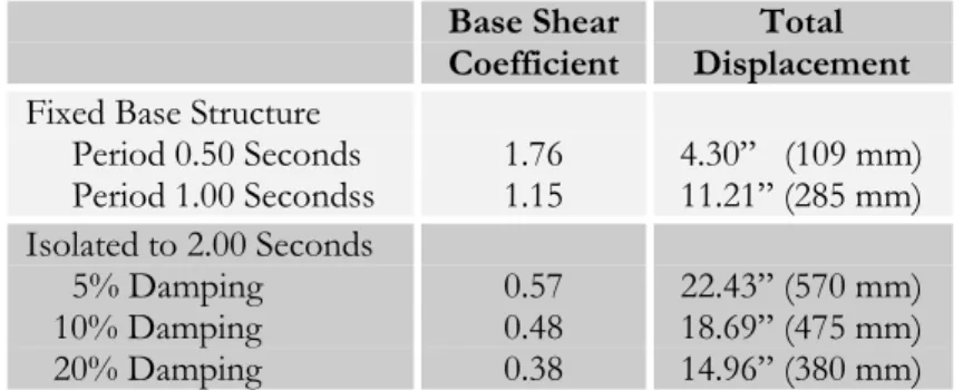
Table 2-5 lists the base shear coefficients and displacements for a structure in a high seismic zone with near fault effects. In terms of displacements;
• If the structure is stiff, with a period of 0.50 seconds, a 5% damped isolation system with a 2-second period will reduce the coefficient from 1.76 to 0.57, a reduction by a factor of 3. If the damping of the isolation system is increased from 5% to 20% the coefficient reduces to 0.38, two-thirds the 5% damped value.
• If the structure is more flexible, with a period of 1.00 seconds, the 5% damped isolation system with a 2-second period will reduce the coefficient from 1.15 to 0.57, a reduction by a factor of 2. The effect of the damping increase from 5% to 20% remains the same, the coefficient reduces to 0.38, two-thirds the 5% damped value.
The reduction in acceleration response due to the flexibility of the isolation system depends on the stiffness of the building but the reduction due to damping is independent of the building stiffness.
TABLE 2-5EFFECT OF FLEXIBILITY + DAMPING
Base Shear
Coefficient DisplacementTotal
Fixed Base Structure Period 0.50 Seconds
Period 1.00 Secondss 1.761.15 4.30” (109 mm)11.21” (285 mm) Isolated to 2.00 Seconds
5% Damping 10% Damping 20% Damping
0.57 0.48 0.38
22.43” (570 mm) 18.69” (475 mm) 14.96” (380 mm)
In terms of displacements, the flexibility effect of increasing the period to 2.0 seconds increases the displacements but the damping reduces this displacement. For the fixed base structure the displacement occurs at the centroid of the building, approximately two-thirds the building height. For the isolated building most displacement occurs across the isolation plane, with a lesser amount occurring within the structure.