MICHAEL SHULMAN
Abstract. We observe that the Reedy model structure on a diagram category can be constructed by iterating an operation of “bigluing” model structures along a pair of functors and a natural transformation. This yields a new explanation of the definition of Reedy categories: they are almost exactly those small categories for which the category of diagrams and its model structure can be constructed by iterated bigluing. It also gives a consistent way to produce generalizations of Reedy categories, including the generalized Reedy categories of Cisinski and Berger–Moerdijk and the enriched Reedy categories of Angeltveit, but also new versions such as a combined notion of “enriched generalized Reedy category”.
Contents
1. Introduction 1
2. Weak factorization systems and model categories 5
3. Bigluing of model categories 8
4. Inverse categories, with an introduction to collages 12
5. Functoriality of bigluing 18
6. Iterated bigluing 20
7. Reedy categories 26
8. Generalized Reedy categories 36
9. Enriched Reedy categories 47
10. Enriched generalized Reedy categories 54
Appendix A. Functorially-Reedy categories 59
Appendix B. Remarks on the formalization 62
References 64
1. Introduction
1.1. Overview. In the preprint [Ree], Reedy described an inductive procedure for defining simplicial objects and maps between them, and used it to construct a fairly explicit model structure on the category of simplicial objects in any model category. Kan then generalized this model structure to diagrams indexed by any
Date: June 29, 2015.
This material is based on research sponsored by The United States Air Force Research Laboratory under agreement number FA9550-15-1-0053. The U.S. Government is authorized to reproduce and distribute reprints for Governmental purposes notwithstanding any copyright notation thereon. The views and conclusions contained herein are those of the author and should not be interpreted as necessarily representing the official policies or endorsements, either expressed or implied, of the United States Air Force Research Laboratory, the U.S. Government, or Carnegie Mellon University.
Reedy category, a notion he defined by abstracting some properties of the domain category∆op for simplicial objects. The notion of Reedy category has since become standard in the model-categorical literature, appearing among other places in the books [Hov99, Ch. 5], [Hir03, Ch. 15], [DHKS04,§22]1, [Lur09,§A.2.9], and [Rie14, Ch. 14].
However, there is no obvious reason why Kan’s definition is the only or the
best context in which to formulate Reedy’s construction abstractly. And indeed, several people have generalized the definition of Reedy category, maintaining the important property that Reedy diagrams in a model category inherit a fairly explicit model structure. For instance, Cisinski [Cis06, Def. 8.1.1] and Berger– Moerdijk [BM11] have modified the definition to allow a Reedy category to contain nontrivial automorphisms, while Angeltveit [Ang08] has given a version for enriched categories. However, none of these definitions appear inevitable either. Perhaps the most satisfying account of Reedy categories to date is that of Riehl and Verity [RV14], who show that Kan’s definition implies a decomposition of the hom-functor as a cell complex, which in turn induces analogous decompositions of all diagrams. But the definition of Reedy category itself is still taken as given.
In this paper we analyze Reedy categories and Reedy model structures from the other direction: instead of “what is a Reedy category?” we ask “what is a Reedy model structure?” and work backwards to the definition of a Reedy category. The classical result is that ifC is a Reedy category andMa model category, then the diagram categoryMC has a model structure in which a map A→B is
• . . . a weak equivalence iffAx→Bxis a weak equivalence inMfor allx∈ C.
• . . . a cofibration iff the induced mapAxtLxALxB→Bxis a cofibration inM for allx∈ C.
• . . . a fibration iff the induced mapAx→Bx×MxBMxAis a fibration inMfor allx∈ C.
HereLx andMx are thelatching object andmatching object functors, which are defined in terms of the Reedy structure of C. However, at the moment all we care about is that if xhas degreen(part of the structure of a Reedy category is an ordinal-valued degree function on its objects), then Lx and Mx are functors
MCn → M, where C
n is the full subcategory of C on the objects of degree less thann. In the prototypical example of ∆op, whereMC is the category of simplicial
objects inM,LnAis the “object of degeneraten-simplices” whereasMnA is the “object of simplicial (n−1)-spheres (potential boundaries forn-simplices)”.
The fundamental observation which makes the Reedy model structure tick is that if we have a diagram A∈ MCn, then to extend it to a diagram defined at
xas well, it is necessary and sufficient to give an object Ax and a factorization
LxA→Ax→MxAof the canonical mapLxA→MxA(and similarly for morphisms of diagrams). For ∆op, this means that if we have a partially defined simplicial object with objects ofk-simplices for all k < n, then to extend it withn-simplices we have to give an object An, a mapLnA→An including the degeneracies, and a mapAn→MnAassigning the boundary of every simplex, such that the composite
LnA→An→MnAassigns the correct boundary to degenerate simplices.
Categorically speaking, this observation can be reformulated as follows. Given a natural transformationα:F →Gbetween parallel functorsF, G:M → N, let us define thebigluing categoryG`(α) to be the category of quadruples (M, N, φ, γ) such
thatM ∈ M,N ∈ N, andφ:F M →Nandγ:N →GM are a factorization ofαM throughN. The above observation is then thatMCx ' G`(α), whereα:L
x→Mx
is the canonical map between functorsMCn→ MandC
xis the full subcategory of
ConCn∪ {x}. Moreover, it is an easy exercise to reformulate the usual construction of the Reedy model structure as a theorem that ifMandN are model categories andF andGare left and right Quillen respectively, thenG`(α) inherits a model structure.
Therefore, our answer to the question “what is a Reedy model structure?” is that it is one obtained by repeatedly (perhaps transfinitely) bigluing along a certain kind of transformation between functorsMC → M(whereCis a category playing the
role ofCn previously). This motivates us to ask, givenC, how can we find functors
F, G :MC → M and a map α: F →Gsuch that G`(α) is of the form MC0 for some new categoryC0?
Of course, we expect C0 to be obtained fromC by adding one new object “x”.
Thus, it stands to reason thatF,G, andαwill have to specify, among other things, the morphismsfrom xtoobjects in C, and the morphismsto xfrom objects ofC. These two collections of morphisms form diagrams W :C →Set and U :Cop→Set, respectively; and given such U and W we do have canonical functors F and G, namely the U-weighted colimit and the W-weighted limit. Moreover, a natural transformation from theU-weighted colimit to theW-weighted limit can naturally be specified by giving a mapW ×U →C( –,– ) in SetCop×C. InC0, this map will supply the composition of morphisms throughx.
It remains only to specify the hom-setC0(x, x) (and the relevant composition
maps), and for this there is a “universal choice”: we takeC0(x, x) = (W⊗
CU)t{idx}. That is, we throw in composites of morphisms x→y →x, freely subject to the associative law, and also an identity morphism. This C0 has a universal property
(it is a “collage” in the bicategory of profunctors) which ensures that the resulting biglued category is indeed equivalent toMC0
.
A category with degrees assigned to its objects can be obtained by iterating this construction if and only if any nonidentity morphism between objects of the same degree factors uniquely-up-to-zigzags through an object of strictly lesser degree (i.e. the category of such factorizations is connected). What remains is to ensure that the resulting latching and matching objects are left and right Quillen. It turns out that this is equivalent to requiring that morphisms between objects of different
degrees also have connected or empty categories of factorizations through objects of strictly lesser degree. For a precise statement, seeDefinition 7.9; we will call these almost-Reedy categories.
This doesn’t look much like the usual definition of Reedy category, but it turns out to be very close to it. If C is almost-Reedy, let −→C (resp. ←−C) be the class of morphismsf :x→y such that deg(x)≤deg(y) (resp. deg(y)≤deg(x)) and that do not factor through any object of strictly lesser degree than xandy. We will show that just as in a Reedy category, every morphism factors uniquely into a
←−
C-morphism followed by a−→C-morphism.
The only thing missing from the usual definition of a Reedy category, therefore, is that←−C and−→C be subcategories, i.e. closed under composition. And indeed, this can fail to be true; seeExample 7.19. However, this is all that can go wrong: C is a Reedy category if and only if it is an almost-Reedy category such that←−C and−→C
to be given as data in the definition of a Reedy category; they are recoverable from the degree function. This was also noticed by [RV14].)
It is unclear whether the extra generality of almost-Reedy categories is useful: it is more difficult to verify in practice and seems unlikely to have natural applications. The point is rather that the notion of Reedy category (very slightly generalized) arises inevitably from the process of iterated bigluing.
Moreover, as often happens when we reformulate a definition more conceptually, it becomes easier to generalize. Iterated bigluing can also be applied to more general types of input data, unifying various sorts of generalized Reedy-like categories in a common framework. For instance, bigluing withMG rather thanMitself, whereG
is a groupoid, yields essentially the notion ofgeneralized Reedy category from [BM11]. Bigluing withMD for an arbitrary categoryDyields a “more generalized” notion
of Reedy category. Bigluing enriched categories instead yields a notion ofenriched Reedy category that generalizes the definition of [Ang08]. Finally, combining these two generalizations we obtain a new notion ofenriched generalized Reedy category. Other potential generalizations also suggest themselves; the idea of “Reedy-ness” as presented here applies naturally in any “category theory” where we have profunctors and collages. For instance, one could considerinternal Reedy categories in a well-behaved model category, orenriched indexed Reedy categories in the sense of [Shu13].
1.2. Outline. Insection 2we make some simple observations about model categories and weak factorization systems which may not be exactly in the literature. Then insection 3 we introduce the bigluing construction that forms the foundation of the paper. But rather than jumping right into its application to Reedy categories, to smooth the exposition insection 4 we first describe the special case ofinverse categories, which correspond to the special case of bigluing calledgluing. This allows us to introduce the central idea ofcollages in a less complicated setting.
Insection 5we return to the general theory of bigluing, proving some functoriality results that are necessary for the application to Reedy categories. Then insection 6
we study general diagram categories that are obtained by iterated bigluing, and their domains, which we callbistratified categories. Reedy categories are a special sort of bistratified category; they are almost exactly those bistratified categories with discrete strata whose diagram categories inherit model structures from the bigluing construction. Insection 7we explain this: we introduce the intermediate notion ofalmost-Reedy category, which areprecisely the above class of bistratified categories, and show that Reedy categories are the almost-Reedy categories for which−→C and←−C are closed under composition. The proof of this makes essential use of a factorization lemma which was also central to [RV14]. We show furthermore that Reedy categories are also exactly the almost-Reedy categories such that latching and matching objects can be computed as colimits and limits over−→C and←C−only, respectively; this gives an additional argument for their naturalness.
The last few sections are concerned with generalizations. Insection 8 we relax the requirement of discrete strata, obtaining a notion ofc-Reedy category which generalizes the “generalized Reedy categories” of [BM11]. In [BM11] the strata are required to be groupoids; we can even do without that hypothesis. In section 9
we generalize instead to enriched category theory, obtaining a notion ofReedy V -category which generalizes the ReedyV-categories of [Ang08]. Finally, insection 10
which permits non-discrete strata. As an example, we show that the construction in [Ang08] of a Reedy V-category associated to a non-symmetric operad can be generalized to symmetric operads.
1.3. Prerequisites. Technically, this paper does not depend on any prior knowledge of Reedy categories, or even their definition. However, space does not permit the inclusion of appropriate motivation and examples for this paper to serve as a good
introduction to Reedy categories. Thus I recommend the reader have some previous acquaintance with them; this can be obtained from any of the books cited in the first paragraph of this introduction. I will also assume familiarity with basic notions of model category theory, which can be obtained from the same sources.
1.4. A Formalization. This paper is slightly unusual, for a paper in category theory, in that one of its main results (Theorem 7.16: almost-Reedy categories are almost Reedy categories) depends on a sequence of technical lemmas, and as far as I know there is no particular reason toexpect it to be true. That Reedy categories are almost-Reedy is essentially necessitated by the fact that Kan’s definition suffices to construct Reedy model structures, but I have no intuitive argument for why adding closure under composition is enough for the converse; it just happens to work out that way. Thus, it is natural to worry that a small mistake in one of the technical lemmas might bring the whole theorem crashing down.
To allay such concerns (which I shared myself), I have formally verified this theorem using the computer proof assistant Coq. Verifying all the results of this paper would require a substantial library of basic category theory, but fortunately the proof ofTheorem 7.16(including the technical lemmas) is largely elementary, requiring little more than the definition of a category. (In fact, the formalization is a proof of the more general Theorem 8.26, assuming as given the elementary characterization of almost-c-Reedy categories fromTheorem 8.13.) The Coq code is available online from my website; inAppendix Bbelow I include some remarks on how it relates to the proofs as given in the paper proper.
1.5. Acknowledgments. I would like to thank Emily Riehl for several useful discussions about [RV14] and feedback on a draft of this paper; David White for drawing my attention to the existing terminology “couniversal weak equivalence” (Definition 3.9); Karol Szumi lo for the proof of Lemma 7.7; Michal Przybylek for
the example in footnote 4; Charles Rezk for Example A.2; and Justin Noel for a conversation about enriched generalized Reedy categories. Some of the results herein were obtained independently (and a little earlier) by Richard Garner. I would also like to thank Arthur, for sleeping peacefully while I wrote this paper.
2. Weak factorization systems and model categories Recall the following definitions.
Definition 2.1. A weak factorization system, or wfs, on a category Mis a pair (L,R) of classes of maps such that
(i) L is the class of maps having the left lifting property with respect toR, (ii) Ris the class of maps having the right lifting property with respect toL, and (iii) Every morphism inMfactors as a map inLfollowed by a map inR. Definition 2.2. Amodel structureonMis a triple (C,F,W) of classes of maps such that
• (C ∩ W,F) and (C,F ∩ W) are wfs, and
• W satisfies the 2-out-of-3 property.
This is equivalent to Quillen’s original definition of (closed) model category; it can be found in [MP12, 14.2.1] or [Rie14, 11.3.1]. If there is only one wfs of interest on a category, we denote it by (L,R); context makes it clear which category we are referring to. We say that a morphismf :X →Y in Lis anL-map, and thatX is anL-objectif∅ →X is anL-map. Dually, we speak ofR-maps andR-objects.
We will also occasionally need the following weaker notion.
Definition 2.3. Apre-wfsis a pair (L,R) satisfyingDefinition 2.1(i)and(ii), but not necessarily(iii).
Our main reason for considering pre-wfs is the following examples.
Lemma 2.4. If Mis a complete and cocomplete category with a pre-wfs andC is any small category, thenMC has two pre-wfs defined as follows:
• In theprojective pre-wfs, the R-maps are the natural transformations that are objectwise inR, withLbeing the maps having the left lifting property with respect to these.
• In theinjective pre-wfs, theL-maps are the natural transformations that are objectwise inL, withRbeing the maps having the right lifting property with respect to these.
Proof. We prove the projective case; the injective one is dual. With the definitions as given, it suffices to show that any map having the right lifting property with respect to the projectiveL-maps is objectwise inR.
Note that for any c∈ C, the functor “evaluate atc” evc :MC → M has a left
adjoint defined byM 7→ C(c,– )·M. Thus, iff :M →M0 is anL-map inM, then the induced mapC(c,– )·f :C(c,– )·M → C(c,– )·M0 has the left lifting property with respect to all mapsX →Y inMC such thatX
c →Yc is inR. In particular,
C(c,– )·f is a projectiveL-map.
But conversely,X→Y has the right lifting property with respect to all maps of the formC(c,– )·f, forf anL-map inM, if and only if Xc→Yc is inR. Thus, if
X →Y has the right lifting property with respect to all projectiveL-maps, it must
be objectwise inR.
Even if the given pre-wfs on M is a wfs, this is not necessarily the case for the projective and injective pre-wfs. This holds for the projective case if the wfs on M is cofibrantly generated, and for the injective case if M is furthermore a
locally presentable category (in which case one says that a cofibrantly generated wfs is combinatorial). In either of these cases, model structures also lift to diagram categories.
IfV,M, andN are equipped with pre-wfs andN has pushouts, we say a functor
inV andMrespectively, the induced dotted map from the pushout
S(V, M) //
S(V0, M)
$
$
S(V, M0) //
,
,
S(V, M0)tS(V,M)S(V0, M)
*
*
S(V0, M0)
is an L-map. We say that S : Vop× M → N is a right wfs-bimorphism if
Sop:V × Mop→ Nop is a left wfs-bimorphism. We will need the well-known fact that these conditions for any of the three functors in a two-variable adjunction imply the corresponding conditions for the other two; see e.g. [Rie14, Lemma 11.1.10]. Note in particular that this makes no use of factorizations, so it is true whether or not the pre-wfs in question are wfs.
The “most basic” wfs is (injections, surjections) on Set. This is “universally enriching” for all pre-wfs, in the following sense.
Theorem 2.5. IfMis complete and cocomplete and equipped with a pre-wfs, then (i) The copower functor Set× M → Mis a left wfs-bimorphism,
(ii) The power functor Setop× M → M is a right wfs-bimorphism, and (iii) The hom-functorMop× M →Setis a right wfs-bimorphism.
Proof. It suffices to prove one of(i)–(iii). The easiest is (iii), which claims that if
A→B is anL-map andC→D anR-map, then the induced function
M(B, C)→ M(A, C)×M(A,D)M(B, D)
is a surjection. But this is just the lifting property of a pre-wfs. We will need to be able to take limits of diagrams of categories equipped with wfs or pre-wfs (hence also model categories). We could do this by using either a pseudo sort of limit or a strict sort of morphism; for simplicity we choose the latter. Definition 2.6. A pre-wfs isclovenif we have chosen a particular lift in every commutative square from an L-map to an R-map. A wfs is cloven if we have additionally chosen a particular (L,R)-factorization of every morphism (which need not be functorial). Astrict functor between cloven wfs or pre-wfs is one which preservesboth classes of maps, and also the chosen lifts (and factorizations, in the wfs case) on the nose.
Let PreWfscl and Wfscl denote the category of categories with cloven pre-wfs and wfs, respectively, with strict functors between them.
Strict functors do not occur often, but the basic construction insection 3will produce them. The value of noticing this lies in the following fact.
Theorem 2.7. The forgetful functors PreWfscl → Cat and Wfscl → Cat create limits.
Proof. Define a map in limcMc to be inLorRif it becomes so in eachMc. Lifts and factorizations can be defined in eachMc, fitting together because the functors are strict. Similarly,LandRdetermine each other because they do in eachMc.
We can also take limits of functors between diagrams of cloven wfs with strict maps. Precisely, consider the following categories:
• WfsMorcl and PreWfsMorcl, whose objects are triples (M,N, F) where M
andN have cloven wfs and pre-wfs, respectively, andF :M → N preserves
L-maps (but is not strict). Its morphisms are commutative squares in which the functorsM → M0 andN → N0 are strict.
• WfsBiMorcl and PreWfsBiMorcl, whose objects are quadruples (V,M,N, S) whereV, M, andN have cloven wfs or pre-wfs,N has chosen pushouts, and
S :V × M → N is a left wfs-bimorphism. Their morphisms consist of strict functorsV → V0,M → M0, andN → N0 making the obvious square commute,
and such thatN → N0 preserves the chosen pushouts on the nose.
We have forgetful functors
WfsMorcl→Func WfsBiMorcl→BiFunc PreWfsMorcl→Func PreWfsBiMorcl→BiFunc
where Func is the category whose objects are functors and whose morphisms are commutative squares of functors, while BiFunc is the similar category whose objects are bifunctorsS:V × M → N.
Theorem 2.8. The above forgetful functors create limits.
We will primarily be interested in ordinal-indexed limits. If β is an ordinal, regarded as a category in the usual way, by a continuous β-tower we mean a continuous functor M : βop → Cat. Thus, if δ < β is a limit ordinal, we have
Mδ = limδ0<δMδ0.
The dual notion is acocontinuousβ-cotower. IfC:β →Cat is such a cotower andMis a fixed category, the universal property of colimits says that
(2.9) Mcolimδ<βCδ ∼= lim
δ<βM
Cδ.
3. Bigluing of model categories
LetMandN be categories,F, G:M → N functors, andα:F →Ga natural transformation.
Definition 3.1. Thebigluing category ofα, denotedG`(α), is defined as follows.
• An object of G`(α) consists of an objectM ∈ M, an object N ∈ N, and a factorization ofαM :F M →GM throughN, i.e. morphismsφ:F M →N and
γ:N →GM whose composite isαM.
• A morphism ofG`(α) consists of morphismsµ:M →M0 andν:N →N0 such that the following two squares commute.
F M φ //
F µ
N γ //
ν
GM
Gµ
F M0
φ0
/
/N0
γ0
/
/GM0
The gluing constructionis the special case whenF is constant at an initial object. In this case, αis uniquely determined, so we speak of gluing along the functor G and write G`(G) instead of G`(∅ → G). The objects of the resulting category consist ofM ∈ MandN∈ N together with a mapN→GM. Dually, if
Gis constant at a terminal object, we may speak ofcogluing alongF; this explains the terminology “bigluing”.
Note thatG`(α)op=G`(αop), whereαop:Gop→Fopis the induced transforma-tion between functorsMop→ Nop. There are forgetful functorsG`(α)→ Mand
G`(α)→ N.
Lemma 3.2. The forgetful functor G`(α) → M has a left adjoint with identity counit. If G has a left adjoint and N has binary coproducts, then the forgetful functorG`(α)→ N also has a left adjoint.
Proof. The first left adjoint takesM to (M, F M,id, αM).
LetK be the left adjoint of G; we now construct a left adjoint toG`(α)→ N. GivenB ∈ N, consider the object
e
KB= (KB, F KBtB, i1,[αKB, η])
of G`(α), where i1 is the coproduct injectionF KB → F KBtB, and [αKB, η] :
F KBtB →GKB has components αKB:F KB →GKB and the unitη :B →
GKB of the adjunctionKaG. A map fromKBe to (M, N, φ, γ) consists of a map
µ:KB→M andν:F KBtB→N such that the following two squares commute.
F KB i1 //
F µ
F KBtB [αKB,η] //
ν=[ν1,ν2]
GKB
Gµ
F M
φ //N γ //GM
The first square just ensures that the first component ν1 of ν is the composite
F KB → F M → N. Given this, the second square consists of naturality for α
(which is automatically true) together with the assertion that the adjunctB→GM
ofµunder the adjunctionKaGis the compositeB ν2
−→N −→γ GM. Thus, a map e
KB → (M, N, φ, γ) is uniquely determined by a map ν2 : B → N; so Ke is left
adjoint toG`(α)→ N.
Dually, we have:
Lemma 3.3. The forgetful functorG`(α)→ M has a right adjoint with identity unit. IfF has a right adjoint andN has binary products, then the forgetful functor
G`(α)→ N also has a right adjoint.
We now observe:
Lemma 3.4. If M and N are cocomplete and F is cocontinuous, then G`(α) is cocomplete. Dually, ifMand N are complete and Gis continuous, thenG`(α)is complete.
In either case, ifM andN have chosen limits or colimits, we can choose those inG`(α)to be preserved strictly by both forgetful functors.
Thus, it at least makes sense to ask whetherG`(α) inherits a model structure fromMandN. We expect to need some further conditions to make this true.
Suppose first thatMandN are equipped with wfs. In the following theorem we see the fundamental Reedy-style constructions.
Theorem 3.5. IfM and N each have a wfs and N has pushouts and pullbacks, thenG`(α)inherits a wfs defined as follows.
• TheL-maps are those whereM →M0 and the induced mapF M0tF MN →N0
are both inL.
• TheR-maps are those whereM →M0and the induced mapN→GM×GM0N0
are both inR.
If the wfs onM andN are cloven, then the wfs on G`(α)is canonically cloven and the forgetful functorG`(α)→ Mis strict.
Proof. Since both classes of maps are closed under retracts, it suffices to show the factorization and lifting properties. The construction should look familiar to any reader who has seen Reedy model structures before. We factor a morphism (µ, ν) : (M, N, φ, γ)→(M0, N0, φ0, γ0) by first factoringµas M −→L M00 R−→M0 in
M, then performing the dotted factorization below inN:
F M //
N
/
/GM
F M00 //
F M00tF MN //N00 //GM00×GM0N0
/
/GM00
F M0 //N0 //GM0
For lifting, we suppose given commutative squares
(3.6)
M1 //
M3
M2 //M4
N1 //
N3
N2 //N4 commuting with theφ’s andγ’s and such that the maps
M1→M2 and F M2tF M1N1→N2
are inL and the maps
M3→M4 and N3→GM3×GM4N4
are inR. We lift in the first square in (3.6) to obtain a mapM2→M3, then lift in the following square:
F M2tF M1N1 //
N3
N2 //GM3×GM4N4
whose top and bottom maps are induced by the given ones and the lift M2→M3. The final claim is clear from the above explicit constructions.
This is also true for pre-wfs if our functors have adjoints.
Theorem 3.7. IfMandN each have a pre-wfs, N has finite limits and colimits, and F has a right adjoint and Ghas a left adjoint, thenG`(α) inherits a pre-wfs defined as in Theorem 3.5.
Proof. It remains to show that the classesL andRin G`(α) determine each other by lifting properties. (In the case of wfs, this follows from the factorization property and closure under retracts.)
Suppose that a map (M, N, φ, γ)→(M0, N0, φ0, γ0) inG`(α) has the right lifting
property with respect toL. Since the left adjoint of the forgetful functorG`(α)→ M
preservesL-maps by inspection, the underlying map M →M0 must be inR. Now letKbe the left adjoint ofGandKe the resulting left adjoint toG`(α)→ N as inLemma 3.2. Letf :A→B be anL-map inN, and consider the object
b
Kf = (KB, F KBtA, i1,[αKB, ηf])
ofG`(α). A similar analysis to the proof ofLemma 3.2reveals that a map fromKfb to (M, N, φ, γ) consists of a commutative square
(3.8)
A //
f
N
γ
B //GM.
We have an induced mapKfb →KBe , precomposition with which induces a commu-tative square (3.8) from knowing its diagonal. It follows that to give a commutative square as on the left inG`(α):
b
Kf //
(M, N, φ, γ)
e
KB //(M0, N0, φ0, γ0)
A //
N
B //N0×GM0GM
is equivalent to giving a commutative square on the right inN, and diagonal liftings likewise correspond.
Finally, this map Kfb →KBe is in L, since idKB :KB →KB is an L-map in
MandF KBtA→F KBtB is anL-map in N (being the coproduct of the two
L-maps idF KB and f :A →B). Thus, if (M, N, φ, γ)→ (M0, N0, φ0, γ0) has the right lifting property with respect toL, then it must have the right lifting property with respect toKfb →KBe , and henceN →N0×GM0GM must be an R-map in
N, as desired.
In particular, ifMandN are model categories, then both of their constituent wfs lift toG`(α). To fit together these wfs into a model structure onG`(α), however, we need an additional hypothesis, for which purpose we recall the following definition from [BB13].
Definition 3.9. A morphismf in a model category is acouniversal weak equiv-alenceif every pushout off is a weak equivalence. Dually,f is auniversal weak equivalenceif every pullback of it is a weak equivalence.
Every acyclic cofibration is a couniversal weak equivalence. More generally, if there happens to be some other model structure on the same category with the same or smaller class of weak equivalences, then any acyclic cofibration in that other model structure will also be a couniversal weak equivalence. In addition, we have the following observation:
Lemma 3.10. Let Mbe a model category andC any small category, and suppose MC has any model structure in which the weak equivalences are objectwise. Then any objectwise acyclic cofibration inMC is a couniversal weak equivalence in this model structure, and similarly any objectwise acyclic fibration is a universal weak equivalence.
Proof. This follows immediately from the fact that limits, colimits, and weak equivalences inMC are objectwise.
Note thatLemma 3.10does not require the existence of a projective or injective model structure onMC.
Theorem 3.11. SupposeMandN are model categories and we haveF, G:M → N andα:F →Gsuch that
• Fis cocontinuous and takes acyclic cofibrations to couniversal weak equivalences. • Gis continuous and takes acyclic fibrations to universal weak equivalences. Then G`(α)is a model category, and the forgetful functors to Mand N preserve cofibrations, fibrations, and weak equivalences.
Proof. ByTheorem 3.5,G`(α) inherits two wfs which we call (cofibration, acyclic fibration) and (acyclic cofibration, fibration). (For the moment, we treat “acyclic cofibration” and “acyclic fibration” as atomic names for classes of morphisms in
G`(α).) We define a map inG`(α) to be a weak equivalence just when bothM →M0
andN →N0 are.
Now if a cofibration in G`(α) is also a weak equivalence, then its underlying mapM →M0 inMis an acyclic cofibration. HenceF M →F M0 is a couniversal weak equivalence, thus its pushoutN →F M0tF MN is a weak equivalence. Since
N →N0 is a weak equivalence, by the 2-out-of-3 property, F M0tF MN →N0 is also a weak equivalence, and hence an acyclic cofibration. Thus, our original map was an acyclic cofibration.
The same argument with the 2-out-of-3 property applied in the other direction shows that every acyclic cofibration is a weak equivalence. Thus, the acyclic cofibrations inG`(α) are precisely the cofibrations that are also weak equivalences, and dually for the acyclic fibrations. Since the weak equivalences obviously satisfy the 2-out-of-3 property, we have a model structure. Note that the hypotheses are satisfied ifF is left Quillen andGis right Quillen. The more general hypothesis will be useful in section 8.
Remark 3.12. Richard Garner has noted that the bigluing construction can be seen as an instance of the Grothendieck construction for wfs described in [Roi94,
Sta14,HP14]. Namely, whenN has pullbacks and pushouts, the forgetful functor
G`(α)→ Mis a Grothendieck bifibration (i.e. both a fibration and an opfibration), whose fiber overM ∈ Mis the category of factorizations ofαM. IfMandN have wfs, then the wfs of N also induces a wfs on these fibers, and so the Grothendieck construction yields the biglued wfs on the total categoryG`(α).
4. Inverse categories, with an introduction to collages
As a warm-up before diving into Reedy categories, we start withinverse categories. These turn out to correspond toiterated gluing in the same way that Reedy categories
will correspond to iterated bigluing (and their duals, direct categories, correspond to iterated cogluing).
As we will do later for Reedy categories, we will not assume the notion of inverse categorya priori. Instead, in this section our goal will be to construct the diagram categories MC, for some yet-to-be-determined class of categories C, by iterated gluing. Specifically, we will repeatedly glue some previously constructed category
MC withM along a functor G : MC → M. ByTheorem 3.11, if we want the
construction to preserve model structures, it is reasonable to take Gto be right Quillen. A natural class of functorsMC → M, which we may hope will at least
sometimes be right Quillen, is provided byweighted limits.
Recall that if X : C → M andW : C →Set, the W-weighted limit of X is defined to be the functor cotensor product
{W, X}C= eq
Y
c
X(c)W(c)⇒Y
c,c0
X(c)C(c0,c)×W(c0)
.
IfMis complete, this defines a functor{W,–}C :MC → M, which has a left adjoint
that sendsY ∈ Mto the copower defined by (Y ·W)(c) =Y ·W(c). In particular,
{W,–}C is continuous, so gluing along it will at least preserve completeness and
cocompleteness.
We would now like to define aninverse category to be a categoryC such that for any complete categoryM, the categoryMC can be obtained from Mby repeated
gluing along weighted limit functors. However, in order for that to be sensible, we need to know that if we glue along a weighted limit functor{W,–}C :MC → M,
the resulting category is (at least sometimes) again a diagram category MC0 for
some other categoryC0. Fortunately, as we will now show, this isalways the case.
Recall that for categoriesCandD, aprofunctorfromCtoD, denotedH :C −7−→ D, is a functor H :Dop× C → Set. Profunctors are the morphisms of a bicategory
Prof, where composition is the functor tensor product: the composite ofH :C −7−→ D
andK:D −7−→ E is defined by
(KH)(e, c) = coeq
a
d,d0
K(e, d)× D(d, d0)×H(d0, c)⇒a d
K(e, d)×H(d, c)
.
Definition 4.1. Thecollageof a profunctorH:C −7−→ D, which we will write [H], is the category whose objects are the disjoint union of those ofC andD, and whose hom-sets are
[H](c, c0) =C(c, c0) [H](d, c) =H(d, c) [H](d, d0) =D(d, d0) [H](c, d) =∅
with composition and identities induced from those of CandDand the functoriality ofH.
In particular, we may consider a weightW :C →Set to be a profunctor fromC
to the terminal category1. Its collage is then a category [W] containingC as a full subcategory, with one additional object? added, and with additional morphisms [W](?, c) =W(c).
Of central importance for us is that the collage of any profunctor has a universal property in the bicategory of profunctors: it is arepresentable lax colimit. To explain
this, recall that any functor P : C → D induces a representable profunctor
P•:C −7−→ D, defined by
P•(d, c) =D(d, P(c)).
This defines the action on morphisms of an identity-on-objects pseudofunctor ( – )•:
Cat → Prof. Moreover, this pseudofunctor is locally fully faithful, i.e. a natural transformationP→Qis uniquely determined by its imageP•→Q•. Finally, every
representable profunctorP• has a right adjoint profunctor P• defined by
P•(c, d) =D(P(c), d).
Definition 4.2. Arepresentable lax cocone with vertexE under a profunctor
H : C −7−→ D consists of functors P : D → E and Q : C → E and a natural transformationP•H →Q•. A morphism of such cocones (with the same vertex)
consists of transformations P → P0 and Q → Q0 such that an evident square
commutes.
By the adjointnessP• aP•, a transformation P•H →Q• can equivalently be
regarded as a transformationH →P•Q•. Moreover, the “co-Yoneda lemma” implies
that (P•Q•)(d, c) =∼E(P d, Qc). So a representable lax cocone under H : C −7−→ D
consists of P : D → E and Q : C → E together with “an interpretation of the elements ofH as morphisms from the image ofP to the image of Q.” This makes the following fact fairly clear.
Theorem 4.3. Any profunctorH :C −7−→ Dadmits a representable lax cocone with vertex [H], where P and Qare the inclusions and the transformation H(d, c)→
[H](P d, Qc)is the identity. Moreover, this is theuniversalrepresentable lax cocone, in the sense that the category of representable lax cocones underH with vertex E is naturally isomorphic to the category of functors [H]→ E.
In fact, [H] is also a lax colimit in the bicategoryProf: the universal representable lax cocone is also the universal non-representable lax cocone. For more on this universal property of collages, see [Str81,Woo85,GS13]. Our purpose in recalling it is to prove the following theorem.
Theorem 4.4. For any categoryC and weightW :C →Set, if we glue along the
W-weighted limit functor{W,–}C :MC → M, we have G`({W,–}C)' M[W].
Proof. In view ofTheorem 4.3, it will suffice to show thatG`({W,–}C) is equivalent
to the category of representable lax cocones underW with vertexM. By definition, an object ofG`({W,–}C) consists ofQ∈ MC andP∈ Mand a mapP → {W, Q}C.
But this is equivalent to a mapW → M(P, Q) in SetC, which we can regard as a map
W → {P•, Q•}1 inProf(C,1), if we identify the object P with the corresponding
functor1→ M. Finally, by adjunction this is equivalent to a mapP•⊗1W →Q•,
as required. (Note that our mapP → {W, Q}C is also equivalent by adjunction to a
mapP·W →QinMC, but (P·W)
• is not isomorphic toP•⊗1W, because the
Yoneda embedding does not preserve colimits.)
Therefore, the categories obtained fromMby repeated gluing along weighted limit functors are all diagram categories. So we may define theinverse categories to be the diagram shapes obtained in this way, e.g. we may define aninverse category of height0 to be the empty category, and aninverse category of heightn+ 1 to be one of the form [W], whereW :C →Set andCis an inverse category of heightn.
However, in this way we will obtain only inverse categories with finitely many objects, with a unique object being added at each positive integer height. These are sufficient for some purposes, but often we need to generalize the iteration by increasing either the “width” or the “height” (or both).
Increasing thewidth means adding more objects at each stage. This is easy to do by gluing along a functorMC → MI, whereI is a discrete set, instead of a functor
MC → M. Such a functor is just anI-indexed family of functorsMC → M, each of
which we may take to be a weighted limit {Wi,–}C for some weightsWi:C →Set. We can regard these weights together as forming a profunctor W :C −7−→I. In general, for any categoriesCandDand any profunctorW :C −7−→ D, ifMis complete then we have a functorMC → MD denoted {W,–}C, defined by
{W, X}C(d) ={W(d,– ), X}C.
Theorem 4.4 then has the following easy generalization:
Theorem 4.5. For any profunctorW :C −7−→ D, if we glue along {W,–}C :MC → MD, we have G`({W,–}C)' M[W].
For now, however, we restrict attention to the case whenD=I is discrete. So much for increasing the width. Increasing the height means allowing the iteration to continue into the transfinite. We take colimits of the inclusionsC,→[W] forming a cocontinuous cotower, and apply (2.9) to the categoriesMC. This leads
to the following definition.
Definition 4.6. The collection of inverse categories of height β is defined by transfinite recursion over ordinalsβ as follows.
(i) The only inverse category of height 0 is the empty category.
(ii) The inverse categories of height β + 1 are those of the form [W], where
W :C −7−→I is a profunctor withI a discrete set andC is an inverse category of height β.
(iii) Ifβ is a limit ordinal, the inverse categories of heightβ are the colimits of cocontinuous β-cotowers in which each successor morphismCδ→ Cδ+1 is an inclusion Cδ,→[W] as in(ii), where Cδ is an inverse category of heightδ. We say that an object of an inverse category has degree δif it was added by the stepCδ →[Wδ] =Cδ+1. Thus, an inverse category of heightβ has objects of degrees< β. It is easy to give a more direct characterization of inverse categories as well (which is usually taken as the definition):
Theorem 4.7. A small categoryC is inverse if and only if we can assign an ordinal degree to each of its objects such that every nonidentity morphism strictly decreases degree.
Proof. It is evident that every inverse category has this property. For the converse, we induct on the supremum β of the degrees of objects of C. For anyδ ≤β, let
Cδ be the subcategory of objects of degree< δ and Iδ the set of objects of degree
δ, and letWδ :Cδ →−−7 Iδ be the restriction of the hom-functor ofC. If eitherβ is a successor or δ < β, then the supremum of degrees of objects of Cδ is strictly less thanβ, so that by the inductive hypothesis it is inverse.
Now ifβ is a successor, choose δto be its predecessor; thenC ∼=G`({Wδ,–}Cδ), so thatC is inverse by the successor clause inDefinition 4.6. Otherwise, it is the colimit ofCδ forδ < β, so thatCis inverse by the limit clause inDefinition 4.6.
Generally when we say thatCis inverse, we mean that we have chosen a particular decomposition of it according toDefinition 4.6, and in particular a degree function on its objects.
Remark 4.8. Just as with cell complexes in a model category, it is always possible to reassign degrees in an inverse category so that there is exactly one object of each degree. However, this is unnatural and causes the ordinal height to balloon uncontrollably. For instance, when considering the category of simplices of a simplicial set, it is much more natural to say that the degree of each simplex is its dimension, keeping the height at a manageableω regardless of how many simplices there are.
On the other hand, thereare naturally occurring examples where the generaliza-tion to transfinite heights is essential. For instance, as observed in [BM11, Examples 1.8(e)], the orbit category OG of a compact Lie group G is naturally stratified, with strata that are groupoids. But in general, the height of this stratification must be at least ω·dim(G) +|π0(G)|, with the degree of an orbit G/H being
ω·dim(H) +|π0(H)| −1. (We will return to this example in Example 8.24and
Example 10.13.)
Ifx∈ C has degreeδ, we define thematching object functorMx:MC → M, for any complete categoryM, to be the composite
MC ι
∗ δ
−→ MCδ {C(x,– ),–} Cδ
−−−−−−−−−→ M.
where ιδ : Cδ ,→ C is the inclusion of the objects of degree < δ. Note that
{C(x,– ),–}Cδ is (thex-part of) the functor along which we glue to get fromC
δ to
Cδ+1; thus the matching object just extends this to a functor on the larger diagram
categoryMC.
By a computation with ends and coends, we haveMxA∼={LanιδC(x,– ), A}
C,
where the weight is defined by
(LanιδC(x,– ))(y) =C( –, y)⊗CδC(x,– ).
Ify∈ Cδ, then the co-Yoneda lemma reduces this toC(x, y). Otherwise,C(z, y) is empty for allz∈ Cδ, hence so is the colimit. Thus, we have
MxA∼={∂δC(x,– ), A}C where
∂δC(x, y) = (
C(x, y) deg(y)< δ
∅ otherwise.
We now have:
Theorem 4.9. For any inverse categoryC and any model categoryM, the category MC has a model structure in which
• The cofibrations and weak equivalences are objectwise, and
• The fibrations are the maps A → B such that Ax → MxA×MxBBx is a
fibration inM for allx∈ C. Proof. By induction on the height ofC.
For the successor steps, we useTheorem 4.5andTheorem 3.11. Since cofibrations, fibrations, and weak equivalences in MI are all objectwise, to show that M[W] inherits a model structure fromMC it will suffice to show that{W,–}C :MC → M
is right Quillen whenever C is inverse. The definition of matching objects then implies that the resulting model structure agrees with that stated in the theorem. To do this we may equivalently show that its left adjointM → MC is left Quillen.
But this adjoint takesX ∈ Mto the diagramc7→W(c)·X, the copower ofW(c) copies ofX. Thus, since cofibrations and acyclic cofibrations inMare preserved by coproducts, and cofibrations and acyclic cofibrations inMC are levelwise (by the
inductive hypothesis), this functor is left Quillen.
For the limit steps, we useTheorem 2.7, along with the observation inTheorem 3.5
that each forgetful functorG`(α)→ Mis strict. We have so far only considered profunctorsW :C −7−→ DwhereD=Iis a discrete set, but we could in principle allowDto be an arbitrary small category.
Definition 4.10. The collection of stratified categories of height β is defined by transfinite recursion over ordinalsβ as follows.
• The only stratified category of height 0 is the empty category.
• The stratified categories of height β + 1 are those of the form [W], where
W :C −7−→ Dand Cis a stratified category of heightβ.
• At limit ordinals, we take colimits as before.
As before, we say that an object of a stratified category hasdegree δif it was added by the stepCδ →[Wδ] =Cδ+1. We will writeC=δ for the full subcategory of objects of degreeδ (which is the categoryDadded at theδth step), and call it the
δth stratum.
Theorem 4.11. A small category C is stratified if and only if we can assign an ordinal degree to each of its objects such that every morphism non-strictly decreases degree.
Proof. Just likeTheorem 4.7, with the setI replaced by the categoryC=δ. As with inverse categories, when we say that C is stratified, we mean that we have fixed a degree function. (Otherwise, there is no content in being stratified, since every category can be stratified insome way: just stick everything in degree zero!) The matching object functors are then defined just as for inverse categories.
Stratified categories are not quite as useful for defining model structures are, because when we glue along the functor{W,–}C :MC → MD, we requireMD to
already have a model structure. However, if we are willing to use a general-purpose model structure on these categories, such as a projective or injective one, we do have an analogue ofTheorem 4.9.
Theorem 4.12. LetC be a stratified category, and Ma model category such that MC=δ has a projective model structure for each stratumC
=δ of C. Then MC has a
model structure in which:
• The weak equivalences are objectwise,
• The cofibrations are the maps that are projective-cofibrations when restricted to each stratum, and
• The fibrations are the maps A → B such that Ax → MxA×MxBBx is a
fibration inM for allx∈ C.
5. Functoriality of bigluing
In order to extend the theory ofsection 4 from gluing to bigluing, and hence from inverse categories to Reedy categories, we need to discuss the functoriality of bigluing a bit first. Thus, in this section we return to the notation ofsection 3. Let
Cell denote the following 2-category:
• Its objects consist of two categoriesMandN, two functorsF, G:M → N, and a natural transformation α : F → G. We abbreviate these data as
M= (M,N, F, G, α).
• A morphism fromMtoM0 consists of functorsS :M → M0 andT :N → N0
and natural transformationsξ:F0S →T F andζ:T G→G0S such that the following square commutes:
(5.1)
F0S ξ //
α0S
T F
T α
G0S oo
ζ T G
• A 2-cell from (S, T, ξ, ζ) to (S0, T0, ξ0, ζ0) consists of natural transformations
S→S0 andT →T0 such that the following diagrams commute:
F0S //
T F
F0S0 //T0F
T G //
G0S
T0G //G0S0
Lemma 5.2. G`(–)is a 2-functorCell → Cat .
Proof. The action on objects was defined insection 3. The image of a morphism (S, T, ξ, ζ) :M→M0is the functorG`(α)→ G`(α0) sending (M, N, φ, γ) toSMand
T N equipped with the following factorization:
F0SM −−→ξM T F M −−→T φ T N −−→T γ T GM −−→ζM G0SM.
We leave the rest to the reader.
In particular, G`( – ) takes adjunctions in Cell to adjunctions in Cat. We now show that this functoriality extends to wfs, hence also model structures and Quillen adjunctions.
Theorem 5.3. Suppose(S, T, ξ, ζ) :M→M0 inCell , whereMandM0 satisfy the hypotheses ofTheorem 3.5orTheorem 3.7. IfSandT are cocontinuous and preserve L-maps, andξis an isomorphism, then the induced functorG`(S, T) :G`(α)→ G`(α0)
also preservesL-maps.
Proof. There are two conditions for a morphism in a bigluing category to be an
L-map. The first is obviously preserved sinceS preservesL-maps. For the second, the assumption onξimplies that in the following diagram:
F0SM ∼= //
T F M //
T N
F0SM0 ∼
= //T F M
the left-hand square is a pushout. Thus, the right-hand square is a pushout if and only if the outer rectangle is. The claim now follows from the fact thatT preserves
pushouts andL-maps.
Dually, ifSandT are continuous and preserve R-maps andζis an isomorphism, then the induced functor on bigluing categories preservesR-maps.
We will additionally need a sort of “parametrized” functoriality ofG`( – ), expressed by the following lemma.
Lemma 5.4. Suppose bigluing data M and M0 and a category V, together with functors S : V × M → M0 and T : V × N → N0 and natural transformations
ξ:F0S →T(1×F)andζ:T(1×G)→G0S such that a square like(5.1)commutes. Then there is an induced functor G`(S, T) :V × G`(α)→ G`(α0).
Proof. We sendV ∈ V and (M, N, φ, γ)∈ G`(α) toS(V, M) andT(V, N) equipped with the factorization
F0S(V, M)−→ξ T(V, F M)−→φ T(V, N)−→γ T(V, GM)−→ζ G0S(V, M).
The extension of parametrized functoriality to wfs is a bit more subtle (but still an essentially standard argument, see e.g. [Hir03, 18.4.9])
Theorem 5.5. Suppose given data as in Lemma 5.4, where bothMandM0 satisfy the hypotheses of Theorem 3.7. If S and T are left wfs-bimorphisms that are cocontinuous in each variable, and ξis an isomorphism, then the induced functor G`(S, T) :V × G`(α)→ G`(α0)is also a left wfs-bimorphism.
Proof. LetV →V0be anL-map inV, and let (µ, ν) : (M, N, φ, γ)→(M0, N0, φ0, γ0) be an L-map in G`(α). The first condition we need is that the induced map
S(V, M0)tS(V,M)S(V0, M)→S(V0, M0) is inL, which is just the assumption that
S is a left wfs-bimorphism. The second condition is that the induced map
T(V, N0)tT(V,N)T(V0, N)
t
F0 S(V,M0)t
S(V,M)S(V0,M)
F0S(V0, M0)→T(V0, N0) is inL. SinceF0 preserves pushouts, we can rearrange the domain of this map as the colimit of the diagram
F0S(V0, M0)
F0S(V, M0)
7
7
x
x
F0S(V, M)
o
o //
F0S(V0, M)
g
g
'
'
T(V, N0)oo T(V, N) //T(V0, N)
which in turn can be rewritten as the pushout
F0S(V0, M0)tF0S(V0,M)T(V0, N)
t
F0S(V,M0)t
F0S(V,M)T(V,N)
T(V, N0). As inTheorem 5.3, the assumption onξfurther identifies this with
T(V0, F M0)tT(V0,F M)T(V0, N)
t
T(V,F M0)t
T(V,F M)T(V,N)
and the fact thatT preserves pushouts in its second variable identifies it with
TV0, F M0tF MN
t
T V,F M0tF MNT(V, N
0).
Modulo these identifications, the map in question is induced from the commutative square
T V, F M0tF MN
//
T(V, N0)
TV0, F M0tF MN
/
/T(V0, N0).
But now the result follows from the assumption that T is a left wfs-bimorphism, sinceV →V0 andF M0tF MN→N0areL-maps (the latter by definition ofL-maps
inG`(α)).
There is an easy dualization for right wfs-bimorphismsVop× G`(α)→ G`(α0).
6. Iterated bigluing
We now intend to parallel the approach ofsection 4, but using bigluing instead of gluing. The simplest successor step of this sort will be bigluing along a transformation
α:F →G, whereF, G:MC → Mare functors andChas already been constructed.
Given the requirements on F and G, it is natural to take G to be a weighted limit{W,–}C as insection 4andF to be aweighted colimit(U⊗
C – ) for some
U :Cop→Set. Recall that this is defined by
U ⊗CX = coeq
a
c,c0
U(c0)× C(c, c0)·X(c)⇒a c
U(c)·X(c)
.
As a functor, (U⊗C – ) has a right adjointM → MC whose value onY is defined
by (YU)(c) =YU(c). In particular, (U⊗
C – ) is cocontinuous.
The remaining datum for bigluing is a transformationα: (U⊗C – )→ {W,–}C.
Since we know the left adjoint of {W,–}C, such a transformation is uniquely
determined by a mapH →IdMC, whereH is the functor defined byH(X)(c) = (U ⊗C X)·W(c). And since colimits commute with colimits, if we interpret U
and W as profunctors b
U : 1 −7−→ C and cW : C −7−→ 1 respectively, then we have
H(X)(c) = ( b
UWc)( –, c)⊗CX.
Now the co-Yoneda lemma tells us thatX(c) ∼=C( –, c)⊗C X. Thus, we may
specify a transformationb αby giving a map of profunctors (i.e. a 2-cell inProf)
UcW → C( –,– ). Explicitly, this reduces to the following.
Definition 6.1. Given a category C, we defineabstract bigluing data fromC
to 1to consist of functors U :Cop→Set andW :C →Set together with maps
αc,c0 :W(c0)×U(c)→ C(c, c0) natural incandc0.
Definition 6.2. Given categoriesC andD, abstract bigluing data from C to
Dconsists of profunctorsU :D −7−→ C andW :C −7−→ Dtogether with a map
α:W ⊗DU → C( –,– )
of profunctorsC −7−→ C.
Remark 6.3. The category of abstract bigluing data from C to1is known in the literature as theIsbell envelope[Isb66] ofC. Abstract bigluing data fromC toD
is then equivalent to a functor fromDinto this Isbell envelope.
For any complete and cocompleteM, abstract bigluing data fromC toDinduces a pair of functors (U ⊗C – ) :MC → MD and{W,–}C :MC → MD and a natural
transformationα: (U⊗C – )→ {W,–}C, which we can therefore biglue along. We
now hope thatG`(α) will be equivalent to a functor categoryM[α], where [α] is a sort of “collage” of the abstract bigluing data. To obtain this, we recall the following vast generalization ofTheorem 4.3.
Definition 6.4. LetJ be a small category andT:J → Prof a lax functor, with constraints 1Ti → T(1i) and (T t)(T s) → T(ts). A representable lax cocone underT with vertex E consists of
• For each objecti∈ J, a functorPi:T i→ E.
• A colax2natural transformation with components (Pi)•fromT to the constant functor at E. Thus, for each morphism s : i → j in J we have a natural transformation (Pj)•(T s)→(Pi)•, satisfying straightforward axioms.
A morphism of such cocones consists of transformationsPi→Pi0 such that evident squares commute.
Definition 6.5. Given a small categoryJ and a lax functorT :J → Prof, define itscollage[T] to be the category described as follows.
• Its set of objects is`
i∈Job(T i).
• Fori, j∈ J,x∈T i, andy∈T j, its hom-set is [T](x, y) =`
s:j→iT s(x, y).
• The category structure is induced by the lax functoriality constraints ofT. In these definitions and the theorem to follow, one can in fact allowJ to be a smallbicategory, in which case the coproducts in [T](x, y) must be replaced by a colimit overJ(j, i); but we will not need this.
Theorem 6.6. Any lax functor T :J → Prof admits a universal representable lax cocone with vertex [T], so that the category of representable lax cocones underT
with any vertexE is naturally isomorphic to the category of functors[T]→ E. Proof. This almost follows from the proof of [Str81, Proposition 2.2(a), (b), and (e)]; the only difference is the latter’s use of retracts of representable profunctors instead of representable ones (since the former can be characterized as the left adjoints inProf). However, as remarked in [GS13, Theorem 16.16], essentially the same proof yields our version involving actual representables. We could also simply observe that the coprojectionsPi:T i→[T] are evidently representable, and detect representability since they are jointly surjective on objects. 2This is called alax cocone despite the presence of acolaxtransformation, because the latter can equivalently be considered alaxtransformation from the functorJop→ Cat constant at1to
the functorProf(T( – ),E). By replacing this constant functor with a nonconstant one, we obtain the notion of laxweightedcocone, which cannot be expressed as a colax transformation.
As insection 4, collages are also lax colimits inProf itself. A different construction of collages with the universal property ofTheorem 6.6 (but not the one for non-representable cocones) can be found in [GP99].
GivenTheorem 6.6, it is natural to try to represent abstract bigluing data as a lax functor intoProf. For this purpose letJ be the “free-living retraction”: it has two objects c anddand three nonidentity morphisms w: c→d, u:d→c, and
e:d→d, withuw= 1c,wu=e,ew=s,ue=e, andee=e.
Lemma 6.7. Abstract bigluing data from C to D is equivalently a lax functor
T :J → Prof , for the aboveJ, such that • T c=C andT d=D, and
• The constraints1C →T(1c),1D→T(1d), and(T w)(T u)→T eare identities. Proof. Of the remaining data, of course T u and T w correspond to U and W
respectively, while the constraint (T u)(T w) →T(uw) = T(1c) corresponds to α. We leave it to the reader to check that the rest of the constraints are uniquely
determined by these.
In this case we can unwindDefinition 6.5to something much simpler, since most hom-categories of J are singleton sets, except for J(d, d) which is a doubleton. Thus, the collage of abstract bigluing data(U, W, α) is the category [α] whose objects are the disjoint union of the objects ofC andD, with
[α](c, c0) =C(c, c0) [α](c, d) =U(c, d) [α](d, c) =W(d, c)
[α](d, d0) =D(d, d0)t(U⊗CW)(d, d0).
(The coproduct in [α](d, d0) arises from the doubleton J(d, d) = {1d, e}, with (U⊗CW) beingT e= (T w)(T u).)
Theorem 6.8. Given abstract bigluing data(U, W, α) :C → D and any complete and cocomplete categoryM, we haveM[α]' G`(α), whereα: (U⊗
C –)→ {W,–}C is the induced (concrete) bigluing data between functorsMC → MD.
Proof. Given Theorem 6.6, it remains to show that G`(α) is equivalent to the category of representable lax cocones with vertexMunder the corresponding lax functorT : J → Prof. Such a cocone consists of two functors Pc :C → Mand
Pd:D → M, which of course are exactly the objects ofMC andMD that appear in an object ofG`(α), along with structure maps that we hope will correspond to a factorization ofα: (U⊗C Pc)→ {W, Pc}C throughPd.
Firstly, since our lax functor T is normal (preserves identities strictly), the structure maps of our lax cocone corresponding to identity morphisms are uniquely determined. Moreover, since (T w)(T u)→T(wu) =T eis an identity, the axioms of a lax cocone also ensure that the structure map (Pd)•W U →(Pd)• must be the composite of the two structure maps (Pd)•W →(Pc)• and (Pc)•U →(Pd)•; thus only the latter two remain as data. These must satisfy the axiom that the composite
is equal to (Pc)•U W →(Pc)•1C ∼= (Pc)•. Expressed in terms of tensor products,
this means that
W ⊗DU⊗C(Pc)•→W ⊗D(Pd)•→(Pc)•
is equal to
W⊗DU⊗C(Pc)•→ C( –,– )⊗C(Pc)•∼= (Pc)•.
As in the proof of Theorem 4.4, these tensor products do not commute with ( – )•, but we can pass across adjunctions to get to cotensor products which do. Thus we end up comparing two maps from (Pc)• to
{U,{W,(Pc)•}C}D∼= ({U,{W, Pc}C}D)•,
hence equivalently two maps fromPc to{U,{W, Pc}C}D, and thus also equivalently two maps fromU⊗CPcto{W, Pc}C. It is straightforward to check that the resulting condition is exactly that appearing inG`(α), and that the other axioms of a lax
cocone are automatic.
In conclusion, given abstract bigluing data (U, W, α) fromC toD, if we biglue along the resulting natural transformation between functorsMC → MD, the result
is always again a functor category, and we have a formula for the diagram shape (the collage [α]). We are now interested in the categories that can be obtained by
transfinitely iterating this construction.
Definition 6.9. The collection ofbistratified categories of height β is defined by transfinite recursion over ordinalsβ as follows.
• The only bistratified category of height 0 is the empty category.
• The bistratified categories of height β + 1 are those of the form [α], where (U, W, α) :C −7−→ D is abstract bigluing data and C is a stratified category of
heightβ.
• At limit ordinals, we take colimits as usual.
As with inverse categories and stratified categories, we say that an object of a stratified category hasdegree δif it was added by the stepCδ →[αδ] =Cδ+1. We writeC=δ for the subcategoryDδ and call it the δth stratum; its objects are those of degreeδ, but unlike before it isnot a full subcategory ofC.
Since we have morphisms that both increase and decrease degree, it is also not as clear how to identify whether a degree function induces a bistratification. For this, we begin with the following.
Theorem 6.10(Recognition principle for collages). LetC ⊆ E be a full subcategory, and let D ⊆ E be a not-necessarily-full subcategory whose objects are precisely those not in C. Define U : D −7−→ C and W : C −7−→ D by U(c, d) = E(c, d) and
W(d, c) = E(d, c), and let α: W ⊗D U → C(−,−) be composition in E, yielding abstract bigluing data from C to D. Then the induced functor [α] → E is an isomorphism if and only if the following condition holds:
(∗)
A morphism inE between objects ofDfactors through an object of C if and only if it does not lie in D, and in this case the category of such factorizations is connected.
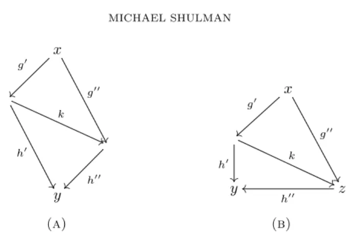
Here by thecategory of factorizationsof a morphism f :x→y, we mean the category whose objects are pairs of morphisms (h, g) such that hg=f, and
whose morphisms (h, g) → (h0, g0) are morphisms k (which we call connecting morphisms) such thatg0 =gk andh=h0k:
h
k
g ??
g0 h0
?
?
The statement (∗) is about the full subcategory of this on the objects (h, g) such that dom(h) = cod(g) lies inC.
Proof. By definition, the functor [α]→ E is bijective on objects, and fully faithful except possibly between objects ofD. Ford, d0∈ D, the map [α](d, d0)→ E(d, d0) has two components, one of which is the inclusionD(d, d0),→ E(d, d0), and the other of which is the map
(6.11) E( –, d0)⊗CE(d,– )→ E(d, d0).
Now by definition,E( –, d0)⊗CE(d,– ) is the quotient of the set`c∈CE(c, d0)× E(d, c)
by the equivalence relation generated by setting (h, kg)∼(hk, g) for anyg:d→c,
k:c→c0, andh:c0 →d0, and (6.11) is induced by composition. Thus, the first clause of condition (∗) ensures that the two components of [α](d, d0)→ E(d, d0) have disjoint images and are jointly surjective. Moreover, the preimage of f : d→d0
under (6.11) is the quotient of the set of factorizations (h, g) of f by this same relation. This is exactly the relation generated by morphisms in the category of factorizations, so the second clause of (∗) ensures that the second component of [α](d, d0)→ E(d, d0) is injective (the first component being obviously so). Another way to state this is: consider the collection of morphisms between objects not inC that do not factor through any object ofC. If these morphisms contain the identities and are closed under composition, they form a non-full subcategory
D. In this case, we can defineU,W, andαas above, and the only remaining part of (∗) to check is that if a morphism between objects of Dfactors throughC then the category of such factorizations is connected.3
This leads to a recognition principle for bistratified categories. First we state some definitions.
Definition 6.12. LetC be a category whose objects are assigned ordinal degrees.
• A morphism islevelif its domain and codomain have the same degree.
• The degree of a factorization (h, g) of a morphism f is the degree of the intermediate object dom(h) = cod(g).
• A factorization of a morphismf isfundamentalif its degree is strictly less than the degrees of both the domain and codomain off.
• A morphism isbasicif it does not admit any fundamental factorization. Theorem 6.13. A categoryC whose objects are assigned ordinal degrees is bistrat-ified if and only if the following conditions hold.
(i) All identities are basic.
(ii) Basic level morphisms are closed under composition.