Weld Distortion Prediction With Virtual Analysis For Practical Applications

University of Windsor University of Windsor

Scholarship at UWindsor

Scholarship at UWindsor

Electronic Theses and Dissertations Theses, Dissertations, and Major Papers

2014

Weld Distortion Prediction With Virtual Analysis For Practical

Weld Distortion Prediction With Virtual Analysis For Practical

Applications

Applications

Francesca Folchi University of Windsor

Follow this and additional works at: https://scholar.uwindsor.ca/etd

Recommended Citation Recommended Citation

Folchi, Francesca, "Weld Distortion Prediction With Virtual Analysis For Practical Applications" (2014). Electronic Theses and Dissertations. 5229.

https://scholar.uwindsor.ca/etd/5229

This online database contains the full-text of PhD dissertations and Masters’ theses of University of Windsor students from 1954 forward. These documents are made available for personal study and research purposes only, in accordance with the Canadian Copyright Act and the Creative Commons license—CC BY-NC-ND (Attribution, Non-Commercial, No Derivative Works). Under this license, works must always be attributed to the copyright holder (original author), cannot be used for any commercial purposes, and may not be altered. Any other use would require the permission of the copyright holder. Students may inquire about withdrawing their dissertation and/or thesis from this database. For additional inquiries, please contact the repository administrator via email

WELD DISTORTION PREDICTION WITH VIRTUAL

ANALYSIS FOR PRACTICAL APPLICATIONS

By

FRANCESCA FOLCHI

A Thesis

Submitted to the Faculty of Graduate Studies

through the Department of Mechanical, Automotive and Material Engineering in Partial Fulfillment of the Requirements for

the Degree of Master of Applied Science at the University of Windsor

Windsor, Ontario, Canada

2014

WELD DISTORTION PREDICTION WITH VIRTUAL

ANALYSIS FOR PRACTICAL APPLICATIONS

by

Francesca Folchi

APPROVED BY:

______________________________________________ R. Bowers

Department of Mechanical, Automotive & Materials Engineering

______________________________________________ D. Ting

Department of Mechanical, Automotive & Materials Engineering

______________________________________________ V. Stoilov, Advisor

Department of Mechanical, Automotive & Materials Engineering

iii

DECLARATION OF ORIGINALITY

I hereby certify that I am the sole author of this thesis and that no part of this thesis has been published or submitted for publication.

I certify that, to the best of my knowledge, my thesis does not infringe upon anyone’s copyright nor violate any proprietary rights and that any ideas, techniques,

quotations, or any other material from the work of other people included in my thesis, published or otherwise, are fully acknowledged in accordance with the standard referencing practices. Furthermore, to the extent that I have included copyrighted material that surpasses the bounds of fair dealing within the meaning of the Canada Copyright Act, I certify that I have obtained a written permission from the copyright owner(s) to include such material(s) in my thesis and have included copies of such copyright clearances to my appendix.

iv

ABSTRACT

v

DEDICATION

vi

ACKNOWLEDGEMENTS

First of all, I would like to thank my advisors Dr. Vesselin Stoilov and Prof. Giovanni Belingardi for their useful suggestions and remarks through the difficult thesis process. I would like also to thank my committee members, Dr.Randy Bowers and Dr. David Ting.

I would like to express my appreciation to my Chrysler tutor Greg Medler and my Chrysler supervisor Mohammed Malik for the assistance provided. A special thank goes to Jeffrey Stewart from the Chrysler Welding group for the big help provided in the weld lab.

It has been a year full of emotions and for this reason I would like to thank all the amazing people that helped me through this journey:

First of all, my friends Giuseppe, Marco, Federico, the two Luca, Ashley, Tom, Kyle, Felicia, Steven, Antonio and Kathleen for the great times spent together here in Windsor.

All my Italian friends, for reminding me that friendship is stronger than distance.

My best friend, sister and “snowflake”, Marianna, for the amazing support that she gave

me through these years, she has always been beside me in every adventure.

My boyfriend and best friend, Nicola, for standing by my side in every choice I made.

My grandmother and my uncles, in particular Zia Patrizia for her unconditional support.

I want to reserve the most important thank to my parents, Enzo and Flora, for believing in me and for being my guide.

vii

TABLE OF CONTENTS

DECLARATION OF ORIGINALITY ... iii

ABSTRACT ... iv

DEDICATION ... v

ACKNOWLEDGEMENTS ... vi

LIST OF TABLES ... x

LIST OF FIGURES ... xii

LIST OF APPENDICES ... xvi

LIST OF ABBREVIATIONS/SYMBOLS ... xvii

NOMENCLATURE ... xviii

CHAPTER 1 INTRODUCTION AND LITERATURE REVIEW ... 1

1.1 Introduction ... 1

1.2 Literature Review ... 2

1.2.1 Numerical simulation approach ... 2

1.2.2 Statistical approaches ... 13

1.2.3 Empirical approach ... 15

1.2.4 Industrial relevance for welding distortion prediction ... 16

CHAPTER 2 THEORY BEHIND WELD DISTORTION AND NUMERICAL APPROACH ... 18

2.1 Theory behind weld distortion ... 18

2.1.1 Fundamentals and general technology of welding... 18

2.1.2 Complex coupling in welding modeling ... 24

2.1.3 Residual stresses and distortions calculations ... 34

viii

CHAPTER 3 EXPERIMENTAL SETUP ... 41

3.1 Definition of geometry and welding process parameters ... 41

3.2 Distortion measurement ... 44

3.3 Results and discussion ... 45

CHAPTER 4 NUMERICAL SIMULATION OF ARC WELDING ... 49

4.1 Model development for Transient analysis-SYSWELD ... 50

4.2 Model development for Shrinkage method-WELD PLANNER ... 53

4.3 Results and discussions for transient analysis-SYSWELD ... 55

4.4 Results and discussion for shrinkage method- WELD PLANNER ... 66

4.5 Validation of transient analysis and shrinkage method with data from the literature review... 68

4.5.1 Model development and results for transient analysis-SYSWELD .. 69

4.5.2 Model development and results for shrinkage method - WELD PLANNER 72 4.5.3 Comparison between transient and shrinkage analysis approach for the validation test ... 76

CHAPTER 5 COMPARISON BETWEEN NUMERICAL RESULTS AND EXPERIMENTAL RESULTS... 78

5.1 Comparison between transient analysis results and experimental results 78 5.2 Comparison between shrinkage method and experimental results ... 87

CHAPTER 6 OPTIMIZATION WITH WELD PLANNER ... 88

CHAPTER 7 CONCLUSIONS AND RECOMMENDATIONS ... 95

7.1 Conclusions ... 95

7.2 Future work and recommendations ... 96

APPENDICES ... 98

ix

Appendix B - A guide to welding process in WELD PLANNER ... 106

Appendix C- Wire filler properties ... 110

REFERENCES ... 111

x

LIST OF TABLES

Table 1.1- Comparison between the common modeling-optimization techniques [26] ... 15

Table 3.1- Coupon dimensions ... 41

Table 3.2- Requirements for Chemical Composition(% by Mass) of MS 67 ... 42

Table 3.3- Minimum Mechanical properties of mild steels in transverse direction- Chrysler standard for MS 67 ... 42

Table 3.4- Minimum Mechanical Properties of high strength steel MS 264 05 XK in transverse direction ... 42

Table 3.5- Welding parameters ... 42

Table 3.6- Materials and clamping condition used for the six tests ... 43

Table 3.7-Distance results [mm] in experimental tests ... 46

Table 3.8-Displacement [mm] in experimental tests ... 46

Table 4.1- Chemical composition (%by mass) of low carbon steel S355J2G3-EN 10025 [21] ... 51

Table 4.2-Minimum Mechanical Properties of S355J2G3 (EN 10025) or st52(DIN 17100) [21] [57] ... 51

Table 4.3-Chemical composition (% by mass) for plain carbon steel DC 04-AISI 1006 [58] ... 51

Table 4.4-Minimum Mechanical properties of DC 04-AISI 1006 ... 51

Table 4.5- Heat source parameters used in the simulations ... 52

Table 4.6-Simulation measurement [mm] and displacement [mm] results for T-joint Test #1... 56

Table 4.7- Simulation measurement [mm] and displacement [mm] results for T-joint Test #2... 57

Table 4.8- Simulation measurement [mm] and displacement [mm] results for T-joint Test #3... 59

Table 4.9- Simulation measurement [mm] and displacement [mm] results for T-joint Test #4... 60

Table 4.10- Simulation measurement [mm] and displacement [mm] results for T-joint Test #5 ... 62

Table 4.11- Simulation measurement [mm] and displacement [mm] results for T-joint Test #6 ... 63

Table 4.12-Von Mises stress [MPa] among the six tests and relative average value and standard deviation ... 66

Table 4.13-Welding parameters used in Sulamain et al. research ... 68

Table 4.14-Experimental results of the validation test ... 69

Table 4.15- Heat source parameters used in the simulation for validation ... 70

xi

Table 4.17- Comparison of Angular distortion results [mm] between simulation and experiment for t-joint validation case (WELD PLANNER) ... 75 Table 4.18- Comparison between transient analysis results and shrinkage analysis results for t-joint for the validation test ... 76 Table 5.1- Displacement results and error between simulation and experimental results for Test #1 ... 78 Table 5.2- Average errors along the lines for Test #1 ... 78 Table 5.3-- Displacement results and error between simulation and experimental results for Test #2-uncontrolled condition ... 80 Table 5.4- Average errors along the lines for Test #2 ... 80 Table 5.5-- Displacement results and error between simulation and experimental results for Test #3-uncontrolled condition ... 81 Table 5.6- Average errors along the lines for Test #3 ... 81 Table 5.7-- Displacement results and error between simulation and experimental results for Test #4-uncontrolled condition ... 82 Table 5.8- Average errors along the lines for Test #4 ... 83 Table 5.9-- Displacement results and error between simulation and experimental results for Test #5-uncontrolled condition ... 84 Table 5.10- Average errors along the lines for Test #5 ... 84 Table 5.11-- Displacement results and error between simulation and experimental results for Test #6-uncontrolled condition ... 85 Table 5.12- Average errors along the lines for Test #6 ... 86 Table 6.1-Material combination for Case #1 and Case #2 ... 88 Table 6.2-Influence of thickness on the maximum displacement in case of arc bead width of 5 mm ... 90 Table 6.3- Influence of thickness on the maximum displacement in case of arc bead width of 6 mm ... 90 Table 6.4- Influence of thickness on the maximum displacement in case of arc bead width of 6.8 mm ... 90 Table 6.5-Maximum displacement results for base clamping configuration and

configuration A ... 93 Table 6.6-Maximum displacement results for base clamping configuration and

xii

LIST OF FIGURES

Figure 1.1- Longitudinal shrinkage in 2.5mm and 3 mm thick plate [4] ... 3

Figure 1.2- Longitudinal shrinkage in 2.5mm and 3 mm thick plate [4] ... 4

Figure 1.3- Example of optimization [13] ... 7

Figure 1.4-Full transient analysis (displacements) [20] ... 9

Figure 1.5-Shrinkage analysis (displacement) [20] ... 10

Figure 1.6-Comparison of distortion in the transient model and in the shrinkage model [12] ... 11

Figure 1.7-Example of the procedure for setting up welding models: (a) shrinkage analysis; (b) transient analysis [12] ... 12

Figure 1.8-Developed ANN architecture for the residual stress prediction [24] ... 14

Figure 1.9- Share of lightweight materials in aviation, wind and automotive field [30] .. 17

Figure 1.10-Illustration of door hinge assembly [33] ... 17

Figure 2.1- Principal zones in a cross section of a welded joint [35] ... 19

Figure 2.2- Basic arc welding configuration [36] ... 19

Figure 2.3- Gas metal arc welding (GMAW) basic configuration [35] ... 21

Figure 2.4-Gas tungsten arc welding (GTAW) [35] ... 22

Figure 2.5-(a) Butt joint, (b)Corner joint and (c) Lap joint [35] ... 23

Figure 2.6- (d) Tee joint and (e) Edge joint [35] ... 23

Figure 2.7- Different types of welding distortion [11] ... 25

Figure 2.8-Coupling welding process [39] ... 26

Figure 2.9- Double ellipsoid heat source [44] ... 27

Figure 2.10- Variation of material properties with the temperature for 5052-H32 aluminum alloy (a) thermal properties, (b) mechanical properties [47] ... 30

Figure 2.11- Body centered cubic crystal structure [49]- α phase ... 31

Figure 2.12-Face centered cubic crystal structure [49]-γ phase ... 32

Figure 2.13- HAZ and equilibrium diagram [50] ... 32

Figure 2.14-Example of visual appearance of hydrogen cracking [51] ... 33

Figure 2.15- Strain gauge rosette [52] ... 35

Figure 2.16- Bonded metallic strain gauge [56] ... 38

Figure 2.17-Models of shrinkage forces and moments for butt joint (left) and T-Joint (right) [21] ... 40

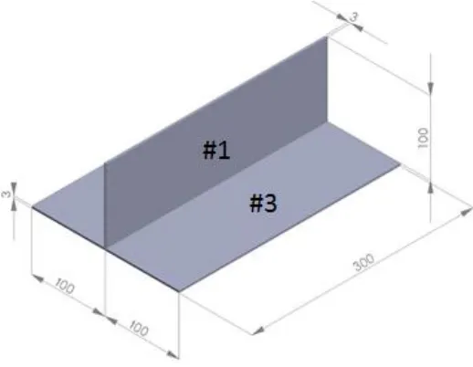
Figure 3.1- Tee joint geometry- measurements in mm ... 41

Figure 3.2-T-joint setup ... 44

Figure 3.3- Position of 12 Points on Coupon#3-Top view ... 45

Figure 3.4-Position of the 6 points on Coupon #1 and 12 distances measured (in red) ... 45

Figure 3.5-Experimental displacement [mm] for Test #1 and Test #2 ... 47

Figure 3.6- Experimental displacement [mm] for Test #3 and Test #4 ... 48

Figure 3.7- Experimental displacement [mm] for Test #5 and Test ... 48

xiii

Figure 4.2- T-joint mesh for transient analysis ... 50

Figure 4.3- Software section (left) and real section (right) of the T-joint for transient analysis ... 50

Figure 4.4- 3D skin for cooling condition ... 52

Figure 4.5-Position of the clamps for simulation Test#3 and Test #4 ... 53

Figure 4.6- T-joint mesh for controlled clamping condition ... 54

Figure 4.7- T-joint filler geometry in WELD PLANNER ... 54

Figure 4.8-Clamping condition for Test #3 WELD PLANNER ... 55

Figure 4.9- Weld Plan T-joint for simulation Test #3 and Test#4 in WELD PLANNER 55 Figure 4.10-Displacement [mm] trend in z-direction obtained with transient analysis for T-joint Test #1... 56

Figure 4.11-Von Mises stress [MPa] trend obtained with transient analysis for T-joint Test #1 ... 57

Figure 4.12- Displacement [mm] trend in z-direction obtained with transient analysis for T-joint Test #2... 58

Figure 4.13- Von Mises Stress [MPa] trend obtained with transient analysis for T-joint Test #2 ... 58

Figure 4.14- Displacement [mm] trend in z-direction obtained with transient analysis for T-joint Test #3... 59

Figure 4.15- Von Mises Stress [MPa] trend obtained with transient analysis for T-joint Test #3 ... 60

Figure 4.16- Displacement [mm] trend in z-direction obtained with transient analysis for T-joint Test #4... 61

Figure 4.17- Von Mises Stress [MPa] trend obtained with transient analysis for T-joint Test #4 ... 61

Figure 4.18- Displacement [mm] trend in z-direction obtained with transient analysis for T-joint Test #5... 62

Figure 4.19- Von Mises Stress [MPa] trend obtained with transient analysis for T-joint Test #5 ... 63

Figure 4.20- Displacement [mm] trend in z-direction obtained with transient analysis for T-joint Test #6... 64

Figure 4.21- Von Mises Stress [MPa] trend obtained with transient analysis for T-joint Test #6 ... 64

Figure 4.22-Comparison between simulation displacements between Test #1 and Test #2 ... 65

Figure 4.23- Comparison between simulation displacements between Test #3 and Test #4 ... 65

Figure 4.24- Comparison between simulation displacements between Test #5 and Test #6 ... 66

xiv

Figure 4.26- Distortion [mm] in z-direction [mm] for Test #3 and Test #4 ... 67

Figure 4.27- Distortion [mm] in z-direction [mm] for Test #5 and Test #6 ... 67

Figure 4.28- T-joint clamping condition [21] ... 69

Figure 4.29- T-joint mesh for the t-joint validation test ... 70

Figure 4.30-Software section (left) and real section (right) of the T-joint validation test 70 Figure 4.31- Displacement [mm] trend in z-direction for t-joint validation test at 3600s (view of the 1st welded side) ... 71

Figure 4.32- Displacement [mm] trend in z-direction for t-joint validation test at 3600s (view of the 2nd welded side) ... 71

Figure 4.33- Von Mises stress [MPa] for T-join validation test at 3600s ... 72

Figure 4.34-T-joint mesh validation test ... 73

Figure 4.35-T-joint filler geometry-validation test ... 73

Figure 4.36-CLAMP_01 and CLAMP_02 position... 74

Figure 4.37-Weld Plan t-joint validation test ... 74

Figure 4.38-Displacement [mm] in z-direction t-joint validation test(WELD PLANNER) ... 74

Figure 4.39- Magnification 10x of the deformed T-joint validation case (WELD PLANNER) ... 75

Figure 4.40- Qualitative distortion trend comparison between transient analysis (left) and shrinkage analysis (right) for the first welded side ... 77

Figure 4.41- Qualitative distortion trend comparison between transient analysis (left) and shrinkage analysis (right) for the second welded side ... 77

Figure 5.1- Displacements T-joint Test#1 for uncontrolled clamping condition ... 79

Figure 5.2- Displacements T-joint Test#2 for uncontrolled clamping condition ... 80

Figure 5.3- Displacements T-joint Test#3 for uncontrolled clamping condition ... 82

Figure 5.4- Displacements T-joint Test#4 for uncontrolled clamping condition ... 83

Figure 5.5 -Displacements T-joint Test#5 for uncontrolled clamping condition ... 85

Figure 5.6- Displacements T-joint Test#6 for uncontrolled clamping condition ... 86

Figure 5.7-Example of distance for transient analysis model (left) and shrinkage analysis model (right) ... 87

Figure 6.1-Geometry and dimensions of the T-joint used for the optimization ... 88

Figure 6.2-Base Clamping configuration for both Case #1 and Case #2 ... 89

Figure 6.3-Different arc bead widths used in the simulations ... 89

Figure 6.4-Influence of different arc bead width on Max Displacement ... 91

Figure 6.5-Influence of different material thicknesses on maximum displacement ... 92

Figure 6.6- Difference between base clamping configuration and clamping configuration A ... 93

Figure 6.7- Difference between base clamping configuration and clamping configuration B ... 94

xv

Figure 8.2-Example of Step1-Project description ... 99

Figure 8.3-Different types of welding processes included in Welding Advisor ... 100

Figure 8.4- Trajectory and reference path using for the moving heat source ... 101

Figure 8.5-Parameters require for the welding process (Step 4) ... 101

Figure 8.6- Penetration, width and length of the heat source ... 102

Figure 8.7-Example of cooling condition (Step 5) ... 102

Figure 8.8-Example of Clamping Condition (Step 6) ... 103

Figure 8.9-Example of Step 7 and Step 8 ... 103

Figure 8.10-Example of Solution Parameter (Step 9) ... 104

Figure 8.11-Contours definition... 105

Figure 8.12-Weld Planner workflow [60] ... 106

Figure 8.13-Example of material database in Weld Planner ... 107

Figure 8.14-Example of weld parameters in Weld Planner ... 107

Figure 8.15-Example of clamping definition in Weld Planner ... 108

Figure 8.16-Example of weld plan definition in Weld Planner ... 108

xvi

LIST OF APPENDICES

Appendix A - A guide to welding process in Sysweld Environment ………98

Appendix B - A guide to welding process in WELD PLANNER………...106

xvii

LIST OF ABBREVIATIONS/SYMBOLS

ANN Artificial Neural Network

AW Arc Welding

DOE Design of Experiment EGW Electro-gas Welding

EW End of Welding

FCAW Flux-Cored Arc Welding FEM Finite Element Method GA Genetic Algorithm, GMAW Gas Metal Arc Welding GTAW Gas Tungsten Arc Welding HAZ Heat Affected Zone PAW Plasma Arc Welding

xviii

NOMENCLATURE

̅ Phase proportion after an infinite time at temperature T Heat transfer coefficient

Cross sectional area Sum of the body forces Heat energy per unit length Material strain hardening Arc resistance

Reference temperature

Surface temperature Ambient temperature Volume of the heat source Specific heat

Fraction of heat deposited in the front

Fraction of heat deposited in the rear

Number of divisions in the welding

̅ Phase proportion obtained at an infinitely low temperature

Conduction heat Convective heat

Front heat flow

Rate of internal heat generation Rear heat flow

Radiation heat

Welding speed Transverse shrinkage Emissivity

Elastic strain vector Plastic strain vector

xix Stefan-Boltzman constant Longitudinal residual stress Transverse residual stress

Cauchy stress tensor

Delay time

D Material stiffness matrix

E Elastic modulus

F Equivalent shrinkage force

I Welding current

K Thermal conductivity

K Equivalent shrinkage stiffness

L Length of the weld seam

M Equivalent bending moment

n Exponent related to the reaction speed

p Phase proportion

Q Electrical energy consumed

r Initial root gap

s Thickness of the plate

T Temperature

v Poisson ration

V Voltage

x Shrinkage value

z Unfused depth of root

η Efficiency of heat source

Increment of plastic strain

Increment of yield strength Thermal expansion

Strain vector Angular distortion Density

1

1 CHAPTER 1

INTRODUCTION AND LITERATURE REVIEW

1.1 Introduction

Prediction of weld distortion has become an important issue in many manufacturing processes. The prediction of the weld distortion can partially or fully eliminate the post processes needed to mitigate the distortion. In this way, an early stage of study of the distortion can lead to a reduction in manufacturing costs due to extra labor time and facilities consumption. The disadvantage of post welding correction is to add another work step that decreases the productivity.

In the arc welding process, the heat is used to fuse the metal, and filler can be added to the molten pool in order to join two or more parts. The heating and the consequent cooling cycles of this process lead to a non-uniform contraction and expansion of the material. Three main zones can be distinguished after the welding process: the base metal, the weld metal and the heat affected zone. The base metal is not involved in the welding process and it remains near room temperature, whereas fusion zone is the part of the metal that completely melted by the welding heat. During the cooling process, the weld metal contracts to the volume it occupied at room temperature. This contraction is limited by the base metal, which acts as a holding vice. For this reason the weld deposit tends to accumulate tensile stresses, which can cause distortion. The mechanical behavior of welds is strongly related to the heat transfer, the microstructure evolution and thermal stress. As a consequence, the theory behind welding is very complex and difficult to fully understand. Mechanical, metallurgical and thermal analyses are key factors that need to be studied in order to understand the complex coupling of the welding process.

2

linear thermal contraction without the need of temperature and phase transformation material properties.

The main goal of this research is to provide a quick prediction of weld distortion. The objectives focus on the development of a model of distortions after arc welding and validation of the results obtained in virtual analysis with experimental data and data found in the open literature.

1.2 Literature Review

The changes in mechanical, metallurgical and thermal properties of the material characterized the complex coupling of the welding process. Welding is a complex non-linear process that presents a significant challenge to theoretical description [1]. In order to predict the distortion of the material after welding, different methods can be applied. Some of these methods are direct numerical simulation, statistical, empirical and semi-empirical models, and experimental characterization.

1.2.1 Numerical simulation approach

Numerical simulation can be divided into the following categories:

 Transient analysis;  Shrinkage analysis;  Local-global analysis.

1.2.1.1 Transient analysis

The most complex and advanced level of simulation is the transient analysis because physical phenomena such as shape, size, heat source, melt pool and metal, temperature and rate-dependent phase transformation and material properties are required in order to evaluate the distortion and the final microstructure of the metal.

ABAQUS Finite element analysis

3

found in the analysis of the arc welding induced residual stresses in butt-joint by Kohandehghan and Serajzadeh [3], where two different conditions including unconstrained and constrained simulations were performed. The simulation results were compared with experimental data showing good correlations. The results showed how constraints affect the thermal and the mechanical response of the plate and how they influenced the final distortion. Long et al. [4] investigated the longitudinal and transverse distortions on a butt joint GMAW welding of a thin plate, using a double-ellipsoid moving heat source with ABAQUS software. The results showed that the FE simulations were able to predict the distortions reasonably well compared to the experimental results. High values of longitudinal shrinkage were found in the weld rather than in the outer rim of the plate (Figure 1.1) and the longitudinal shrinkage increased with the decreasing welding speed.

Figure 1.1- Longitudinal shrinkage in 2.5mm and 3 mm thick plate [4]

4

Figure 1.2- Longitudinal shrinkage in 2.5mm and 3 mm thick plate [4]

As for the longitudinal and transverse shrinkages, both increased with lower welding speeds. In general it was observed that the FE simulation yields better results at higher speeds. This can be attributed to the use of the same heat source parameters with different welding speeds and also to the lack of details of the material properties. The simulation slightly underestimated the distortion, whereas the empirical predictions (Section 1.2.3) showed a significant underestimation.

5

mechanical analysis plane strain quasi static finite element analyses were accomplished using quadrilateral elements; the mesh was the same as the one in the thermal analysis. The residual stress field from thermal simulation is applied as a load in the mechanical analysis. Results were compared with the experimental data, and in general good agreement is achieved with only the exception of the temperature in the weld region. This behaviour can be attributed to the two dimensional model that does not take into account the heat flow in the welding direction. The plain strain assumption was confirmed by the experimental results that showed that the residual stresses were independent from the panel size. The critical buckling load was compared to the applied load using continuum and structural models in the three finite element methods. At the end, the decoupling of the weld simulation was showed to be efficient and time saving; it also allowed quick changes of the geometries.

Even though ABAQUS has the ability to provide an accurate welding simulation, the building of the model and consecutive calculations require significant amount processing time. For instance, an 80 pass welding simulation using ABAQUS would require a setup of 240 steps, with the assumption of 3 steps per pass, and the need to insert all the step time and initial temperatures. The amount of data required for the setup of the inputs is significant. For this reason, the Abaqus Welding Interface (AWI) is available as an ABAQUS/CAE plug-in. It improves the two-dimensional welding simulations; moreover the setup time for the previous example of an 80 pass model is approximately one hour compared to days with the standard simulation [6].

ANSYS-Finite Element Analysis

6

welding assembly on auto-body high-strength steel panel and door hinge [8]. In this study, moving ellipsoid heat source and birth-death element method were used in order to obtain the complex transient temperature distribution and the mechanical residual stresses. The simulation showed good agreement and the method was used to optimize a number of parameters. In Sattari-Far’s research [9], the ANSYS software was used to determine the effect of nine different welding sequences on an AISI 304 stainless steel pipe. In the 3D modeling, birth-death element method was introduced, whereas in the experimental model, the diameters of the pipes were measured before and after the welding. In order to find a suitable and more appropriate welding sequence, two criteria were introduced: the maximum diameter variation and the average diameter variation. The results showed that the simulation results were in good agreement with the experimental results. The pipe diameter distortions were negative within the weld zone and became positive far from the welding center line. In this research it is observed that a welding sequence made of four segments can lead to higher distortions compared to a two segment welding sequence.

VRWELD

Software called VRWELD is able to simulate the transient behavior of the temperature and the microstructure evolution after the welding process. A validation of this software was conducted by Goldak and Asadi [10]. They compared the results of the simulation conducted with VRWELD with the experiments conducted by Masabuchi [11].

SYSWELD

7

Figure 1.3- Example of optimization [13]

The phase composition can be easily simulated with the input of the phase-dependent material properties. Even though this is the most accurate software in the welding distortion field, the time required to model large assemblies can be enormous. In order to decrease the time of the simulation different strategies can be applied. For example, in Feulvarch’s research [14], multi-pass welding was simulated with SYSWELD in 2D and

8

simulation, such as welding speed, welding current, welding voltage and thickness. The results showed that the effect of the welding speed was the most influential compared to the other parameters.

In welding there is a strong coupling between thermodynamics, mechanics and microstructure properties. For this reason Heinze et al. [16] studied the thermal model using experimental data to configure equivalent heat sources which were input for the thermal model. The work concentrated on the equivalent heat sources such as conical Gauss or double-ellipsoid Goldak heat source. SYSWELD was used to run the simulations, varying the heat source parameters and the thermal conductivity. In addition, this software made it possible to introduce the metallurgical phase transformation in the simulation. Even though the pulsed GMA welds led to complex weld pool shapes, the challenge of this characteristic could be overcome using SYSWELD to simulate the experimental weld geometry.

In the research of Lidam et al. [17], the angular distortion analysis of a multipass welding process on combined joint types was studied using SYSWELD. The multipass welding advisor included in SYSWELD was used to evaluate the angular distortion produced by GMAW process. The goal of the research was to analyze the angular distortion of a combined butt and t-joint using SYSWELD and experimental results. The experiments were carried using a fully automated welding process with GMAW power source and shielding gas composition of Ar/CO2 (80/20). The specimen of low carbon steel was clamped during the whole welding process.

The experiments were simulated with 2D and 3D models and an extensive study was made in order to calibrate the heat source of the GMAW to be equal to the molten zone of the specimen. The angular distortion was calculated using a coordinate measuring machine, and measurements were conducted before and after the welding process at 12 different points. Based on the results, the 3D model showed better correlation with an error of 14-17% compared with the 2D model with an error of 38-40%. On the other hand, the 2D simulation was significantly faster (20 min) compared with the 3D simulation (30hrs).

9

the effect of the clamp releasing time on angular distortion and residual stresses. Three different clamping conditions were evaluated: unclamped, clamped until the end of the welding process and clamped until cool down at ambient temperature. The analysis showed that the clamping condition with cold release induces less distortion compared to the other clamping conditions, but at the same it increases the residual stresses.

1.2.1.2 Shrinkage approach

The shrinkage volume approach is the fastest and least complex method due to the fact that neither temperature nor phase dependent material data are required for the prediction of the welding distortion [12]. The shrinkage approach assumes that a linear thermal contraction is responsible for the distortion; the elements shrink with a value that is equal and opposite to the thermal expansion that would have occurred if the material was heated up to its melting temperature [12] [19]. This method is useful in the design stage of welded parts because it is less time consuming compared to the transient analysis. The software WELD PLANNER is dedicated to identify distortions, critical weld joints, clamping conditions and weld sequences using the shrinkage method [20]. ESI group compared the full transient analyses and the shrinkage method in a T-joint configuration [20]. The transient simulation had similar level of distortion compared to the shrinkage method [20] as shown in the Figure 1.4 and Figure 1.5.

10

Figure 1.5-Shrinkage analysis (displacement) [20]

11

12

Figure 1.7-Example of the procedure for setting up welding models: (a) shrinkage analysis; (b) transient analysis [12]

13

1.2.1.3 Local-global analysis

Distortion prediction in large structures can be very difficult; for this reason, the projection method is introduced. It consists of studying the global process starting from a smaller sub-process. If this procedure is composed of two length scales, the method is called local-global analysis [22]. The model consists of applying the distortions found in the local simulation in the whole structure. This approach is implemented in the PAM-ASSEMBLY software. It has the advantage of reducing the simulation time compared to the full transient analysis. However, it still requires SYSWELD for the simulation of the local analysis [12].

1.2.2 Statistical approaches

Various methods can be used to define the input values required to produce the desired output variables through the development of mathematical models. Surrogate models can be used when the output cannot be easily calculated. In the field of welding distortion, the surrogate models can help to avoid the non-linearity of the process. In addition, this type of model can decrease the simulation time and find the solution with all the possible combinations. Surrogate models were studied by Goldak and Asadi [23]. They demonstrated how a model was able to minimize the distortion in a girth weld of a pipe with 6 sub-passes by analyzing just 14 sequences.

14

Figure 1.8-Developed ANN architecture for the residual stress prediction [24]

Tian et al. [25] developed an ANN model to predict the transverse and angular distortion of an S304 material using gas-tungsten arc welding. The experiments were bead-on-plate welds. The angular and transverse distortions were calculated across a certain range of welding parameters. Additionally a finite element method was developed in ABAQUS. The simulation consisted of a step of non-linear transient thermal analysis and a step of temperature history needed to calculate the distortion. The results showed the non-linearity between the input welding parameters and the final distortion. For this reason, an artificial neural network was used to solve the non-linearity problem. A BP network, which consists of one or more hidden layers and an output layer, was used and trained using a Matlab Toolbox. The accuracy of the BP network was verified by comparison to the experimental results with a correlation coefficient of 0.99.

15

Table 1.1- Comparison between the common modeling-optimization techniques [26]

1.2.3 Empirical approach

In the literature review, it is possible to find empirical equations that approximate the longitudinal and transverse distortion already discussed in the paragraph 2.2.

For the transverse shrinkage, Sparagen [27] introduced an empirical equation for a butt weld:

(1.1)

where is the cross sectional area of the weld, is the thickness of the plate and r is the initial root gap .

For a single pass butt weld White [28] developed the following equation:

( ) ( ₎

(1.2)

where z is the unfused depth of root, is the thickness of the plate, Q (J) is

the energy, ( ) is the welding speed. The previous equation 1.2 can be

16

Another example of transverse shrinkage is given by Capel’s formula [11](Equation 1.3) calculated on butt welds in 6.4mm thick plate for carbon steels:

(1.3)

where is the thickness of the plate and ( ) is the welding speed. As for the

longitudinal shrinkage, Okerblom [29] introduced the formula (Equation 1.4) for the distortion prediction in case of fast welding speeds:

(1.4)

where is the coefficient of thermal expansion , is the specific heat, ( ) is the

welding speed and is the thickness of the plate. In Long’s research [4], the empirical results showed considerable underestimation of the welding distortion compared to the FE simulations.

1.2.4 Industrial relevance for welding distortion prediction

The use of lightweight structures is a key point in the reduction of fuel consumption and operating costs in automotive and ship building industries. The use of lightweight materials is widely shared in aviation field. It will grow significantly in the automotive field from 30 to 70 percent by 2030, as it is possible to observe in the Figure 1.9 [30].

17

Figure 1.9- Share of lightweight materials in aviation, wind and automotive field [30]

According to Volkswagen, the use of software for welding prediction can save one or two potential loops, meaning 10-20 k€ per part reduction [32]. In automotive assembly, doors are assembled to auto-body side-frame through hinges by GMAW (Figure 1.10). Distortion of the hinges can seriously affect the position of the door, which can lead to poor sealing and abnormal sounds during closing and opening [8].

18

2 CHAPTER 2

THEORY BEHIND WELD DISTORTION AND NUMERICAL APPROACH

2.1 Theory behind weld distortion

2.1.1 Fundamentals and general technology of welding

Welding is a process in which two parts can be joined together at their contact surface using heat and/or pressure. Welding is widely employed in fabrication due to its good reliability, cost-effectiveness and high efficiency [25]. The welded joint can be stronger than the parental metal, and it is an economical way to join materials. In theory, continuity between the two parts should be observed, and the joint area should be indistinguishable from the parent metal of the individual parts [34]. Unfortunately, the ideal conditions cannot be achieved. For this reason, different types of welds should be performed for different materials. In some welding processes, filler is added in order to facilitate the coalescence of the two materials. However, there are some drawbacks in welding processes, such as the high energy required, inconvenient disassembly and quality defects in welded joints.

The welding process can be divided in two categories: fusion welding and solid state welding. The former one is the most important and widely used category and includes arc welding, resistance welding, oxy-fuel gas welding processes.

In fusion welding, the heat is used to fuse the metal; and usually filler is added to the molten pool to facilitate the process and provide bulk and strength to the welded joint [35]. The fusion welded point consists of three different zones (Figure 2.1):

19

2. Weld interface: the boundary that divides the fusion zone from the heat-affected zone. This interface is relatively thin due to the fast solidification that occurred before any mixing with the metal in the fusion zone;

3. Heat-affected zone (HAZ): in this zone the metal has experienced temperatures that are below its melting point, but were high enough to cause a microstructural changes inside the solid metal [35].

Figure 2.1- Principal zones in a cross section of a welded joint [35]

Arc welding (AW) is a fusion welding process where two parts are coalesced using an electric arc between an electrode and the work pieces. The electric arc is a discharge of current across a gap in a circuit, it is sustained by the presence of a thermally ionized column of gas (plasma) through which a current flows [35].

20

Two types of electrodes are used in arc welding: consumable electrodes and non-consumable electrodes. The former ones provide filler metal during the process; because they are consumable, they need to be changed during the weld process. The latter ones are made with tungsten which resists melting during the operation; in this case the filler has to be supplied separately.

Another important feature in arc welding is the arc shielding. At high temperatures, molten metal is chemically reactive with the surrounding air, which can negatively affect the quality of welding. For this reason, the electrode tip, arc and molten pool have to be covered with a blanket of flux or gas to prevent the exposure of the molten metal with the air [35].

The energy supplied by the power supply to the electrode is directly proportional to the welding current [34] as can be obtained by the equations 2.1 and 2.2:

(2.1)

(2.2)

where Q is the electrical energy consumed ⁄ , I is the welding current (A), V is arc voltage (V) , and is the arc circuit resistance (Ω). The welding current plays an important role in the quality of the welding because it affects the electrode melting rate and enhances the deposition rate, the depth of the penetration and the amount of the base metal melted [34]. Moreover, if the current is too high increased penetration may results in burn through, if the current is too low it may result in a lack of fusion. The arc voltage is the voltage between the electrode and the work during welding [34]. The arc length and the electrodes influence the arc voltage.

21

perfectly deposited, thereby reducing the reinforcement. In addition, if the welding speed is too low the weld bead gets wider and more convex.

Arc welding can be classified by the type of electrodes used in the process. There are two methods: arc welding with consumable electrodes and arc welding with non-consumable electrodes.

Arc welding with consumable electrodes can be divided into different categories:

 Shielded Metal arc welding (SMAW): also known as manual welding, is a

welding process that uses an electrode that consists of a filler metal rod that conducts the welding current from the electrode holder to the work. When the arc is melted, a portion of the coating of the electrode melts into the weld. The coating breaks down to become protection from the atmosphere during the process.

 Gas metal arc welding (GMAW): uses a continuous electrode feed that is shielded

by a gas (Figure 2.3) [37]. This process is very fast and economical; in addition it is widely used for fabrication due to its versatility to weld different metals [38]. Since it uses continuous wire, there are advantages in terms of arc time and the utilization of the electrode material [35].

22

 Flux-Cored arc welding (FCAW): is similar to GMAW in that it uses a flux core

electrode that can be continuously fed from the spool. There are two methods for the FCAW: self-shielded (FCAW-S) and gas shielded (FCAW-G), these methods differ from each other by the method of shielding.

 Electrogas Welding (EGW):uses an arc between a continuous filler electrode and

the weld pool with a vertical progression.

 Submerged arc welding (SAW): uses a continuous wire electrode. The arc is

shielded are by a cover of a granular flux, which fills the joint ahead of the arc [35].

As for welding with non-consumable electrodes, the following types are introduced:

 Gas tungsten arc welding (GTAW): uses a tungsten electrode and an inert gas for

arc shielding (Figure 2.4) [35]. The process can be applied with or without a filler material. When a filler is used, it has to be added to the weld pool in a separately way. The choice of tungsten is due to its high melting temperature. The application of GTAW is suitable for every metal and for the joining of different materials. It is more expensive compared to the arc welding with consumable electrodes due to its lower speed and arc efficiency [35].

23

 Plasma arc welding (PAW):is a variant of GTAW welding that employs a plasma

arc directly on the weld pool. In recent uses, PAW has replaced to GTAW due to its better welding speed and lower cost [35].

Moreover, five different types of weld joints are classified to joint two parts together as shown in Figure 2.5 and Figure 2.6:

(a) Butt joint: the two parts are in the same plane and the joint occurs along the edge; (b) Corner joint: the two parts form a 90 degree angle and the joint occurs along the

corner;

(c) Lap joint: two parts are overlapped;

(d) Tee joint: one part is perpendicular to the other one, forming a T shape;

(e) Edge joint: the two parts have at least a common parallel side and the joint occurs along the common edge.

Figure 2.5-(a) Butt joint, (b)Corner joint and (c) Lap joint [35]

24

2.1.2 Complex coupling in welding modeling

The welding process also induces undesired aspects, such as distortions due to residual stresses, which reduce the reliability of the material. The complexity and non-uniformity of the temperature, as well as the subsequent rapid cooling in the welding process, lead to significant changes in the thermal, mechanical and material properties of the welded metals. In order to better predict the distortion and the residual stresses inside the welded material, some models have to be introduced.

The complexity of the welding process can be studied from both macroscopic and microscopic point of view. Macroscopically, the weld is considered to be a thermo-mechanical problem; whereas microscopically it is considered to be a metallurgical problem, which includes phase transformation, grain growth, dissolution and precipitation [39].

The heating and the cooling cycles of the welding process lead to a non-uniform contraction and expansion of the weld metal and the base metal, whereby strains occur. Since the base metal is not involved in the welding process and it is far away from the molten zone, it remains at room temperature. This “cold” part acts as a vice holding the

welded zone and the adjacent base metal restricting the expansion and contraction. When the weld metal cools down, it tries to contract to the volume it would have occupied at room temperature; but because it is restrained by the base metal it cannot do so. For this reason, after the weld, the base metal is cooled down and the weld deposit tends to lock-in tensile stresses of the near yield polock-int magnitude. These stresses are balanced with compressive stresses in the adjacent base metal [40]. These high stresses promote fracture, fatigue and distortion. There are different types of distortion.

25

For this type of distortion the linear elastic shrinkage volume method can be introduced. The original analysis method, the steady state finite element approach, assumes that the main distortion is a result of the contraction of the weld metal after the cooling. The linear shrinkage volume approach predicts the magnitude of these distortions reasonably well. Therefore it is a very useful tool in the prediction of large and complex structures [19].

The shrinkage forces lead to different types of weld distortion. Depending on the kind of forces, angular, rotation and buckling can take place.

 Angular: it is the result of different shrinkage forces across the plate thickness;  Rotational: it is affected by both, heat input and welding speed [40];

 Buckling: the stresses in locations far from the weld zone produce plastic

deformation that can lead to buckling during cooling. Because buckling has much more severe distortion compared with angular deformation, it is important to properly select structural and welding parameters in order to avoid buckling.

Figure 2.7- Different types of welding distortion [11]

26

Figure 2.8-Coupling welding process [39]

The coupling can be explained in the following way [39]:

1. Transformation rate: the microstructure evolution depends on the temperature; 2. Latent heats: they act as heat sinks on heating and an heat source on cooling; 3. Phase transformations: volume changes with the phase changes and consequent

microstructure changes;

4. Transformation rate: mechanical stresses can lead to microstructural changes; 5. Thermal expansion: temperature drives the mechanical deformation

6. Plastic work.

In the last years several methods were introduced in order to solve this complex coupling, but the finite element method (FEM) is widely used to predict the thermal, material and mechanical effect of welding.

27

2.1.2.1 Thermal modeling

The thermal history plays an important role for an adequate prediction of the welding distortions. For this reason heat source parameters must to be known. The heat flow of a moving heat source problem was first introduced by Rosenthal in 1935. Rosenthal used the quasi-stationary principle, which stated that a stationed observer at the point source cannot notice any temperature changes around it as the source moves [41].Moreover, a Rosenthal-type numerical model based on both analytical and experimental measurements was developed by Hess et al. [42]. Rosenthal’s model exhibited errors in presentation of the fusion zone and in the heat-effected zone. An improved model was later introduced by Pavelic, whose approach showed more accurate temperature distribution [43]. In order to better predict the temperature distribution, Goldak introduced a double ellipsoid configuration heat source model (Equations 2.1 and 2.2) [44], which is a combination of two different ellipsoids in Figure 2.9.

Figure 2.9- Double ellipsoid heat source [44]

√ √

( [ ] ) (2.1)

√ √

28 where:

 and : front and rear heat flow or internal rate of heat generation( );

 : welding speed ( );

 : lag factor necessary to find the position of the heat source at time t=0;

 : electric power of the arc in the ellipsoid that is transferred to the welding part;  : fraction of heat deposited in the front part of the heat source,

 : fraction of heat deposited in the rear part of the heat source. (Fractions are

specified to be =2):

 are parameters that denote the semi-axes of the ellipsoid. These

parameters must be determined and they correspond to the radial dimension of the molten zone. If precise data does not exist, it is reasonable to take the distance in front of the source equal to one half the weld width, and the distance behind the source equal to two times the weld width.

In the previous equations, the electric power arc can be expressed in the following way (Equation 2.3):

(2.3)

where is the efficiency of the heat source in the arc welding, which has a value greater than zero and lower than one; is the arc voltage (V); and I is the arc current (A).

The welding process parameters, such as welding speed and welding current, have a great influence on the weld pool. Once the moving heat source has been calculated, the temperature histories can be computed with Equation 2.4 [3] for transient non-linear heat transfer analyses in case the weld is in the y direction:

(

) (

) (

) (

)

(2.4)

29

 is the thermal conductivity which depends on the temperature;  T is the temperature;

 is the rate of internal heat generation;  is density;

 is the specific heat capacity;  is the welding speed.

With the thermal history, it is possible to calculate the transfer of thermal energy. When the temperature of the affected material is different from the surrounding material, the heat transfer occurs in order to let the material reach thermal equilibrium. Heat transfer can occur in three ways, by conduction, convection and radiation.

Conduction is the transfer of heat transfer from a region of high temperature to a region of low temperature by the interaction of molecules. The heat transfer occurs when high energy molecules get in touch with low energy molecules, which absorb energy and increase their temperature [45]. Thermal conductivity depends on different parameters such as the temperature, the density and the metal phase. The Fourier’s Law (Equation

2.5) can be applied to this type of conduction:

(2.5)

where is the local heat flux, is the material conductivity, and ⁄ is the

temperature gradient.

Convection is the mode of heat transfer in which energy is transported by moving fluid particles [45]. Convection can occur by a diffusion mechanism or an advection mechanism. The former one consists of energy transfer by microscopic fluid motion, whereas the latter one consists of energy diffusion through random molecular motion.The convection can be expressed with the following equation.

30

where is the convective heat transfer, is the heat transfer coefficient, is the surface temperature of the weld, and is the ambient temperature.

Finally radiation, which is the transfer of heat when no material is present, can be described according to the following equation:

(2.7)

where is the emissivity, is the Stefan-Boltzman constant, is the surface temperature of the weld, and is the ambient temperature.

Most significant thermal properties, such as the specific heat, thermal conductivity and density, are temperature dependent, and their variation must be taken into consideration during welding [46] [3]. An example of the material properties variation is shown in the Figure 2.10.

31

Thermal properties depend also on the composition of the material phases, which in steel are austenite ferrite/pearlite, martensite, tempered martensite and bainite. For instance the thermal conductivity differs between the face-centered cubic austenite and the body-centered cubic ferrite phases. Furthermore the transient temperature field is affected by the latent heat, which has to be taken into consideration in the case of any microstructure transformations and melting or solidification.

2.1.2.2Mechanical modeling

The mechanical properties also change during the welding processes. Yield stress plays an important role in welding because it significantly affects the residual stresses and distortions. In order to achieve adequate results in welding simulations the yield stress and the corresponding plastic deformation should to be taken into account [47]. As briefly introduced in the previous section, melting, solidification and the addition of material induce structural and mechanical transformations. The contraction and the transformation strain during cooling affects the final state of stress [48]. For the welding of steel component, additional microstructure phenomena become relevant. First, microstructural changes lead to volume changes in hardened steels. Second, the transformation of existing phases will have significant influence on the material properties. For instance, after an austenizing heat treatment, steel transforms from body-centered cubic (Figure 2.11) to face-body-centered cubic (Figure 2.12), and after cooling back to body-centered cubic. The volume change has a definitive impact on the distortions and the residual stresses in the material [48].

32

Figure 2.12-Face centered cubic crystal structure [49]-γ phase

2.1.2.3Metallurgical modeling

The metallurgical aspects of welding are important in order to study the thermal transformation associated with each zone as shown in Figure 2.13.

Figure 2.13- HAZ and equilibrium diagram [50]

33

cementite phases can be found in the heat affected zone if the alloying percentage is low. The presence of martensite affects the local material properties. It increases the hardness of the material, but can make the material relatively brittle. The presence of coarse, hard grains of martensite in the HAZ near the fusion zone makes the region susceptible to cracking in the presence of martensite and residual stresses, Figure 2.14.

Figure 2.14-Example of visual appearance of hydrogen cracking [51]

An overview of the calculation of the phase transformation in steel is provided by Lidam et al. [17]. The diffusion type transformation from phase 1 to phase 2 is described with Leblon model in following equation 2.8:

̇ ̅

( (

̅ ̅ )

)

(2.8)

where ̅ is the phase proportion obtained after an infinite time at temperature T; is a delay time; and n is an exponent related to the reaction speed. The parameters need to be extrapolated from the continuous cooling transformation diagram.

As for the martensitic transformation the Koistinen-Marburger law is introduced in Lidam’s [17] research in the following equation 2.9

34

where ̅ is the proportion obtained at an infinitely low temperature; Ms and b are parameters that characterize the initial transformation temperature and evolution of the transformation process taking into consideration the temperature.

2.1.3 Residual stresses and distortions calculations

Once all the fundamental phenomena are taken into account, the residual stresses can be calculated (or at least estimated). Different methods can be found in the literature. Kohandehghan and Serajzadeh [3] studied the effect of welding fixtures on distributions and values of residual stresses during GTAW process. The butt joint was investigated using thermo mechanical analysis performed by the finite element program ABAQUS. The model of the arc welding was divided into two steps: the first one was the heat transfer, and the second one was the mechanical analysis. The thermal analysis was studied with the double ellipsoid heat source of Goldak, in which the parameters were calculated from microscopic observation of the cross-section of the weld pools. As for the mechanical analysis, it included non-linear geometry due to the deformation of the plate. Since the inertia was not relevant in the mechanical response, only the static stress was taken into consideration. The mechanical analysis was described by the static equilibrium in the Lagrangian reference frame (Equation 2.10):

(2.10)

where is the Cauchy stress tensor and is the sum of the body forces. The total strain vector (Equation 2.11) was decomposed in the following equation:

(2.11)

where is the thermal strain vector (Equation 2.12); is the plastic strain vector; and

is the elastic strain vector.

35

where T is the temperature; and are the thermal expansion coefficients at the

temperature T and ; and is the reference temperature at which thermal strain is

considered zero. The constitutive equation 2.13 was expressed as follows:

( ) (2.13)

where D is the material stiffness. The stresses were calculated with three different temperatures and strains rate with ABAQUS. The numerical solution was compared with a plate, which was semi-automated machine welded. The measurement of the residual stresses on the real weld was performed by hole drilling method. The comparison showed a reasonable correlation between the numerical simulation and the physical results.

The hole drilling method is a non-destructive method, similar to the strain gauge, but in this method a three-element strain gauge (Figure 2.15) rosette is installed in the component in the point where the residual stresses are calculated. When a hole is drilled and after the material is removed from the component, the material relaxes and the residual stresses are calculated [52].

Figure 2.15- Strain gauge rosette [52]

36

in the coupled thermal-structural analysis in order to obtain the temperature and mechanical behaviour with ANSYS-ADPL.

The birth-death method was used to better simulate the deposition of the filler material and the pre-melting of the coating. It consisted of setting the initial nodes of the model with a status of deactivated as if they became dead. During the cycle of thermal analysis all nodes at first are applied with the boundary constraint temperature. As soon as deactivated elements or nodes are under the influence of the welding arc they are reactivated. In the structural analysis birth activation is dependent on the solidification temperature. The temperature decides if the elements can take part in the whole process or not. In addition in this study the galvanized coating surface was simulated using the birth-element method, so the status of the element was determined by its temperature. For example, if the surface element temperature is below the melting point of the galvanization layer, the element is a living one. When the temperature is higher, the elements are killed, so they do not have any influence on the calculation. The thermal and mechanical activation are separated. In this way the element can be heated but cannot contribute to the mechanical stiffness [53]. As a result this method showed good comparison with the physical weld.

For the simulation of the filler material, another method called “quiet elements”, can be used. In the previous method, the elements are activated during the whole analysis but they have been assigned with a low conductivity and stiffness [53], even though decreasing the stiffness too much can lead to ill-conditioned problems. The two methods of activation and deactivation were compared in the study of Lindgren et al. [54] and the two approaches gave similar results. However, the birth and death method is more accurate and more effective with respect to computational cost.

In the case of multi-pass welding, additional computations are needed. In the study of the residual stress distribution near weld start/end locations using GTAW [46], the strain components were calculated; also the longitudinal residual stress (Equation 2.14) and the transverse residual stress (Equation 2.15) were calculated with the following equations:

37

(2.15)

where E is the Young’s Modulus; is the Poisson’s ratio; and and are the released strains in the longitudinal and transverse directions. In this study, the division in two steps (thermal analysis and mechanical analysis) previously discussed is maintained and the temperature histories obtained from the first step using Quick Welder are taken as thermal loads in the second step. The non-linear heat transfer analysis is used and the heat source was treated as a volumetric heat source. In this case, however, because more welding passes were present, the volumetric heat flux of each pass was introduced in equation 2.16:

(2.16)

where V is the arc voltage; I is the welding current; is the volume of heat source; and is the arc efficiency. The heating time can be calculated by equation 2.17:

(2.17)

where L is the length of the weld seam; is the welding speed of each weld pass; and number of divisions in the welding direction. The heat losses and the total strain increment were taken into account using equations 2.5, 2.6 and 2.7. In this study, the plastic behaviour, a rate-independent plastic model and yield criterion of Von Mises surface were employed. The material strain-hardening behavior and bilinear isotropic models were considered with the following equation 2.18:

(2.18)

38

A similar approach is found in a study on welding residual stress in a penetration nozzle [55]. Also in this case it is outlined the importance of the annealing temperature in the simulation. In case the temperature of the material exceeds the value of the annealing temperature, the material will lose all the strain-hardening. If the temperature is below the annealing temperature, the material can be work hardened again. In the studies [55] and [46] the comparison between simulation and experiment was favorable.

In order to find the residual stresses in the experiment, many methods were introduced, such as hole drilling (Section. 2.2.1), strain gauges , and x-ray diffraction.

As for the strain gauge method it is a non-destructive measurement method used to measure the level of strain on a surface in Figure 2.16. A common type of strain gauge consists of attaching a flexible foil on the surface. When the metal is deformed the resistance in the foil changes and the signal from the gauge is recorded.

Figure 2.16- Bonded metallic strain gauge [56]

Another method used to calculate residual stresses is the X-ray diffraction which determines the lattice spacing [52] and compares it to an unstressed value.

2.2 Numerical approach