Proceedings of the
Fourth International Workshop on
Graph-Based Tools
(GraBaTs 2010)
Neighbourhood Abstraction in GROOVE
Arend Rensink and Eduardo Zambon
13 pages
Guest Editors: Juan de Lara, Daniel Varro
Managing Editors: Tiziana Margaria, Julia Padberg, Gabriele Taentzer
Neighbourhood Abstraction in GROOVE
Arend Rensink and Eduardo Zambon∗
[email protected],[email protected]
Formal Methods and Tools Group Department of Computer Science University of Twente, The Netherlands
Abstract:Important classes of graph grammars have infinite state spaces and there-fore cannot be verified with traditional model checking techniques. One way to address this problem is to perform graph abstraction, which allows us to generate a
finiteabstract state space that over-approximates the original one. In previous work we developed the theory ofneighbourhood abstraction. In this paper, we present the implementation of this theory inGROOVEand illustrate its use with a small grammar that models operations on a single-linked list.
Keywords:Graph Abstraction, Graph Transformation, Model Checking,GROOVE
1
Introduction
Many verification methods rely on the exploration of the state space of systems. However, even for small systems the state space size tends to blow up exponentially. Moreover, one would like to be able to analyse systems independently of their instantiated size. An approach that can in principle solve both these problems isstate abstraction. The idea behind this abstraction is that “similar” states are grouped together, and these groups are modelled in a manner such that the distinction between the grouped states is no longer visible. The behaviour of the abstract state is the collection of possible behaviours of the original states.
This principle has been long known and studied, e.g., in abstract interpretation [CC77] and shape analysis [SRW98,SRW02]. In the context of graph transformation we have seen several theoretical studies on suitable abstractions [Ren04, RD06, BBKR08, RN08, BKK03, KK06]. However, to the best of our knowledge, only the last of these is backed up by an available implementation, namelyAUGUR2 [KK08].
In this paper we report an extension ofGROOVEthat implements the neighbourhood abstrac-tion principle of [BBKR08], showing its application on a small example. This gives us a basis for experimenting with different, more expressive notions of abstraction.
The rest of this paper is organised as follows. First, we present key concepts of the theory of neighbourhood abstraction in Section2, and we introduce our running example. In Section3, we discuss important points of the implementation, along with some design decisions. In Section4, we present and analyse the results obtained for the example. Conclusions and future work are given in Section5.
2
Preliminaries
This section presents the main concepts that are necessary for understanding the implementation discussion given in Section3.
2.1 GROOVE
GROOVEis a graph transformation tool set whose main purpose is the state space exploration of graph transformation systems (also referred to as graph production systems or graph grammars). A grammar is composed by a set of graph transformation rules and an initial host graph. Rule application follows the Single-Pushout (SPO) approach, with rules composed by left-hand side (LHS) and right-hand side (RHS) graphs. In the setting of this paper we restrict rule application to injective morphisms. Exploration amounts to applying the rules to a host graph in all possible manners, starting with the initial graph and continuing with the graphs produced by the transfor-mations. This process yields the grammar state space, which is stored as a Labelled Transition System (LTS), where states are graphs and transitions are labelled by rule applications. The tool can then model check CTL and LTL formulae on the generated LTS1.
A problem arises when exploring graph grammars that have an infinite state space, since the corresponding LTS cannot be fully generated. The goal of the work here presented is to imple-ment an abstraction technique inGROOVEthat allows the generation offiniteabstract LTS’s for such grammars. To guarantee the soundness of the verification, the abstract LTS is required to be an over-approximation of the concrete one; the approximation should allow the verification ofsafetyandlivenessproperties on the abstract LTS, i.e., if a property holds in the abstract level then we can conclude that it also holds in the concrete state space.
2.2 Running example
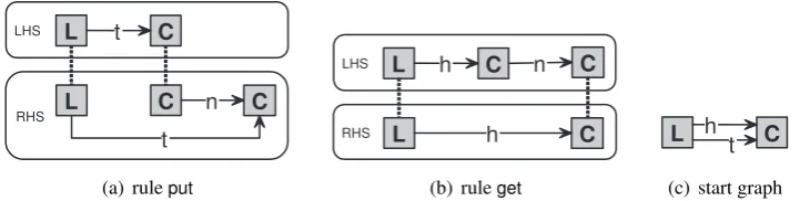
As an example throughout the paper we use a graph transformation system that models a single-linked list. The list is formed bycells, representing the elements in the list, which are connected by anextpointer. Additionally, a list has a root object that indicates the first and last elements, by way of pointers calledheadandtail. We consider two list operations: one thatputsa new element to the tail of the list, and another thatgetsthe head element from the list. These operations are modelled in our graph transformation system by two rules, shown in Figures 1(a) and 1(b). Simple abbreviations are used for conciseness. The corresponding morphisms between LHS and RHS of the rules are identified by dotted lines. Figure1(c)shows the start graph. For simplicity, we assume that our lists always have at least one element2.
It is clear that the concrete state space of the grammar in Figure 1is infinite: theputrule is always enabled, and successive applications of this rule keep producing longer and longer lists.
2.3 Neighbourhood abstraction
We work with directed edge-labelled graphs, where the labels are taken from a finite setLab. Formally, a graph is a tupleG=hN,Eiof nodes and edges, where the edges are tripleshv,a,wi
1More information about
GROOVEcan be found at the project website:http://groove.cs.utwente.nl.
LHS
RHS
L t C
L C n C
t
(a) ruleput
LHS
RHS
L h C
L C
C
h n
(b) ruleget
L h C
t
(c) start graph
Figure 1: A graph transformation system modelling a single-linked list.
L C n C
t
C
h n
n
Figure 2: A shape representing lists with four or more elements.
of source node, label, and target node; such thatv,w∈Nanda∈Lab. Node labels are simulated with self-edges; in fact we assume thatLabis partitioned into two sub-sets: unary (node) labels, and binary (edge) labels.
Our notion of abstraction is based on neighbourhood similarity: two nodes are considered indistinguishable if they have the same incoming and outgoing edges, and the opposite ends of those edges are also comparable. Graphs are abstracted by folding all indistinguishable nodes into one, while keeping count of their original number up to some bound of precision. The incident edges are also combined.
Counting up to some bound is done usingmultiplicities. We useMk={0, . . . ,k,ω}withk∈N
consisting of exact numbers up tok(which is typically a low value such as 1 or 2) and the value
ω standing for “many”.
The abstractions are calledshapes. They are 5-tuplesS=hG,∼,multn,multo,multiiin which • Gis the underlying graph structure of the shape;
• ∼ ⊆N×Nis aneighbourhood similarityrelation;
• multn:N→Mν is anode multiplicityfunction, which records how many concrete nodes were folded into a given abstract node, up to boundν;
• multo,multi: (N×Lab×N/∼)→Mµ are outgoing and incomingedge multiplicity func-tions, which record how many concrete edges with a certain label were folded into an abstract edge, up to a boundµ and a group of∼-similar opposite nodes.
Nodes and edges of a shape with multiplicity one are calledconcrete, otherwise they are called
collectors.
Figure2 shows an example of a shape. The graph structure of the shape is drawn as usual. The equivalence relation∼is indicated with dashed boxes. Node multiplicities are represented by line thickness: fat nodes have multiplicity ω, thin nodes have multiplicity one. All edge
3
Implementation
In this section we discuss the most important aspects of implementing the neighbourhood ab-straction theory inGROOVE.
The following is pseudo-code for generating the abstract state space.Qis the set of all shapes andFthe set of fresh, yet to be explored shapes;Pis the set of rules andGthe start graph. let S :=abstracti(G), Q := /0, F :={S}
while F6=/0
do choose S∈F (whichSis selected depends on the exploration strategy)
let F :=F\ {S}
for p∈P, m∈prematch(p,S), S0∈materialise(m,S)
do let R:=normalise(apply(p,m,S0))
if R∈/Q
then let Q :=Q∪ {R}, F :=F∪ {R}
fi od od
The important phases in this algorithm are
• abstractcomputes the shape of a graph. This is controlled by a parameteriexpressing the
radiusof the neighbourhood to be considered in the neighbourhood similarity relation. • prematchcomputes non-injective morphisms of a rulepinto a shapeS. Such a morphism
is not yet a match, because the images of p’s LHS may be elements with multiplicity greater than one; in this case they have to be materialised.
• materialise creates concrete nodes and edges for the image of p in S. This is a non-deterministic step, as there may be options involved in choosing multiplicities for the in-stantiated nodes and edges.
• applyis rule application, which can be carried out as usual because the rule now acts upon a concrete subgraph ofS0. At this step, the match of the rule is injective.
• normalisemerges the transformed graph back into the rest of the shape; it is thus similar toabstractexcept that it acts upon a (partially materialised) shape rather than a graph.
The following subsections present each of these phases in more detail.
3.1 Operationabstract
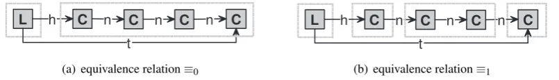
The abstraction uses the concept of neighbourhood equivalence over elements of a graph, de-noted≡i. It relates nodes with similar neighbourhoods, up to some positive “radius”i, which is a parameter of the abstraction. For a giveni>0 and graphG, operationabstractcomputes the relation≡ioverNGrecursively. For anyv,w∈NG, we have that
• v≡0w, ifvandwhave the same node labels;
• v≡iw, ifv≡i−1w, andvandwhave the same number of outgoing and incoming edges
for every edge label.
L C C
t
C
h n n C n
(a) equivalence relation≡0
L C C
t
C
h n n C n
(b) equivalence relation≡1
Figure 3: Iterations on the neighbourhood equivalence relation over a graph representing a list with four elements.
• NS=NG/≡i, i.e., nodes of the shape are the equivalence classes of≡i;
• ∼ =≡i−1, i.e., the shape equivalence relation is taken from the previous iteration of the
neighbourhood equivalence;
• multnis the multiplicity of each equivalence class in≡i, bounded byν;
• multo andmultiare the multiplicities of the set of edges between each node and equiva-lence class, bounded byµ.
An application of theabstract operation for our running example is shown in Figure3. We assume as input a graph representing a list of four elements, and also that the abstraction radius
i=1. Iteration≡0distinguish nodes based only on their labels, as can be seen in Figure3(a). Subsequent iterations refine the equivalence classes by looking at incoming and outgoing edges. This is shown in Figure3(b), where the first and last cells of the list are distinguished by the head and tail edges. The resulting shape built by operationabstractin this example corresponds to the one depicted in Figure2.
3.2 Operationsprematch,applyandnormalise
A pre-match m of the LHS of a rule p=hL,Ri into a shape S, is a non-injective morphism
m:L→GS, such that node and edge multiplicities are satisfied by the mapping. Operation
prematchuses the normal rule matching implemented inGROOVEand then removes the invalid matches by checking the conditions on multiplicities.
A pre-matchmhas to be massaged into aconcretematchm0, such that: (i)m0is injective; (ii) all nodes in the image ofm0are concrete and belong to a singleton equivalence class; and (iii) all edges in the image ofm0are concrete. This adjustment from pre-matchmto concrete matchm0
is done by thematerialiseoperation, explained in the next section.
Given a concrete matchm0into a materialised shapeS0, rule application is performed as usual. Operationapplysimply uses the normal transformation code fromGROOVE.
After transformation, a shape needs to be normalised, i.e., the concrete parts need to be merged back into the shape. This entails the computation of the≡i relation on shapes, which is similar to the one described in operationabstract.
3.3 Operationmaterialise
Op. Prio. Parameters Creates
matNode 0
nc∈S collector node, from which the new nodes will be materialised
Np⊆NL set of rule nodes mapped tonc by the pre-match
singNode
matEdge 1
ec∈S collector edge, from which the new edges will be materialised
Ep⊆EL set of rule edges mapped toecby the pre-match
pullNode
pullNode 2
e∈S edge that is pulling a new node fromnc
nc∈S collector node that is being pulled bye
u∈Mν multiplicity for the new node that will be created –
singNode 3 ns∈S the node to be singularised –
Table 1: Summary of the sub-operations of the materialisation phase. All operations are per-formed on a given shapeS, guided by the pre-match of the LHSLof a rulep.
Given a pre-match mof a rule p=hL,Riinto shape S, materialisefinds all shapes S0 such that f :S0 →S is a shape morphism and m0 :L→S0 is a concrete match. The challenge in implementing this step lies in transforming the descriptive solution just given into a constructive algorithm that produces the set of all possible materialisations, based on the given shapeSand pre-matchm.
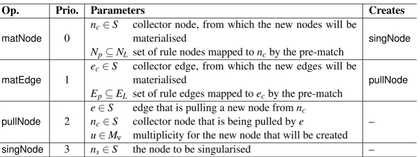
The materialisation algorithm iteratively changes the original shape in order to search for valid sub-shapes. The changes to be performed are divided into fourmaterialisation operations. A summary of these operations is given in Table 1. The second column of Table 1 lists the operation priority, with zero being the highest priority. All materialisation operations are non-deterministic. This implies that each operation may produce zero or more new materialisation objects. If the execution of the operation yields zero results, then it is said that the operation failed, i.e., performing the operation on the materialisation object does not produce a valid shape. Materialisation operations are put into a priority queue and traversed in a breadth-like fashion. When a materialisation is completed, it is moved to the result set ofmaterialise. Not all opera-tions can be determined when the materialisation process starts, so the execution of an operation can create other ones. The relation between creation of operations is given by the fourth column of Table1.
The main reason for splitting the materialisation phase in sub-operations is understandability. The rationale for splitting operations is that each materialisation operation must introduce only one level of non-determinism. We proceed to explain each operation of Table1in detail.
3.3.1 Equation systems
An equation system is a device used for searching valid shape configurations during the material-isation phase. OperationsmatEdgeandsingNodeuse equation systems. We present the common points here and discuss the particularities in the sub-sections describing the operations.
• set constraints, in the formx∈U, whereU is a set of arbitrary multiplicities. Variables occurring in this part of the system are calledconstrained.
• equations, in the formy=u−x, whereuis a constant multiplicity andxis a constrained variable. Variables occurring in the left-hand side of equations are calledderivedbecause their sets of values are obtained when the values of the constrained variables are fixed. • admissibility constraints, which restrict the overall admissibility of a shape configuration.
Such constraints are of the form∑t∈Ot≈∑t∈It, whereOandI are sets of outgoing and incoming terms, respectively. Atermis of the formu·x, whereuis a constant multiplicity value andxis a multiplicity variable. An admissibility constraint is satisfied if the resulting multiplicities produced by both sums are overlapping, i.e., have a non-empty intersection.
It is important to note that usual arithmetic symbols (e.g.,+and−) occurring in an equation system actually stand for operations on multiplicities. In particular, an equationy=u−xmay admit multiple solutions for a fixedx, namely the multiplicity values that when summed withx
equalu. More formally, given a valueux∈U for the constrained variablex, the possible values of the derived variableyare given byy∈ {uy∈Mk|ux+uy=u}, for a certain boundk.
Overlapping of multiplicities in the admissibility constraints is defined in terms of the intersec-tion of multiplicity intervals. The intuiintersec-tion goes as follows. Two multiplicities are overlapping if: (i) their values are equal, e.g., 1≈1, 16≈0, andω≈ω; or (ii) one multiplicity isω and the
other is a concrete value greater than the multiplicity bound, e.g.,ω≈2, and 16≈ω (assuming
multiplicity boundk=1).
Solving an equation system is done with a simple search algorithm that goes over all possible values for the constrained variables; calculates the values for the derived variables using the equations; and checks if all admissibility constraints are satisfied. Each valid solution produces a corresponding shape, obtained from the values of the variables.
3.3.2 Materialise Node
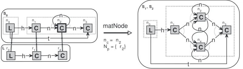
This operation materialises (creates) one or more nodes from a collector node nc, i.e., a node with multiplicity greater than one. As shown in the third column of Table1, the other parameter ofmatNodeisNp, the sub-set of nodes in the LHS of the rule that were mapped toncby the pre-match. The number of new copies of the collector node is determined by the cardinality of setNp. All new materialised nodes are created with multiplicity one and the mapping of the pre-match is adjusted to the new nodes. In addition, all edges adjacent toncare duplicated on the new nodes. The non-determinism of this operation comes from the choice on the remaining multiplicity of
nc, once the new nodes are materialised. This operation creates asingNodeoperation for each of the newly materialised nodes.
Figure4shows an example execution ofmatNode. On the left side of Figure4we see shape
S0 with a pre-match of the LHSLof ruleget. Since the image of rule noder2 is the collector noden2, it is necessary to materialise a concrete copy of n2. This leads to the application of
matNodewith parametersnc =n2 andNp={r2}. The operation creates a new concrete node n4 and duplicates all adjacent edges of n2, as can be seen on the right side of Figure4. The matNodeoperation in this example produces two new shapes, S1 andS2, which differ only in
S
0 n
L
L C n C
t
C
h n
L h C n C
r0 r1 r2
n0 n1 n2 n3
matNode
nc = n2 N
p = { r2} S
1, S2 n
L
C
C
n
t
C
h
n
C
n
n n
n
n0 n1 n3
n2
n4
Figure 4: Example of an execution of thematNodeoperation. ShapesS1andS2 differ only on the multiplicity of noden2:multnS1(n2) =1,mult
n
S2(n2) =ω.
thus,n2(which has multiplicityω) originally represents two or more nodes. When materialising
n4fromn2, the remaining multiplicity ofn2can be either one orω. Noden4will later be made
singular by asingNodeoperation.
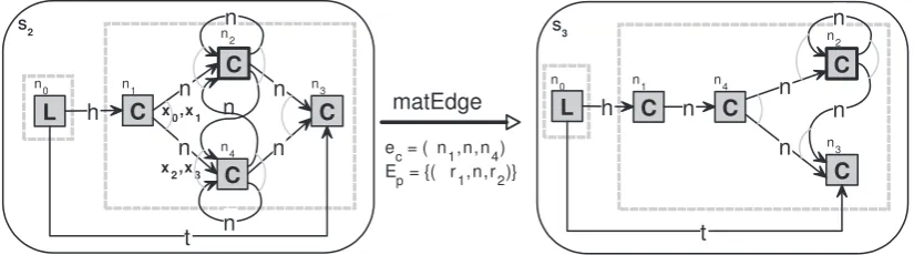
3.3.3 Materialise Edge
In the same vein ofmatNode, operationmatEdgematerialises (creates) one or more edges from a collector edgeec, i.e., an edge with outgoing or incoming multiplicities greater than one, or an edge that is part of an edge multiplicity bundle (shared edge multiplicity). The additional parameter of matEdgeisEp, the sub-set of edges in the LHS of the rule that were mapped to
ec by the pre-match (see Table 1). Similarly, the number of new copies of the collector edge is determined by the cardinality of setEp. The non-determinism of this operation comes from the choice on the remaining incoming and outgoing multiplicities ofec, once the new edges are materialised. This operation may create newpullNodeoperations.
Performing this operation involves constructing and solving an equation system. We create a pair of multiplicity variables for each edge bundle that is affected by the operation. One of the variables of the pair is taken as a constrained variable and the other as a derived one. In this equation system the set constraints are always formed by singletons sets3, with the value taken from |Ep|, i.e., the constrained variables stand for the number of concrete edges that will be extracted from the collector edge. The derived variables in the equations represent the remainder multiplicities of the collector edge or edge bundles. The admissibility constraints ensure that no invalid values are assigned to the derived variables, e.g., it is not possible to assign a multiplicity zero to an edge bundle that has one or more edges.
Figure5gives an example of application formatEdge. The input shape isS2, one of the results
of the matNodeoperation in Figure 4. AftermatNode materialises n4 and adjusts the match,
we see that the image of rule edge hr1,n,r2i is an edge with shared outgoing and incoming
multiplicities. This leads to the execution of the matEdge operation. In this execution, the
3This of course implies that the values for the constrained variables are already known. The reason for creating the
matEdge
ec = ( n1,n,n4) E
p = {( r1,n,r2)} S
2
x2,x3 x
0,x1
n
L
C
C
n
t
C
h
n
C
n
n n
n
n0 n1 n3
n2
n4
S
3 n
C
C
n1
n3 n2
n4
L
C
t
C
n0
h n n
n n
Figure 5: Example of an execution of thematEdgeoperation. This operation creates an equation system. The association of the equation system variables with edge multiplicities is shown in shapeS2. Variablesx0andx2are constrained, and variablesx1andx3are derived. This particular
execution ofmatEdgeis deterministic.
operation creates the following equation system
set constraints x0,x2∈ {1}
equations x1=1−x0 x3=1−x2
admissibility constraints x1+ω≈x3+ω
where the association of the multiplicity variables with edge bundles is shown in shapeS2 of
Figure5. The solution of this equation system is trivial, withx0=x2=1 andx1=x3=0. The
resulting shapeS3 is depicted on the right side of Figure 5. It is important to note that in this
particular example, the operation produces only one result shape. However, in the general case, matEdgereturns a set of results.
3.3.4 Pull Node
The theory of neighbourhood abstraction requires that all elements up to radiusiin the image of the match have to be concrete. After performingmatNodeandmatEdgeoperations, we obtain a rule match on which the elements of the image are concrete, but it is still possible to have abstract elements in the neighbourhood of the image. OperationpullNodetransforms the neighbourhood, by further materialising nodes when needed.
This operation is very similar tomatNode, with the exception that only one new node is cre-ated, which can have an arbitrary positive multiplicity, defined by parameteru. Note that, as in operationmatNode, all adjacent edges of the collector node are duplicated. The source of non-determinism ofpullNodeis the same as inmatNode, i.e., the choices on the remaining multiplicity of the collector node. The newly created node will not be singularised later; this operation does not create any new operations.
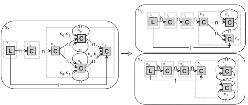
3.3.5 Singularise Node
S 6 C C n 1 n 3 n 2 n 4 L C C n 0 C n n n n n h n t n 5 S 5
x0,x1
n L C C n t C h n C n n n n n
0 n4 n3
n 2 n 5 C n 1 n
x4,x5
x2,x3
S 7 C C n 1 n 5 n 2 n 4 L C C n 0 C n n h n t n 3 n n
Figure 6: Example of an execution of the singNode operation with parameter ns=n4. This
operation also creates an equation system. The association of the equation system variables with edge multiplicity bundles is shown in shape S5. Variables x0, x2 andx4 are constrained, and
variablesx1,x3andx5are derived.
shape will no longer change. What is left to decide are the outgoing and incoming multiplicities of the edge bundles that will be affected by the operation.
In order to put a nodens in a singleton equivalence class,singNodecreates another equation system, where the variables represent the multiplicities of affected edge bundles. For each such bundles, we create a pair of variables. One variable of the pair, x, represents the multiplicity associated with the singular equivalence class that will be created; the other variable,y, stands for the multiplicity related to the remainder equivalence class after the split. Variablexis put in a set constraint, ranging on the set{0,1}, and variableygoes in an equation, i.e.,xis a constrained variable and y is a derived one. The admissibility constraints care for the sanity of the shape configuration after the split, such that valid solutions of the system produce valid final shapes.
Figure6shows asingNodeapplication with parameterns=n4. The input shapeS5is an
inter-mediate candidate shape produced during the materialisation. ThissingNodeexecution creates the following equation system
set constraints x0,x2,x4∈ {0,1}
equations x1=1−x0 x3=1−x2 x5=1−x4
admissibility constraints 1≈ω·x0+x2+x4 ω≈ω·x1+x3+x5
where the association of the multiplicity variables with edge bundles is shown in shapeS5 of
Figure6. This equation system has two solutions, namely: (i)x0=x2=x5=0 andx1=x3=
get put get put
put get put get
get
s
7
L th C C
n
s
6
L th C C
n
s
5
L C C
t
C
h n
n
s
4
L C C
t
C
h n
n
s
2
L C n C
t
C
h n
s0
L C
th
s1
L C
t
C
h n
put
s3
L C n C
t
C
h n
n
get put get put
get put
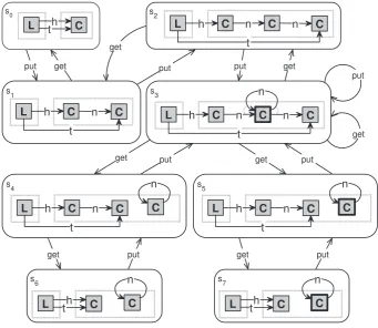
Figure 7: The abstract LTS of our running example, for the parametersi=1 andν=µ=1.
4
Results
When applying the implemented abstraction to our running example, we obtain the abstract state space depicted in Figure7. For an abstraction radius of one, the LTS has 8 states and 16 transitions. Each rounded box represents a state, with its numbering on the upper left corner, and the corresponding shape. The transitions between states are shown by arrows, labelled with the rule applied.
There are many interesting points to note in the state space of Figure7. First, as long as node and edge multiplicities stay within their bounds, the abstract graph transformation corresponds to the concrete one. This is seen on statess0,s1, ands2, where the shapes are concrete.
Second, an abstract state may represent an unbounded number of concrete ones. States3, for example, is an abstract representative for lists with four or more elements. This is illustrated by theputandgettransitions froms3to itself.
Third, the non-determinism of the materialisation algorithm can be seen from the four get transitions from states3. Although there is only one pre-matching of the rule, when materialising this pre-match several distinct shapes are produced.
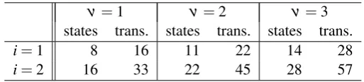
ν=1 ν=2 ν=3
states trans. states trans. states trans.
i=1 8 16 11 22 14 28
i=2 16 33 22 45 28 57
Table 2: State space sizes for a small variation of abstraction parameters (µ=1).
space. This spurious shapes arise from the fact that the neighbourhood abstraction mechanism does not keep information regarding connectivity. This is a point where we plan to improve the current theory.
After the abstract LTS is generated we can proceed to model check the properties of interest. For the LTS in Figure7, we can check, for example, that the following properties hold: (i) the head cell has no predecessors; (ii) the cells are not shared; and (iii) rulegetis applied infinitely often. Properties (i) and (ii) talk about safety and (iii) is a liveness property. They are informally described in English but can be easily translated into temporal logic formulae. Since these prop-erties hold in the abstract LTS, we can then conclude that they also hold in the infinite concrete state space.
5
Conclusions and future work
The results reported above are the very first steps toward the capability forGROOVEto incorpo-rate abstraction. We look upon this as a key factor in the eventual success of the tool. Though currently we have merely implemented the theory described in [BBKR08], we know from expe-rience that having the ability to actually experiment with smaller and larger cases provides a lot of additional motivation and can be a source of new ideas and developments.
For instance, only a working implementation makes it possible to obtain figures about actual abstract state space sizes, which is an important factor in the feasibility of any abstraction-based methods. Some very first figures about the effect of increasing node multiplicity boundsν and radiiiare collected in Table 2; the edge multiplicity bound µ was kept equal to one. Clearly,
the radius has greater effect on the state space size than the node multiplicity. All tests took just a few seconds to run. As an additional example we looked at the circular buffer grammar presented in [RD06]. In that paper the abstract state space was generated by hand, now we can mechanically reproduce it with the tool.
Bibliography
[BBKR08] J. Bauer, I. B. Boneva, M. E. Kurban, A. Rensink. A Modal-Logic Based Graph Abstraction. Pp. 321–335 in [EHRT08].
[BKK03] P. Baldan, B. K¨onig, B. K¨onig. A Logic for Analyzing Abstractions of Graph Transforma-tion Systems. In Cousot (ed.),Static Analysis Symposium (SAS). LNCS 2694, pp. 255–272.
Springer, 2003.
[CC77] P. Cousot, R. Cousot. Abstract Interpretation: A Unified Lattice Model for Static Analysis of
Programs by Construction or Approximation of Fixpoints. InPOPL. Pp. 238–252. 1977.
[EHRT08] H. Ehrig, R. Heckel, G. Rozenberg, G. Taentzer (eds.).International Conference on Graph
Transformations (ICGT). LNCS 5214. Springer, 2008.
[KK06] B. K¨onig, V. Kozioura. Counterexample-Guided Abstraction Refinement for the Analysis of
Graph Transformation Systems. InTACAS. LNCS 3920, pp. 197–211. Springer, 2006.
[KK08] B. K¨onig, V. Kozioura.AUGUR2— A New Version of a Tool for the Analysis of Graph
Trans-formation Systems.ENTCS211:201–210, 2008.
[RD06] A. Rensink, D. Distefano. Abstract Graph Transformation. In Mukhopadhyay et al. (eds.),
Software Verification and Validation. ENTCS 157, pp. 39–59. May 2006.
[Ren04] A. Rensink. Canonical Graph Shapes. In Schmidt (ed.),Programming Languages and
Sys-tems (ESOP). LNCS 2986, pp. 401–415. Springer, 2004.
[RN08] S. Rieger, T. Noll. Abstracting Complex Data Structures by Hyperedge Replacement. Pp. 69–
83 in [EHRT08].
[SRW98] S. Sagiv, T. W. Reps, R. Wilhelm. Solving Shape-Analysis Problems in Languages with
De-structive Updating.ACM ToPLaS20(1):1–50, 1998.
[SRW02] S. Sagiv, T. W. Reps, R. Wilhelm. Parametric shape analysis via 3-valued logic.ACM ToPLaS