Towards Hybrid LES-RANS-Coupling for Complex Flows with Separation

Eric Canc`es & Jean-Fr´ed´eric Gerbeau, Editors DOI: 10.1051/proc:2007010

TOWARDS HYBRID LES–RANS–COUPLING FOR COMPLEX FLOWS WITH

SEPARATION

Jaffr´

ezic B.

, Breuer M.

, Chikhaoui O.

, Deng G.

and Visonneau M.

Abstract. The paper is concerned with a new hybrid LES–RANS approach, which splits up the simulation into a near–wall RANS part and an outer LES part, both modes relying on a one–equation model for the turbulent kinetic energy. This model has been tested on the standard plane channel flow test case as well as on the flow over a periodic arrangement of hills. Encouraging results were achieved. In an additional study based on the detached–eddy simulation (DES) concept attempts have been made to improve the accuracy of the simulation by using adaptive local grid refinement. For this purpose, a criterion based on the residual of the budget of the mean momentum equations has been studied.

Introduction

Large–eddy simulation (LES) is a highly promising technique for the prediction of complex turbulent flows including large–scale flow phenomena such as massive separation, large recirculation regions and vortex shedding [6]. However, LES still suffers from the matter of fact that most turbulent flows of practical relevance cannot be computed because of the extremely large resources required, especially for high Reynolds number flows encountered in technical applications. In order to go beyond the present state–of–the–art, extremely fine grids required for the resolution of the near–wall region (e.g., thin boundary layers) have to be avoided.

For this purpose a hybrid LES–RANS approach is developed, which tries to split up the simulation (ideally not the domain) into a RANS part and an LES part. Typically, RANS is adequate for attached boundary layers requiring reasonable CPU–time and memory, where LES can also be applied but demands extremely large resources. Contrarily, RANS often fails in flows with massive separation and/or with large–scale vortical structures. Here, LES is without doubt the best choice. The basic concept is to combine the advantages of both methods yielding an optimal solution at least for a special class of flows. A real non–zonal hybrid technique is preferred since it avoids the predefinition of RANS and LES regions leading to an approach where the suitable simulation technique is chosen more or less automatically. This is a big advantage compared to Detached–Eddy Simulation (DES) formulated by Spalart [27]. Although DES is claimed to be a non–zonal approach by the authors, a close look at the switching criterion shows that the interface location is closely related to the grid design and thus predefined by the user. The hybrid strategy proposed in this paper avoids this grid dependency

∗_{The project is financially supported by the Deutsche Forschungsgemeinschaft (BR 1847/8–1) and the Centre National de la}

Recherche Scientifique within the French–German Programme ’LES for complex flows’ (FOR 507). The computations were partially carried out at RRZE Erlangen, LRZ M¨unchen, IDRIS and CINES. The organization of CEMRACS 2005 and all kinds of support are gratefully acknowledged.

1_{Institute of Fluid Mechanics, University of Erlangen–N¨urnberg, Cauerstr. 4, D–91058 Erlangen, Germany;}

e-mail: [email protected] & [email protected]

2_{Ecole Centrale de Nantes, Laboratoire de M´ecanique des Fluides CNRS UMR 6598, Nantes, France;}

e-mail: [email protected] & [email protected] & [email protected]

c

EDP Sciences, SMAI 2007

by defining the interface based on physical issues (see Section 1.3). Although the idea of combined LES–RANS methods is not new, a variety of open questions has to be answered. This includes in particular the demand for appropriate coupling techniques between LES and RANS, adaptive control mechanisms, and proper SGS/RANS models.

Additionally, a study has been carried out on a local grid refinement approach. Indeed, in LES systematic refinement is usually adopted to solve the problem of insufficient spatial resolution leading to extremely fine grids, especially in the very expensive near–wall region. Thus a choice for a local grid refinement criterion based on mean quantities provided directly by the simulations is proposed. This approach is assumed to be an interesting issue for improvements of the spatial resolution without excessive resource requirements.

In order to investigate the above mentioned open questions, the ’flow over periodic hills’ test case including pressure–induced flow separation and subsequent reattachment is considered in addition to the standard plane channel flow test case.

1.

Hybrid LES–RANS method

A variety of different hybrid concepts were proposed in the literature. A crude distinction between various proposals is given byzonal andnon–zonaltechniques. In the first case, the user predefines the LES and RANS regions, which is often difficult to carry out for unknown flows. Conversely, the non–zonal approach chooses (more or less) automatically the suitable simulation technique and thus avoids the region predefinition. Here a gradual transition between both methods takes place which weakens the problem of setting up an appropriate coupling strategy between RANS and LES zones not available today. Hence in the present study a non–zonal approach is preferred. Another important issue is the question of suitable models for such hybrid methods. For the non–zonal methodology a unique model is more advantageous. In the context of eddy–viscosity models for RANS, a two–equation model is a natural choice since one transport equation is solved for the velocity scale and one for the length scale. For LES zero– or one–equation models are more obvious since the length scale is naturally given by the filter width Δ. Consequently, these facts are in contradiction to a unique model. However, if the near–wall region is the main target for RANS, the length scale can be prescribed by an algebraic relation. This leads to a one–equation model for both zones.

For the near–wall RANS region the model adopted in the present study is based on the two–layer approach proposed by Rodi et al. [23]. They used a one–equation model for the viscosity–affected near–wall layer and combined it with a standardk–model for the outer region to a two–layer RANS model. Hence, the formulation for the inner layer is taken over, but the outer region is basically replaced by LES. The resulting unique model consists of a transport equation for the modeled turbulent kinetic energy kmod in the RANS mode and the subgrid scale (SGS) turbulent kinetic energyksgs in the LES mode, respectively. The two models are then distinguished by their definitions of the dissipation rateof the turbulent kinetic energy and the eddy–viscosity

νt(see Sections 1.1 and 1.2).

The general transport equation forkreads:

∂k

∂t +Uj ∂k

∂xj

= ∂

∂xj

(ν+ νt

σk )∂k

∂xj

+νt

∂Ui

∂xj +∂Uj

∂xi

∂Ui

∂xj −

(1)

with σk = 1.0

Ui has to be understood as time–averagedUi in RANS mode and filteredUiin LES mode.

1.1.

SGS model for the hybrid technique

The standard formulation ofandνtfor the SGS one–equation model [21, 24, 25, 29] reads:

νt = Cμk1sgs/2Δ (2)

= Cdk3sgs/2/Δ (3)

Δ = (ΔxΔy Δz)1/3 (4)

Thus the decision had to be taken on the value of the constantsCd and Cμ used for the definition of and

νt, respectively. For this purpose several sets of constants have been tested on the plane channel flow test case. The tests were performed applying constants suggested by Schumann [25], Yoshizawa [29] and Pope [21] relying on the Kolmogorov energy spectrum as well as a model proposed by Sagaut [24] also based on the energy spectrum but using spectral methods such as EDQNM (Eddy–Damped Quasi–Normal Markovian) the-ory for the adjustment of the constants. All models gave similar results. Therefore, it has been decided that the main set should be Cμ = 0.05 andCd = 1.0 as proposed by Schumann. However, as will be seen in Sec-tion 5.2 the LES models have to be checked for more complex flow situaSec-tions and under varying grid resoluSec-tions.

1.2.

RANS model for the hybrid technique

The next step of the study was to define the RANS model which is applied in the hybrid LES–RANS technique. The objective was to use a simple model based on the turbulent kinetic energy and due to the restricted area in which the model operates, especially designed for the near–wall region. Moreover, it is preferred to avoid the disadvantage of using damping functions, which are normally required for the length scalelμand the dissipation lengthl. One model meets these mentioned key points.

In order to improve the quality of the prediction of the RANS technique, Rodi et al. [23] formulated a one– equation near–wall turbulence model. The particularity of the model is the use of the wall–normal velocity fluctuationsv2 as the velocity scale instead ofk. As a consequence only one damping function is required. The formulation shown below is the original model suggested by Rodi et al. [23], which was combined with thek– model in the outer region to a two–layer RANS approach.

The empirical relations forνtandv2read:

νt = (v2)1/2lμ,v (5)

lμ,v = Cl,μy (6)

v2_{/kmod = 4.65×10}−5_y∗2_{+ 4.00×10}−4_y∗ _{for y}∗_{≤60 (7)}

y∗ _{= k}1/₂

mody/ν (8)

Cl,μ = 0.33 (9)

The empirical relations forare given by:

= (v2)1/2kmod/l,v (10)

l,v = 1.3y/

1 + 2.12 ν (v2)1/_2y

(11)

As shown by Rodi et al. [23] and originally introduced by Durbin [14], for the near–wall region (RANS mode) the wall–normal velocity fluctuations (v2)1/_{2are better suited to characterize the turbulent motion than using}

lengthl,v used to define the dissipation rate, which usually reads =Cd k3/2/l in a one–equation model, also scales linearly near the wall. Only in the immediate vicinity of the wall the distribution must be modified to yield the correct behavior of∼y0 as y goes to zero. In order to apply (v2)1/2 _{as the velocity scale in the} model, Rodi et al. provided an equation to relate the wall–normal velocity fluctuations to the distribution of

k(equivalent tokmodin RANS mode) so that the transport equation does not have to be adjusted. Instead of usingy+, formulated with uτ, they introducedy∗, which allows the model to be applied in separated flows, for whichτw is zero or negative. This formulation ofv2is valid up toy∗≈60, which according to DNS results [18] corresponds to y+ ≈ 30. Finally, one can notice that the constant Cμ usually used in the eddy–viscosity definition is now included in the eddy–viscosity length scale relation.

1.3.

LES–RANS interface

Two critical points are how to combine both techniques and how to choose a criterion to shift from RANS to LES. In Rodi et al.’s two–layer approach [23], the ratio of the eddy–viscosity to the molecular viscosityνt/ν is employed as switching criterion. In the vicinity of the wall, the one–equation near–wall turbulence model is applied until the ratio reaches a fixed valueCswitch. Then the outer model is used. In order to keep the requirementy∗≤60, Cswitch was set to 16 by Rodi et al. [23]. In the hybrid LES–RANS technique this value cannot be applied asνt in the LES mode is much lower than νt in the RANS mode. Furthermore, once the critical value ofνt ((νt)crit =ν·Cswitch) is attained in the RANS mode,νt will strongly decrease in the LES mode and hence fall below the critical value (νt)critagain. Then the entire simulation is treated in RANS what is not desired. The suitable ratio for the LES–RANS switch is found forCswitch<1. However, this criterion did not offer suitable results. Although the simulation shifts from RANS to LES at a reasonable distance from the wall, the technique switches back from LES to RANS in the core of the domain when νt decreases and finally reaches the critical ratio (νt)crit. Therefore, this criterion has been abandoned. As a remedy for the present hybrid LES–RANS technique, different dynamic switching criteria have been tested to define the interface between RANS and LES:

• Validity restriction of (v2):

y∗_{≤60 =C}

switch (12)

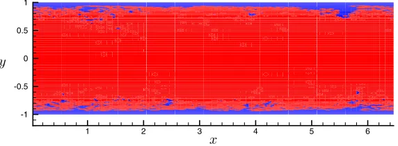
Here the dynamic criteriony∗based onkis applied to define the LES–RANS interface. This condition gives, in the channel flow test case, no real delimited LES–RANS regions (see Fig. 1 and the following criteriony∗₂ for explanation). The hybrid LES–RANS technique using the present criterion is named ’hybrid version A’.

1 2 3 4 5 6

-1 -0.5 0 0.5 1

y

x

Figure 1:Channel flow test case at Reτ = 590. RANS–LES domain layout. RANS domain: blue zone. LES domain:

0 1 1 2 3 4 5

10 100

y

k

k

k

0.1 0

1 1 2 3 4 5 6 7

10 100

y

k

k

k

k

0 1 1 2 3 4 5 6 7

10 100

y

k

k

k

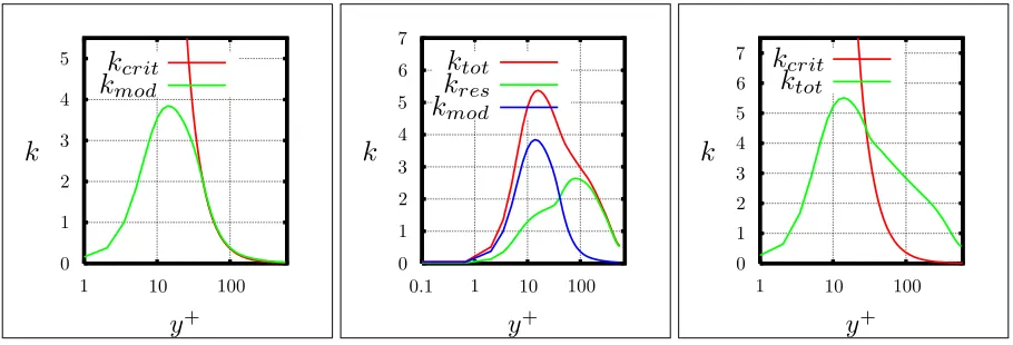
Figure 2:Results for the channel flow test case atReτ = 590. Behavior ofkmod in comparison withkcrit(left). kmod, kres and ktot of hybrid version A (center). Behavior ofktot used in y2∗ in comparison with kcrit in hybrid

version B (right).

• New criteriony∗₂:

y∗

2 ≤60 =Cswitch (13)

In order to get over the last remark, the new criteriony∗₂ is introduced, which is defined as follows

y∗

2 = ktot1/2y/ν. Hence y2∗ is a modification of y∗ by replacing kmod by ktot =kmod+kres. Here ktot and kres denote the total and the resolved turbulent kinetic energy, respectively. After testing y∗, it was seen that no clearly delimited RANS and LES regions were obtained. This fact is a consequence of kmod used in the formulation of y∗. As can be seen in Fig. 2 (left), kmod used in ’hybrid version A’ closely follows the curve kcrit, which is defined askcrit = (Cswitchν/y)2 and represents the limit between RANS and LES (kmod ≤kcrit meaning RANS mode). As a remedy the presence of resolved turbulent scales in the RANS region (see Fig. 2, center) is accounted for. Indeed, in steady RANSkmod is expected to correspond to ktot and thus kres should be zero. That is not the case here. Since it operates as an unsteady RANS (URANS), also the RANS mode resolves some turbulent scales. Thus

kmod in y∗ is replaced by ktot, which gives a higher value of k used in the switching criterion and by this way is assumed to provide two distinct RANS and LES domains. The effect of this modification is observed in Fig. 2 (right). Unlikey∗,y₂∗ provides a sharp interface between RANS and LES.

It has to be noticed that the condition y∗₂ ≤60 always keeps the requirement y∗ ≤60 and that y∗ is kept in the formulation of the model. The LES–RANS interface usingy₂∗≤60 as criterion is located at

y+_{≈30. The hybrid LES–RANS technique using the present criterion is named ’hybrid version B’.}

1.4.

Modified formulations of the RANS model

1.4.1. Adjustment of the RANS model to a higher Reynolds number.

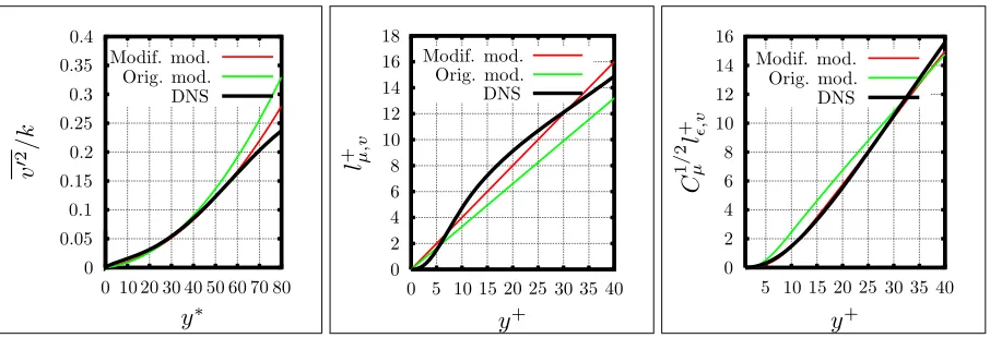
In order to match the objectives of the present study, i.e. to apply LES to high Reynolds number turbulent flows, the model performance has been compared with a more recent, higher Reynolds number (Reτ = 590) DNS of a channel flow (see Section 4.1) compared to the reference DNS used by Rodi (Reτ = 180 and 395). This study shows that an adjustment of the constants is worth being tested (see Fig. 3). An enhanced RANS model using the same architecture but modified constants leading to a much better agreement between the modeled and the real distributions ofv2/k,lμ,v+ andC1

/2

0 0

10 20 30 40 50 60 70 80 0.05 0.1 0.15 0.2 0.25 0.3 0.35 0.4

y

v

/k

5 1015 25 35

10

20 30 40

2 4 6 8 12 14 16 18

y

l

5 1015 25 35

10

20 30 40

2 4 6 8 12 14 16

y

C

l

Figure 3:Channel Flow: Distribution of v2/k (left), l_μ,v+ (center) andCμ1/2l+,v (right). Modif. model: New model formulation using DNS results of Moser et al. [18] atReτ= 590. Orig. model: Rodi et al.’s formulation [23] based on low–Re results but plotted for DNS results of Moser et al. [18] atReτ = 590.

The new empirical relations forνtandread:

v2_{/kmod = 3.55×10}−5_y∗2

2 + 6.50×10−4y2∗ for y2∗≤60 (14)

Cl,μ = 0.40 (15)

l,v = 1.5y /

1 + 7.65 ν (v2)1/2_y

(16)

This new set of constants can be applied to each previously described model versions (A and B), which are namedhybrid versions Am andBm when the new set of constants is employed.

1.4.2. Adjustment of the RANS eddy–viscosity.

This second modification is a consequence of the presence of resolved turbulent scales in the RANS region. Indeed, as previously mentioned (see Section 1.3) in steady RANS (uiuj)modcorresponds to (uiuj)tot and the modeled eddy–viscosityνmod

t,RANS provided by the model is the total eddy–viscosityνt,RANStot . Nevertheless, the first campaign of tests carried out on the hybrid approach (see Section 5.1.1) showed a different outcome with the pronounced presence of resolved turbulent scales in the RANS region. Under this conditionνt,RANStot cannot be longer seen asνmod

t,RANS but represents the sum ofνt,RANSmod and a resolved eddy–viscosityνt,RANSres . Thisνt,RANSres is obviously not explicitly calculated but depicts the effect of the resolved field.

According to this remark the important contribution of the resolved field might also be taken into account and the formulation of the RANS model, as part of the hybrid LES–RANS approach, be somehow adjusted. In the RANS model,νmod

t,RANS is calculated withkmod, which is notktot because of the unsteady character of the simulation and thus lower than a correspondingkmodcomputed in steady RANS. Therefore, the resolved field is already accounted for in the calculation ofνt,RANSmod . Nevertheless, the under–prediction ofU in the channel flow test case (see Fig. 4), which could be explained by the over–prediction ofνtot

t,RANS seems to show that this automatic adjustment of the model is insufficient. This statement is confirmed by Fig. 5 (left), which presents

νmod

t,RANS. In the RANS region the modeled νt closely followsνt provided by DNS results but representing the reference total eddy–viscosity νt,RANStot . Therefore, it can be assumed that ν

tot

t,RANS in the case of the hybrid LES–RANS technique is over–predicted.

0 5 10 15 20

1 10 100

y

U

Am Bm

DNS

0 1 2 3 4 5 6

1 10 100

y

k

kmod

ktot

kres

DNS

0 1 2 3 4 5 6

1 10 100

y

k

kmod

ktot

kres

DNS

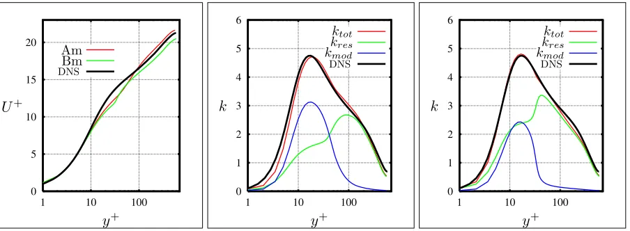
Figure 4:Results for the channel flow test case atReτ = 590. Predictions of the mean streamwise velocityU+ for the

cases hybrid versions Am andBm (left), k forhybrid versions Am (center) andBm (right). DNS result of Moser et al. [18].

byk. Additionally, the ratio (uv)res/(uv)tot versusy₂∗ (Fig. 5, right) obtained from the statistical results of the plane channel flow withhybrid version Bm never passes below 0.3 (value at the positiony₂∗= 12 ory+≈7) in the relevant RANS region and reaches 0.65 close to the interface (y∗₂ = 60 ory+≈30). This result exhibits the importance of this resolved field in the RANS region and the persistency of the resolved scales which do not vanish as expected. The significant level of the resolved field is plausibly due to the position of the interface relatively close to the wall as well as the high resolution of the grid used (see Section 5.1). The questions arising now are: shouldνmod

t,RANS be readjusted? If yes, should this adjustment be performed according to (uv)res? If yes, how should the resolved Reynolds shear stress field be ’introduced’ in the RANS formulation?

Assuming that the two first questions can be answered positively, the remaining one is how to adjust the eddy– viscosity. A natural choice to observe the importance of the resolved shear stress in the simulation is the ratio (uv)res/(uv)tot. A function providing this ratio could be an interesting starting point and the adjustment of

νmod

t,RANS could resemble to νt,RANSmod =νt,RANSmod ·(1−f) withf representing the effect of (uv)res.

In order to verify these assumptions, an empirical functionf(y₂∗) (with no character of generality) mimicing the ratio (uv)res/(uv)tot (see Fig. 5, right) is formulated:

⎧ ⎨ ⎩

f(y∗₂) = 0.3·y∗₂ for 0≤y∗₂≤1

f(y∗₂) = 0.3 for 1< y∗₂≤12

f(y∗₂) = 0.3 +1.55·10−4·(y₂∗−12)2 for 12< y∗₂≤60

νmod t,RANS =ν

mod,temp

t,RANS ·(1−f(y2∗)) (17)

This functionf(y∗₂) compensating for the presence of (uv)res in the formulation ofνt,RANSmod is used as follows.

νmod

t,RANS is first calculated as previously mentioned in hybrid version Bm providing ν

mod,temp

t,RANS . In a second step the function f(y∗₂) is applied, giving the effective νt,RANSmod . An important remark is that the function

0 2 4 6 8 10 1 10

y

ν

/ν

0.1 1 10 100

y

(

u

v

)

0 10 20 30 40 50 60

y

(

u

v

)

/

(

u

v

)

f(ratioy∗₂)

Figure 5:Results for the channel flow test case at Reτ = 590. νt,RANSmod /ν (left) and resolved Reynolds stresses uv (center) for thehybrid versions A, B, Am andBm. Ratio (uv)res/(uv)tot for thehybrid version Bm and function f(y₂∗) (right). LES–RANS interface aty₂∗= 60 (y+≈30) forversions B andBm.

function has provided equivalent improvements than the present empirical functionf(y₂∗) for which the results are shown in Section 5.1.3.

2.

Adaptive grid refinement

For LES and DES simulations it was found that the results are more sensitive to the grid quality and density compared with a RANS computation. Only a few articles in the literature deals with adaptive local grid refinement applied to these specific simulations. Generally, the solution used is a systematic refinement which increases considerably the required resources.

In order to improve the accuracy of LES and DES simulations, attempts to perform an adaptive grid refinement have been carried out in order to take benefit of the unstructured solver (see Section 3.2). The focus here has been to study the behavior of the residual of the budget for the mean momentum equations in DES to provide a criterion for local grid refinement. The grid and the results obtained using this criterion are presented for the case of the flow over the periodic hill in Section 5.4.

3.

Numerical Methodology

The present study involves two different groups and the computations are performed applying two different codes. The first, namelyLESOCC is used by LSTM Erlangen, whereas the simulations by Ecole Centrale de Nantes are performed with the ISIS code.

3.1.

LESOCC

3.2.

ISIS

To handle complex geometries efficiently, an unstructured code ISIS [10–12] is developed at Ecole Centrale de Nantes. It is a finite–volume code solving the Navier–Stokes equations for an incompressible fluid using arbitrary control volumes. The convective fluxes are discretized with a second–order central scheme or an upwind–blended scheme. A second–order central scheme is applied to the diffusion fluxes. A second–order backward differences implicit scheme is employed for time discretization. Pseudo–time stepping is used for steady flow computations. The Rhie and Chow approach [22] is employed to evaluate the mass flux in a non– staggered layout. The velocity–pressure coupling is solved by a SIMPLE like algorithm. The pressure equation is solved with a preconditioned conjugate gradient solver. The code was initially designed for RANS simulation. Several statistical models ranging from one–equation Spalart–Allmaras, two–equation linear and non–linear models such as k–ω SST model and explicit algebraic stress model, to seven–equation differential Reynolds stress model are implemented and extensively validated [10–12]. ISIS was also validated successfully in the context of DNS, LES and hybrid LES/RANS (mainly DES) upon different classical test cases [9].

4.

Test Cases

4.1.

Plane channel flow

The first test case used for validating the basic settings and model modifications, is a plane channel flow with periodic boundary conditions in streamwise and spanwise directions and no–slip boundary condition at the walls. The dimensions are: 2π (streamwise) ×π (spanwise) ×2 (wall–normal direction). The results of our tests are compared with DNS data of fully developed plane turbulent channel flow at a Reynolds number ofReτ = 590 (Reb= 10,935) provided by Moser et al. [18].

4.2.

Periodic hill flow

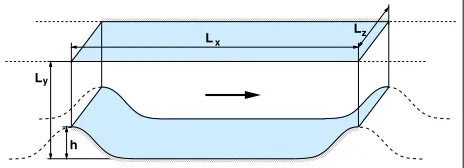
The hill flow configuration was a test case at the ’ERCOFTAC/IAHR/COST Workshop on Refined Turbu-lence Modeling’ in 2001 and 2002 [16,17]. The basic idea is to set up a geometrical ’simple’ test case which allows to perform basic investigations based on a ’complex’ flow including pressure–induced separation and subsequent reattachment. Fig. 6 shows a sketch of the configuration. The dimensions of the domain are: Lx(streamwise direction) 9.0h, Ly (wall–normal direction) 3.035hand Lz (spanwise direction) 4.5h. The flow is assumed to be periodic in the streamwise direction. As no DNS was performed at the Reynolds number ofReb= 10,595,

00000000000000000000000000000000000 00000000000000000000000000000000000 00000000000000000000000000000000000 00000000000000000000000000000000000 00000000000000000000000000000000000

11111111111111111111111111111111111 11111111111111111111111111111111111 11111111111111111111111111111111111 11111111111111111111111111111111111 11111111111111111111111111111111111

00000000000000000000000000000000000

11111111111111111111111111111111111

000000000000000000000000000000000000

111111111111111111111111111111111111

00000000000000000000000000000000000 00000000000000000000000000000000000 00000000000000000000000000000000000 00000000000000000000000000000000000 00000000000000000000000000000000000

11111111111111111111111111111111111 11111111111111111111111111111111111 11111111111111111111111111111111111 11111111111111111111111111111111111 11111111111111111111111111111111111

L_x Lz

y L

h

Figure 6: 3D sketch of the periodic hill flow test case.

wall shear stress were observed and the y+ value reaches its maximum of about 1.2. Hence the lower wall is well resolved. Regarding the wall–normal resolution the grid satisfies the requirements of a wall–resolved LES prediction. Compared to previous studies [15, 28] who employed in their highly resolved simulations a curvilinear grid with about 4.6 million CVs especially the number of grid points in the wall–normal direction was increased in our reference solution. Furthermore, the simulations resolve not only the lower wall (the hills) in more detail but also resolve the upper wall by a DNS–like representation (y+ ≤ 0.95). Thus in contrast to [15, 28] the application of a wall function is avoided. Overall the grid is much finer than in [15, 28]. For example, the cell sizes at the hill crest, which is a key region for the periodic hill flow are in the current case Δxcrest/h= 0.026 and Δycrest/h= 2.0·10−3whereas the corresponding values in [15,28] are Δxcrest/h= 0.032 and Δycrest/h= 3.3·10−3, respectively. Owing to the increased resolution in streamwise and spanwise direc-tions the cell sizes expressed in wall units are below Δx+= 20 and Δz+= 9 and thus lower than in [15, 28] and substantially lower than the recommendations for wall–resolved LES given by Piomelli and Chasnov [20]. That also holds at the windward slope of the hill where the largest shear stresses are found. In the reference simulation the dynamic eddy–viscosity model was applied. The boundary conditions were as follows: no–slip conditions at the walls and periodic boundary conditions in spanwise and streamwise directions (fixed mass flow rate). To gather reliable statistical data the flow was averaged in time (dimensionless averaging timeTavg= 1277.34) and along the homogeneous spanwise direction.

In the present investigation simulations for the hill configuration are performed on 4 different grids. Grid A

0 2 4 6 8

0 1 2 3

y

x

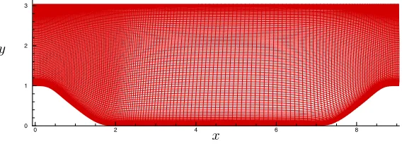
Figure 7: Periodic hill flow test case. Grid B.

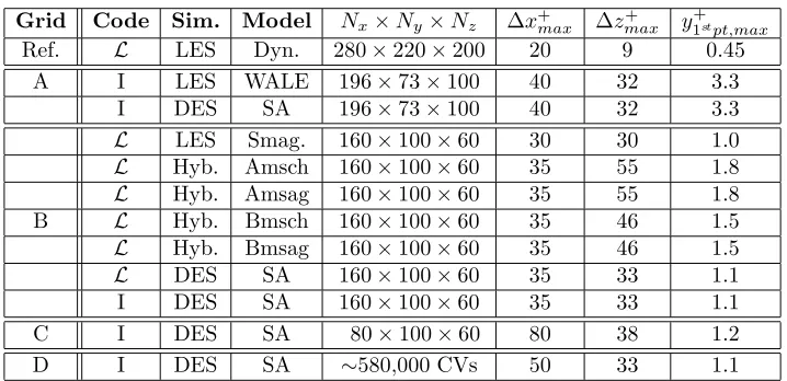
(196×73×100) is designed for coarse LES simulation. The height of the first grid cell on the crest of the hill is Δycrest/h = 0.01. Grid B (Fig. 7) consists of 160×100×60 control volumes in streamwise, wall–normal (res.: Δycrest/h = 0.005, 1st CV height) and spanwise directions, respectively. It has to be mentioned that grid B has been especially designed for DES. The number of grid points in the spanwise direction is reduced compared with grid A so that the RANS region becomes larger. In this configuration the DES technique using the Spalart–Allmaras model switches from RANS to LES at a distance of about 7–9 RANS cells instead of 4–5 RANS cells for grid A. To study the grid dependency of the DES simulations, a third grid has been used (grid C: 80×100×60), extracted from grid B by retaining every second grid point in the streamwise direction. The RANS region in the DES context for this grid covers 12–14 control volumes away from the wall. Finally, grid D has been designed by using the proposed adaptive grid refinement method applied on grid C (see Section 5.4). Table 1 summarizes the most important characteristics of all simulations carried out for the hill flow test case.

5.

Results

Grid Code Sim. Model Nx×Ny×Nz Δx+max Δzmax+ y₁+stpt,max

Ref. L LES Dyn. 280×220×200 20 9 0.45

A I LES WALE 196×73×100 40 32 3.3

I DES SA 196×73×100 40 32 3.3

L LES Smag. 160×100×60 30 30 1.0

L Hyb. Amsch 160×100×60 35 55 1.8

L Hyb. Amsag 160×100×60 35 55 1.8

B L Hyb. Bmsch 160×100×60 35 46 1.5

L Hyb. Bmsag 160×100×60 35 46 1.5

L DES SA 160×100×60 35 33 1.1

I DES SA 160×100×60 35 33 1.1

C I DES SA 80×100×60 80 38 1.2

D I DES SA ∼580,000 CVs 50 33 1.1

Table 1:Hill flow grid resolutions for each simulations. Abbreviations: Ref.: Reference. L: LESOCC. I: ISIS. Smag.:

Smagorinsky SGS model. Dyn.: Dynamic Smagorinsky SGS model. WALE: Wale SGS model. SA: Spalart– Allmaras model. Nx,Ny,Nz: Number of control volumes in streamwise, wall–normal and spanwise directions, respectively. Δx+

max, Δz+max andy₁+stpt,maxare given for the rangex/h= 0 to 8.0. At the windward side of the hill the resolution decreases owing to the increased value of uτ in this region.

5.1.

Hybrid LES–RANS technique: Channel flow

5.1.1. Versions A and B.

For the classical plane channel flow test case (Reb = 10,935) the new hybrid model provides encouraging statistical results for a coarse (64×64×64 control volumes) and a fine grid (128×128×128 control volumes). For these resolutions the first grid point (half first cell) is located at positiony+= 1.46 and y+= 0.68 for the coarse and fine grids, respectively. The results presented and discussed concern the fine grid only. The results on the coarse resolution can be found in [2].

The switching location of the LES–RANS interface is located at y+ ≈30 for hybrid version B, which is the position expected and estimated based on DNS results. As mentioned in Section 1.3,hybrid version Adoes not give a precise interface location.

Compared with the DNS data a higher uτ value is found in the case of the hybrid LES–RANS version B (deviation of +3.4%) whereashybrid version Apredicts a loweruτ value (deviation of−2.3%). The streamwise velocity of both hybrid versions shows discrepancies in comparison with the DNS reference (see Fig. 8) starting from the core of the RANS region. Furthermore,U presents an inflection point at the location of the interface (y+ ≈30). This behavior is also observed on theuures curve. This can be explained by the sudden drop of

νmod

0 5 10 15 20 25

1 10 100

y

U

0.1 1 10 100

y

rm

s

(

u

u

)

0.1 1 10 100

y

rm

s

(

v

v

)

0.1 1 10 100

y

(

u

v

)

0.1 1 10 100

y

k

A B DNS 0 1 2 3 4 5 6

0.1 1 10 100

y

k

A B DNS

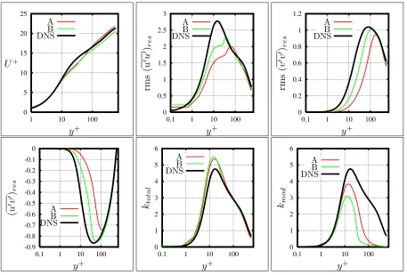
Figure 8:Result for the channel flow test case (Re=10,935) ofhybrid versions A and B. Mean streamwise velocityU+

(upper left). Resolved Reynolds stressesuu(upper center) andvv (upper right). Resolved Reynolds shear stress u_v (lower left). Turbulent kinetic energies ktot (lower center) andkmod (lower right). Values scaled withuτ of each case, respectively. DNS data provided by Moser et al. [18].

from RANS to LES at a clear position, however, it is clear that it offers a more extended RANS region. The consequence is the larger proportion given to the modeled scales inversion A.

5.1.2. Versions Am and Bm.

The first modification carried out on the near–wall model (see Section 1.4.1) only marginally modifies the resolved field as visible in Fig. 9 (center). However, the total turbulent kinetic energy given by the DNS is now predicted accurately by hybrid versions Am and Bm. Since the results of these two versions are similar, onlyhybrid versions B and Bm are compared in Fig. 9. Obviously, the adjustment of the RANS model leads to a reduction of the modeled turbulent kinetic energy. However, as previously mentioned, kres is kept nearly unchanged. The uτ value for the versions Am and Bm are unchanged compared to the versions A and B, respectively. The same remark is valid for the prediction of the mean streamwise velocity.

5.1.3. Versions Bmf with the compensating functionf(y₂∗).

0 1 2 3 4 5 6

0.1 1 10 100

y

k

B Bm DNS

0 1 2 3 4 5 6

0.1 1 10 100

y

k

s

B Bm DNS

0 1 2 3 4 5 6

0.1 1 10 100

y

k

B Bm DNS

Figure 9:Result for the channel flow test case (Re=10,935). Turbulent kinetic energies ktot (left), kres (center) and

kmod (right) forhybrid versions B andBm. LES–RANS interface aty+≈30. Values scaled byu2τ of each case, respectively. DNS data provided by Moser et al. [18].

is presently studied in order to propose a solution to resolve this discrepancy. In relation to the previous obser-vation forU+the prediction of the wall shear stress is in really good agreement with the DNS value (+0.26% for Bmf compared with +3.22% forBm). The resolved turbulent kinetic energy is increased in the RANS region which is not balanced by the reduction of the modeled part resulting in an over–predicted total kinetic energy

ktot.

The function f(y₂∗) is presently used to adjust νmod

t,RANS according to the proportion of (uv)res in the RANS region. This leads to a significant reduction of the νt,RANSmod value. The maximal instantaneous value of the ratioνmod

t,RANS/ν is 7.6, 2.7 and 1.007 for thehybrid versions Bm and Bmf and the LES using the one–equation SGS model with Schumann’s constants, respectively. As can be noticed the functionf(y₂∗) brings the hybrid LES–RANS method too close to an LES level, which is not desired. Nevertheless, this type of function will be tested with thehybrid version Am, which offers a lower level of resolved contributions and a higherνt,RANSmod value. Thus the resultinghybrid version Amf should provide a suitableνmod

t,RANS value.

5.2.

Hybrid LES–RANS technique: Periodic hill flow simulation

The second, reasonably complex test case is the flow over periodic hills (Reb = 10,595). To assess the new hybrid approach, grid B is used (depicted in Fig. 7). Whereas the previous hybrid LES–RANS results shown for the channel flow test case were performed with the SGS model of Schumann (see Section 1.1) in LES mode, in the following thehybrid LES–RANS versions Am andBm are also assessed with the SGS model of Sagaut [24] usingCμ = 0.062 andCd = 1.0 as constants. These tests are performed in order to check the influence of the SGS model. The different variants are namedhybrid LES–RANS versions Amsch and Bmsch andAmsag and Bmsag for the SGS model of Schumann and Sagaut, respectively (see Table 1). Additionally, an LES using the Smagorinsky model has been performed.

The RANS and LES domains are shown in Fig. 11. The near–wall region is totally treated in RANS mode. For thehybrid versions Bm (Bmsch andBmsag), the interface position occurs at a distance of 5–10 RANS cells from the wall (depending on the streamwise location). The separation region contains 10 RANS cells whereas the hill crest is covered by 5 cells. The interface at the lower wall is located above 6–12 RANS cells for the hybrid versions Am (Amsch andAmsag). It is of interest to note that in this case these versions do not show a problem of interface distinction as critical as encountered in the channel flow case.

0 5 10 15 20 25

1 10 100

y

U

y

ν

/ν

0.1 1 10 100

y

k

Figure 10: Channel flow test case (Re=10,935). Results forhybrid versions Bm andBmf. Mean streamwise velocity

U+ _{(left). Averaged modeled turbulent viscosity ratio ν}mod

t,RANS/ν (center). Total turbulent kinetic energy ktot(right). LES–RANS interface aty+≈30. DNS data provided by Moser et al. [18].

9 8 7 6 5 4 3 3 2 2 1 1 0 0

(a) Hybrid version Amsch

9 8 7 6 5 4 3 3 2 2 1 1 0 0

(b) Hybrid version Bmsch

Figure 11: Results for the periodic hill flow atReb= 10,595. LES–RANS domain layout for hybrid versions Amsch

(left) andBmsch (right). RANS domain: blue zone. LES domain: red zone.

DES techniques exhibit slightly larger recirculation regions with respect to the LES reference. The center of this reciculation zone is predicted similarly by the hybrid and DES simulations. However, in comparison with the reference data this location is slightly shifted backward. Nevertheless, these three simulations,hybrid versions Amsch,Amsag and DES still offer satisfactory results.

In general, the Reynolds stresses are well predicted by all hybrid variants (see Fig. 12). The profiles are overall recovered with respect to the reference LES. Regarding the intensity, only slight under– or over–estimations are observed. However, at the positions x/h= 0.05 and 0.5 the versions Amsch and Amsag show discrepancies (under–estimation) in the prediction of the peaks located at the vicinity of the lower wall forvvtotanduvtot. The modeled stresses are similar in all four simulations, thus these under–estimations result from a lack of resolved scales in this region for the variantsAmschandAmsagcompared with theversions Bmsch andBmsag. Nevertheless, these discrepancies are not observed in theversions Bmsch andBmsag, for which a satisfactory good agreement is obtained at each positions and for each Reynolds stresses. More results can be found in [2,3]. In conclusion, all hybrid simulations give encouraging statistical results similar (or in some cases better) than DES. However, thehybrid versions AmschandAmsagcan be seen as superior in the prediction of the recircula-tion region. Oppositely, thehybrid versions Bmsch andBmsag show better predictions of high–order statistics than theversions Amsch andAmsag. Concerning the constants of the one–equation SGS model in the hybrid simulations, the previous results shows a slight advantage of the model of Schumann.

0 0.5 1 1.5 2 2.5 3 3.5

-0.2 0 0.2 0.4 0.6 0.8 1 1.2 Hybrid Amsch

Hybrid Bmsch

Hybrid Amsag

Hybrid Bmsag

DES (Spalart)

Ref. Solution

U/U

y/h

-0.002 0 0.002 0.004 0.006

0 1 2 3 4 5 6 7 8 9

Hybrid Amsch

Hybrid Bmsch

Hybrid Amsag

Hybrid Bmsag

DES (Spalart)

Ref. Solution

x/h

τ

0 0.5 1 1.5 2 2.5 3 3.5

0 0.01 0.02 0.03 0.04 0.05 0.06 0.07 0.08 0.09 0.1 Hybrid Amsch

Hybrid Amsag

Hybrid Bmsag Ref. Solution

y/h

u

_u

0 0.5 1 1.5 2 2.5 3 3.5

-0.04 -0.035 -0.03 -0.025 -0.02 -0.015 -0.01 -0.005 0 0.005 Hybrid Amsch

Hybrid Amsag

Hybrid Bmsag Ref. Solution

y/h

u

_v

Figure 12: Results for the periodic hill flow at Reb = 10,595. Mean velocity U/Ub at positions x/h= 0.5, 2 and 6

Name Sep. loc. Diff. with ref. Reat. loc. Diff. with ref.

Reference LES 0.190 - 4.694

-LES Smagorinsky 0.201 +5.79% 4.547 -3.1%

DES SA model 0.173 -8.95% 5.197 +10.7%

Hybrid Amsch 0.254 +33.7% 4.751 +1.2%

Hybrid Bmsch 0.268 +41.05% 5.065 +7.9%

Hybrid Amsag 0.255 +34.2% 4.812 +2.5%

Hybrid Bmsag 0.271 +42.6% 5.096 +8.6%

Table 2:Results for the periodic hill flow at Reb = 10,595. Separation and reattachment locations and differences

observed with respect to the reference solution [1, 7].

0 2 4 6 8

0 1 2 3

y

x

(a) LES Ref. solution

0 2 4 6 8

0 1 2 3

y

x

(b) Hybrid version Amsch

0 2 4 6 8

0 1 2 3

y

x (c) DES SA model

0 2 4 6 8

0 1 2 3

y

x

(d) Hybrid version Amsag

Figure 13: Results for the periodic hill flow atReb= 10,595. Streamlines of the averaged flow.

5.3.

DES simulations including a comparison of codes

Figure 14: Comparison of DES results. Streamwise velocity componentU/Ub (upper) and Reynolds shear stressuv (lower) ofLESOCCand ISIS at positionsx/h= 0.05,0.5,1,2,3,4,5,6,7 and 8.

Runge–Kutta method (second–order accurate) is applied for time–marching. The dimensionless time step and averaging time used for the DES simulation on grid B are 0.004 and about 605, respectively.

5.3.1. Comparison of codes.

The results (streamwise velocity componentU, Reynolds shear stressuv and two normal Reynolds stresses

u_{u andvv) of two DES simulations performed on the same grid (grid B) using the same SA model with the} ISIS code and theLESOCC code are compared.

The streamwise velocity is shown beside uv in Fig. 14 whereas the two normal stresses are presented in Fig. 15. Although the prediction for the mean flow agrees well with the reference solution for both codes, some discrepancies are observed concerning the normal stresses. The subgrid eddy–viscosity predicted by both codes is quite similar. The maximum value of the mean subgrid eddy–viscosity is about ten times the molecular viscosity in the region between the two hills (Fig. 16). The minor deviations found between the results of both codes are assumed to be the effect of partially different numerical schemes and implementation aspects.

5.3.2. Grid dependency issue.

Figure 15: Comparison of DES results. uu (upper) and vv (lower) of LESOCCand ISIS at positions x/h = 0.05,0.5,1,2,3,4,5,6,7 and 8.

Figure 17: Comparison of uu (upper) andvv (lower) between the DES simulations performed on grids B and C using ISIS.

Nevertheless, little discrepancies are observed between the mean velocity profiles provided by the simulations on both grids B and C as shown in Fig. 18. The grid resolution of grid C seems to be sufficient to capture the behavior of the large–scale motion of the flow correctly. More results can be found in [2, 3, 8, 9]. It is of interest in a near future to compare these computations with simulations performed on coarser grids to investigate the grid dependency issue, which can give useful information for the grid refinement procedure.

Figure 18: Comparison of mean streamwise velocity profiles between the DES simulations performed on grids B and C

Y

Budge

t

1 1.5 2 2.5

-0.05 0 0.05 0.1

conv gradp stress diffu residu

Y

Budge

t

1 1.5 2 2.5

-0.05 0 0.05 0.1

conv gradp stress diffu residu

Figure 19: Evaluation of the budget of theU–momentum equation forLESOCC(left) and ISIS (right) atx/h= 1.05

on grid B. Abbreviations: conv: Convection term. gradp: Pressure gradient. stress: Modeled and resolved stresses. diffu: Diffusion term. residu: Residual of the budget.

5.4.

Grid refinement

5.4.1. Numerical accuracy assessment.

Unlike DNS and RANS simulations, the spatial resolution in LES simulations is usually insufficient and the numerical error is not trivial to quantify. Nevertheless, it is possible to formulate some indicators which can be used to assess the numerical accuracy. One of such indicators is the balance of the momentum equations for the mean flow. The levels of momentum balance at the locationx/h= 1.05 for grid B are shown in Fig. 19. This balance includes modeled and resolved scales. Even if not shown here, the evaluations of these levels have been performed in the RANS context using the same grid. It seems that the level of the residuals is much higher in DES than in RANS and not negligible with respect to other terms of the budget. In RANS simulations, the regions of high residual level are related to the grid rather than to the flow, whereas in DES the regions of high level of residual are related to both the flow and the grid. To enhance the results, an improvement of the grid density by refinement is required, especially in the free shear layer after separation [8].

X

Y

0 2 4 6 8

0 1 2 3 residual 0.006 0.005 0.004 0.003 0.003 0.002 0.001 0.000 -0.001 -0.002 -0.003 -0.003 -0.004 -0.005 -0.006 X Y

0 2 4 6 8

0 1 2 3 residual 0.006 0.005 0.004 0.003 0.003 0.002 0.001 0.000 -0.001 -0.002 -0.003 -0.003 -0.004 -0.005 -0.006

Figure 20: Residual of the balance of theU–momentum equation forLESOCC(upper) and ISIS (lower) obtained on

grid B.

X

Y

0 2 4 6 8

0 1 2 3 residual 0.007 0.006 0.005 0.005 0.004 0.003 0.002 0.001 0.001 -0.000 -0.001 -0.002 -0.002 -0.003 -0.004 X Y

0 2 4 6 8

0 1 2 3 residual 0.007 0.006 0.005 0.005 0.004 0.003 0.002 0.001 0.001 -0.000 -0.001 -0.002 -0.002 -0.003 -0.004

Figure 21: Residual of the balance of theV–momentum equation forLESOCC(upper) and ISIS (lower) obtained on

grid B.

the spanwise direction due to the impinging flow on the hill.

In conclusion, both ISIS and LESOCC show the same regions of high residual value. A similar comparison is performed for the V–momentum equation. Both codes show a high residual region due to the grid near the lower wall where the transition from a wall–orthogonal to a non–orthogonal grid generated by different technique occurs (Fig. 21).

Figure 22: Comparison of the residual of the balance of theU–momentum equation obtained on grids B (upper) and C (lower) using ISIS.

5.4.2. Adaptive grid refinement.

The analysis performed in the previous section shows that in LES and DES predictions the identification of regions where the numerical error is high, is possible. To reduce this error, two solutions are available. Either the order of accuracy of the spatial discretization scheme is increased or the local grid refinement of these regions is realized. The second solution can be applied within the ISIS code. Fig. 23 shows an example of a refined grid based on grid C using the adaptive local refinement procedure. This last grid is called grid D. In this procedure the refinement criterion is based on the residual of theU andV mean momentum equations. The procedure of refinement is simple: cells where the evaluation of the level of the residual (U orV) is higher than a fixed limit are refined automatically by dividing them into four new cells. The limit is fixed here so that the number of point of the refined grid remains reasonable.

Since grid C already gives acceptable results as seen in Section 5.3.2, the comparison of results obtained on grids C and D does not show a real quality improvement of the solution on the refined grid. Besides, grid D differs from grid C by only a few control volumes (about 580,000 CVs for grid D), which has led to mainly the same solutions on the grids as shown for example for the mean velocity profiles (Fig. 24) and the averaged Reynolds stresses (Fig. 25).

Figure 24: Comparison of mean streamwise velocity profiles obtained on grids C and D using ISIS.

In order to really notice the effects of refinement on the solution, we plan to perform the same procedure on a coarser initial grid than grid C in future work. To assess the procedure of grid refinement in DES and LES context, other investigations are also under study such as defining new refinement criteria and studying the influence of the subgrid models on the procedure.

<uv>

Y

0 0.05 0.1 0.15 0.2 0.25

0 0.5 1 1.5 2 2.5 3

Grid D Grid C LES ref

<vv>

Y

0 0.05 0.1 0.15 0.2 0.25 0.3

0 0.5 1 1.5 2 2.5 3

Grid D Grid C LES ref

Figure 25: Comparison ofuv (upper) andvv(lower) obtained on grids C and D using ISIS.

6.

Conclusions

This technique is based on the association of a one–equation SGS model (LES zone) with the near–wall one– equation model proposed by Rodi et al. (1993) in the RANS zone. First investigations with this new approach reveal encouraging results for both the plane channel flow and the periodic hill flow. Presently, the LES–RANS interface region and appropriate grid–independent switching criteria are investigated in detail and modifications undergone on the RANS and LES models are tested. In the near future new test cases will be used in order to assess the present hybrid LES–RANS technique on different geometries and under different flow conditions. Furthermore, attempts have been made to improve the accuracy of DES and LES simulations by using adaptive local grid refinement. For this purpose, a criterion based on the residual of the budget of the mean momentum equations has been studied. Currently, the procedure is tested with different structured and unstructured coarser grids to evaluate its influence on the quality of the solutions. Other test cases and subgrid–scale models will be used in order to assess the interest of such refinement criteria in the LES context.

References

[1] Breuer, M., Jaffr´ezic, B., Peller, N., Manhart, M., Fr¨ohlich, J., Hinterberger, Ch., Rodi, W., Deng, G., Chikhaoui, O., ˘Sari´c, S., Jakirli´c, S. (2006)A Comparative Study of the Turbulent Flow Over a Periodic Arrangement of Smoothly Contoured Hills,

Sixth Int. ERCOFTAC Workshop on DNS and LES: DLES–6, Poitiers, France, Sept. 12–14, 2005, ERCOFTAC Series, vol. 10, pp. 635–642, Direct and Large–Eddy Simulation VI, eds. E. Lamballais, R. Friedrich, B.J. Geurts, O. M´etais, ISBN–10 1–4020–4909–9, Springer Science, (2006).

[2] Breuer, M., Jaffr´ezic, B. (2005) Hybrid LES–RANS Technique Based on a One–Equation Near–Wall Model, EUROMECH Colloquium 469, Large–Eddy Simulation of Complex Flows, TU Dresden, Germany, Oct. 6–8, 2005.

[3] Breuer, M., Jaffr´ezic, B., ˇSari´c, S., Jakirli´c, S., Deng, G., Chikhaoui, O., Fr¨ohlich, J., von Terzi, D., Manhart, M., Peller, N. (2005)Issues in Hybrid LES–RANS and Coarse Grid LES of Separated Flows, EUROMECH Colloquium 469, Large–Eddy Simulation of Complex Flows, TU Dresden, Germany, Oct. 6–8, 2005.

[4] Breuer, M., Rodi, W. (1996)Large–Eddy Simulation of Complex Turbulent Flows of Practical Interest,In: Flow Simulation with High–Performance Computers II, ed. E.H. Hirschel, Notes on Numerical Fluid Mechanics, vol.52, pp. 258–274, Vieweg Verlag, Braunschweig.

[5] Breuer, M. (1998)Large Eddy Simulation of the Sub–Critical Flow Past a Circular Cylinder: Numerical and Modeling Aspects,

Int. J. for Num. Methods in Fluids, vol.28, pp. 1281–1302.

[6] Breuer, M. (2002)Direkte Numerische Simulation und Large–Eddy Simulation turbulenter Str¨omungen auf Hochleistungsrech-nern, Habilitationsschrift, Univ. Erlangen–N¨urnberg, Berichte aus der Str¨omungstechnik, ISBN: 3–8265–9958–6.

[7] Breuer, M. (2005) New Reference Data for the Hill Flow Test Case, personal communication,

http://www.hy.bv.tum.de/DFG-CNRS/

[8] Chikhaoui, O., Deng, G., Visonneau, M. (2005) DES Simulations of the Flow Over a Periodic Hill with the ISIS Code, EUROMECH Colloquium 467, Turbulent Flow and Noise Generation, Marseille, France, July 18–20, 2005.

[9] Chikhaoui, O., Deng, G., Visonneau, M. (2005) DES and LES Simulations of the Flow Over a Periodic Hill with the ISIS Code, EUROMECH Colloquium 469, EUROMECH Colloquium 469, Large–Eddy Simulation of Complex Flows, TU Dresden, Germany, Oct. 6–8, 2005.

[10] Deng, G.B., Queutey, P., Visonneau, M. (2005) Three–Dimensional Flow Computation with Reynolds Stress and Algebraic Stress Models, In: Engineering Turbulence Modelling and Experiments 6, ed. W. Rodi and M. Mulas, Elsevier, pp. 389–398. [11] Deng, G.B., Visonneau, M. (2003)On the Prediction of Swirling Induced Recirculation, In: Proc. 3th Int. Sym. on Turbulence

and Shear Flow Phenomena, Sendai, Japan.

[12] Deng, G.B., Visonneau, M. (1999)Comparison of Explicit Algebraic Stress Models and Second–Order Turbulence Closures for Steady Flows around Ships, In: Proc. 7th Int. Conf. on Numerical Ship Hydrodynamics, Nantes, France.

[13] Ducros, F., Nicoud, F., Poinsot, T. (1998)Wall–Adapting Local Eddy–Viscosity Models for Simulations in Complex Geome-tries, 6th ICFD Conf. on Numerical Methods for Fluid Dynamics, pp. 293–299.

[14] Durbin, P.A. (1991)Near–Wall Turbulence Closure Modeling Without Damping Functions, Theoretical and Computational Fluid Dynamics, vol.3, p. 1–13.

[15] Fr¨ohlich, J., Mellen, C.P., Rodi, W., Temmerman, L., Leschziner, M.A. (2005) Highly Resolved Large–Eddy Simulation of Separated Flow in a Channel with Streamwise Periodic Constrictions, J. Fluid Mech., pp. 19–66.

[16] Jakirli´c, S., Jester–Z¨urker, R., Tropea, C. (eds.) (2001)9th ERCOFTAC/IAHR/COST Workshop on Refined Flow Modeling, Darmstadt University of Technology, Germany, Oct. 4–5, 2001.

[17] Manceau, R., Bonnet, J.–P. (eds.) (2002)10th Joint ERCOFTAC (SIG–15)/IAHR/QNET–CFD Workshop on Refined Flow Modeling, Universit´e de Poitiers, France, Oct. 10–11, 2002.

[18] Moser, R.D., Kim, J., Mansour N.N. (1999)DNS of Turbulent Channel Flow up toReτ = 590, Physics of Fluids, vol.11, pp.

[19] Nicoud, F., Ducros, F. (1999)Subgrid–Scale Stress Modelling Based on the Square of the Velocity Gradient Tensor, Flow, Turbulence and Combustion, vol.62, pp. 183–200.

[20] Piomelli, U., Chasnov, J.R. (1996)Large–Eddy Simulations: Theory and Applications. In: Turbulence and Transition Mod-elling, (M. Hallb¨ack, D.S. Henningson, A.V. Johansson and P.H. Alfredson (eds.), pp. 269–331, Kluwer.

[21] Pope, S.B. (2000)Turbulent Flows. Cambridge University Press.

[22] Rhie, C.M., Chow, W.L. (1983)Numerical Study of the Turbulent Flow past an Airfoil with Trailing–Edge Separation, AIAA Journal, vol.21, pp. 1525–1532.

[23] Rodi, W., Mansour, N.N., Michelassi, V. (1993)One–Equation Near–Wall Turbulence Modeling with the Aid of Direct Simu-lation Data, J. Fluids Engineering, vol.115, pp. 196–205.

[24] Sagaut, P. (2001)Large Eddy Simulation for Incompressible Flows – An Introduction. Springer.

[25] Schumann, U. (1975) Subgrid–Scale Model for Finite–Difference Simulations of Turbulent Flows in Plane Channels and Annuli, J. Conputational Physics, vol.18, pp. 376–404.

[26] Spalart, P.R., Allmaras, S.R. (1994)A One–Equation Turbulence Model for Aerodynamic Flows, La Recherche A´erospatiale, vol.1, pp. 5–21.

[27] Spalart, P.R. (2000)Strategies for Turbulence Modeling and Simulations, Int. J. Heat and Fluid Flow, vol.21, pp. 252–263. [28] Temmerman, L., Leschziner, M.A., Mellen, C.P., Fr¨ohlich, J. (2003) Investigation of Wall–Function Approximations and

Subgrid–Scale Models in Large Eddy Simulation of Separated Flow in a Channel with Streamwise Periodic Constrictions, Int. J. Heat and Fluid Flow, vol.24, pp. 157–180.