Spatial panel models
J. Paul Elhorst
University of Groningen, Department of Economics, Econometrics and Finance P.O. Box 800, 9700 AV Groningen, the Netherlands
Phone: +31 50 3633893, Fax: +31 50 3637337, E-mail: [email protected]
March 2012
Abstract This chapter provides a survey of the existing literature on spatial panel data models. Both static and dynamic models will be considered. The paper also demonstrates that spatial econometric models that include lags of the dependent variable and of the independent variables in both space and time provide a useful tool to quantify the magnitude of direct and indirect effects, both in the short term and long term. Direct effects can be used to test the hypothesis as to whether a particular variable has a significant effect on the dependent variable in its own economy, and indirect effects to test the hypothesis whether spatial spillovers exist. To illustrate these models and their effects estimates, a demand model for cigarettes is estimated based on panel data from 46 U.S. states over the period 1963 to 1992.
Keywords Spatial panels, dynamic effects, spatial spillover effects, identification, estimation methods
Lecture + assignment:
www.regroningen.nl/elhorst
click on “spatial econometrics” at the right.
Open “rar” file.
Spatial econometric model
Linear regression model extended to include
Endogenous
interaction effect (1):
ρ
WY
- Dependent variable y of unit A
↔
Dependent variable y of unit B
- Y denotes an
N
×1 vector consisting of one observation on the
dependent variable for every unit in the sample (i=1,…,
N
)
- W is an
N
×
N
nonnegative matrix describing the arrangement of the
units in the sample
Exogenous
interaction effects (K):
WX
θ
- Independent variable x of unit A
→
Dependent variable y of unit B
- X denotes an N×
K
matrix of exogenous explanatory variables
W is an N×N matrix describing the spatial arrangement of the spatial
units in the sample. Usually, W is row-normalized.
1
2
3
Row-normalizing
0
1
0
1
0
1
0
1
0
gives W=
0
1
0
2
/
1
0
2
/
1
0
1
0
.
Spatial econometric models: from cross-section to panel data
Y=
ρ
WY
+
αι
N
+X
β
+
WX
θ
+u, u=
λ
Wu
+
ε
Cross-section data
Y
t
=
ρ
WY
t
+
αι
N
+X
t
β
+
WX
t
θ
+u
t
, u
t
=
λ
Wu
t
+
ε
t
Space-time data
Y
t
=
ρ
WY
t
+X
t
β
+
WX
t
θ
+
µ
+
α
t
ι
N
+u
t
Spatial panel data
µ
: vector of spatial fixed or random effects
α
t
: time period fixed or random effects (t=1,…,T)
Y
t
=
τ
Y
t-1
+
ρ
WY
t
+
η
WY
t-1
+X
t
β
+
WX
t
θ
+
µ
+
α
t
ι
N
+u
t
Fixed effects versus random effects specification
Experience shows that spatial econometricians tend to work with
space-time data of
adjacent spatial units
located in
unbroken study
areas
, otherwise the spatial weights matrix cannot be defined.
Consequently, the study area often takes a form similar to all
counties of a state or all regions in a country.
Under these
circumstances the fixed effects model is more appropriate than
the random effects model.
The idea that a limited set of regions is
sampled from a larger population must be rejected and therefore the
random effects models.
Direct, indirect, and spatial spillover effects
Non-dynamic spatial panel data model
Y
t
=
ρ
WY
t
+X
t
β
+
WX
t
θ
+
µ
+
α
t
ι
N
+u
t
β
θ
θ
θ
β
θ
θ
θ
β
ρ
−
=
∂
∂
∂
∂
∂
∂
∂
∂
=
∂
∂
∂
∂
−
k
k
2
N
k
1
N
k
N
2
k
k
21
k
N
1
k
12
k
1
t
Nk
N
k
1
N
Nk
1
k
1
1
t
Nk
k
1
.
w
w
.
.
.
.
w
.
w
w
.
w
)
W
I
(
x
y
.
x
y
.
.
.
x
y
.
x
y
x
Y
.
x
Y
Direct effect
: Mean diagonal element
Indirect effect
: Mean row sum of non-diagonal elements
Dynamic spatial panel data model
Y
t
=
τ
Y
t-1
+
ρ
WY
t
+
η
WY
t-1
+X
t
β
+
WX
t
θ
+
µ
+
α
t
ι
N
+u
t
Short-term (ignore
τ
and
η
)
].
W
I
[
)
W
I
(
x
Y
x
Y
k
N
k
1
t
Nk
k
1
θ
+
β
ρ
−
=
∂
∂
∂
∂
−
L
Long-term (set Y
t-1
=Y
t
=Y* and WY
t-1
=WY
t
=WY*)
].
W
I
[
]
W
)
(
I
)
1
[(
x
Y
x
Y
k
N
k
1
Nk
k
1
θ
+
β
η
+
ρ
−
τ
−
=
∂
∂
∂
∂
−
L
Empirical illustration: Cigarette Demand in the US
Baltagi and Li (2004) estimate a demand model for cigarettes based on a panel
from 46 U.S. states
,
)
optional
(
)
optional
(
)
Y
log(
)
P
log(
)
C
log(
it
=
α
+
β
1
it
+
β
2
it
+
µ
i
+
λ
t
+
ε
it
where C
itis real per capita sales of cigarettes by persons of smoking age (14 years
and older). This is measured in packs of cigarettes per capita. P
itis the average
retail price of a pack of cigarettes measured in real terms. Y
itis real per capita
disposable income. Whereas Baltagi and Li (2004) use the first 25 years for
estimation to reserve data for out of sample forecasts, we use the full data set
covering the period 1963-1992. Details on data sources are given in Baltagi and
Levin (1986, 1992) and Baltagi et al. (2000). They also give reasons to assume
the state-specific effects (
µ
i) and time-specific effects (
λ
t) fixed, in which case
one includes state dummy variables and time dummies for each year.
Table 1.
Estimation results of cigarette demand using panel data models without spatial interaction effects
Determinants
(1)
(2)
(3)
(4)
Pooled OLS Spatial fixed effects
Time-period
fixed effects
Spatial and time-period
fixed effects
Log(P)
-0.859
(-25.16)
-0.702
(-38.88)
-1.205
(-22.66)
-1.035
(-25.63)
Log(Y)
0.268
(10.85)
-0.011
(-0.66)
0.565
(18.66)
0.529
(11.67)
Intercept
3.485
(30.75)
R
20.321
0.853
0.440
0.896
LogL
370.3
1425.2
503.9
1661.7
LM spatial lag
66.47
136.43
44.04
46.90
LM spatial error
153.04
255.72
62.86
54.65
robust LM spatial lag
58.26
29.51
0.33
1.16
robust LM spatial error
144.84
148.80
19.15
8.91
LR test spatial fixed effects:
(2315.7, with 46 degrees of freedom [df], p < 0.01)
LR test time-period fixed effects:
(473.1, 30 df, p < 0.01)
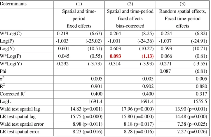
Table 2. Estimation results of cigarette demand: spatial Durbin model specification with spatial and time-period specific effects
Determinants (1) (2) (3)
Spatial and time- period fixed effects
Spatial and time-period fixed effects bias-corrected
Random spatial effects, Fixed time-period effects W*Log(C) 0.219 (6.67) 0.264 (8.25) 0.224 (6.82) Log(P) -1.003 (-25.02) -1.001 (-24.36) -1.007 (-24.91) Log(Y) 0.601 (10.51) 0.603 (10.27) 0.593 (10.71) W*Log(P) 0.045 (0.55) 0.093 (1.13) 0.066 (0.81) W*Log(Y) -0.292 (-3.73) -0.314 (-3.93) -0.271 (-3.55) Phi 0.087 (6.81) σ2 0.005 0.005 0.005 R2 0.901 0.902 0.880 Corrected R2 0.400 0.400 0.317 LogL 1691.4 1691.4 1555.5
Wald test spatial lag 14.83 (p=0.001) 17.96 (p=0.000) 13.90 (p=0.001) LR test spatial lag 15.75 (p=0.000) 15.80 (p=0.000) 14.48 (p=0.000) Wald test spatial error 8.98 (p=0.011) 8.18 (p=0.017) 7.38 (p=0.025)
LR test spatial error 8.23 (p=0.016) 8.28 (p=0.016) 7.27 (p=0.026)
To test the hypothesis whether the
spatial Durbin model
can be
simplified to the
spatial error model
, H
0
:
θ
+
δ
β
=0, one may perform
a Wald or LR test. The results reported in the second column using
the Wald test (8.98, with 2 degrees of freedom [df], p=0.011) or
using the LR test (8.23, 2 df, p=0.016) indicate that this hypothesis
must be rejected.
Similarly, the hypothesis that the
spatial Durbin model
can be
simplified to the
spatial lag model
, H
0
:
θ
=0, must be rejected
(Wald test: 14.83, 2 df, p=0.006; LR test: 15.75, 2 df, p=0.004).
This implies that both the spatial error model and the spatial lag
model must be rejected in favor of the spatial Durbin model.
Hausman's specification
test can be used to test the random effects
model against the fixed effects model. The results (30.61, 5 df,
p<0.01) indicate that the random effects model must be rejected.
Another way to test the random effects model against the fixed
effects model is to estimate the parameter "phi" (
φ
2
in Baltagi,
2005), which measures the weight attached to the cross-sectional
component of the data and which can take values on the interval
[0,1]. If this parameter equals 0, the random effects model
converges to its fixed effects counterpart; if it goes to 1, it
converges to a model without any controls for spatial specific
effects. We find phi=0.087, with t-value of 6.81, which just as
Hausman's specification test indicates that the fixed and random
effects models are significantly different from each other.
Table 1.
Estimation results of cigarette demand using different model specifications
Determinants
(1)
(2)
(3)
Non-dynamic
spatial Durbin model
no fixed effects
Non-dynamic
spatial Durbin model
with fixed effects
Dynamic
spatial Durbin model
with lag WY
t-1Intercept
2.631 (15.82)
Log(C)
-10.865 (65.04)
W*Log(C)
0.337 (11.09)
0.264 (8.25)
0.076 (2.00)
W*Log(C)
-1-0.015 (-0.29)
Log(P)
-1.251 (-21.80) -1.001 (-24.36) -0.266 (-13.19)
Log(Y)
0.554 (14.96)
0.603 (10.27)
0.100 (4.16)
W*Log(P)
0.780 (11.15) 0.093 (1.13)
0.170 (3.66)
W*Log(Y)
-0.444 (11.09) -0.314 (-3.93) -0.022 (-0.87)
R
20.435
0.902
0.977
LogL
475.5
1691.4
2623.3
Notes: t-values in parentheses
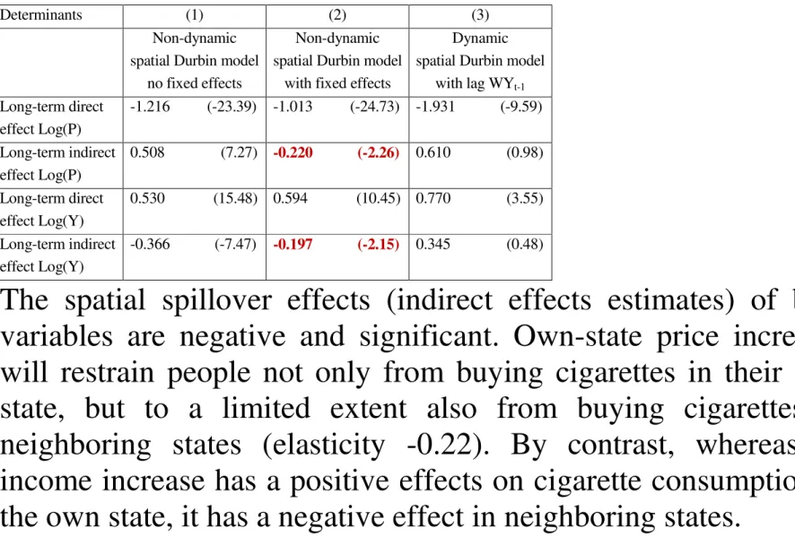
Table 2. Effects estimates of cigarette demand using different model specifications
Determinants (1) (2) (3)
Non-dynamic spatial Durbin model
no fixed effects
Non-dynamic spatial Durbin model
with fixed effects
Dynamic spatial Durbin model
with lag WYt-1 Short-term direct effect Log(P) -0.262 (-11.48) Short-term indirect effect Log(P) 0.160 (3.49) Short-term direct effect Log(Y) 0.099 (3.36) Short-term indirect effect Log(Y) -0.018 (-0.45) Long-term direct effect Log(P) -1.216 (-23.39) -1.013 (-24.73) -1.931 (-9.59) Long-term indirect effect Log(P) 0.508 (7.27) -0.220 (-2.26) 0.610 (0.98) Long-term direct effect Log(Y) 0.530 (15.48) 0.594 (10.45) 0.770 (3.55) Long-term indirect effect Log(Y) -0.366 (-7.47) -0.197 (-2.15) 0.345 (0.48)
Results non-dynamic spatial Durbin model
•
A non-dynamic spatial Durbin model cannot be used to
calculate short-term effect estimates of the explanatory
variables.
Table 2. Effects estimates of cigarette demand using different model specifications
Determinants (1) (2) (3)
Non-dynamic spatial Durbin model
no fixed effects
Non-dynamic spatial Durbin model
with fixed effects
Dynamic spatial Durbin model
with lag WYt-1 Long-term direct effect Log(P) -1.216 (-23.39) -1.013 (-24.73) -1.931 (-9.59) Long-term indirect effect Log(P) 0.508 (7.27) -0.220 (-2.26) 0.610 (0.98) Long-term direct effect Log(Y) 0.530 (15.48) 0.594 (10.45) 0.770 (3.55) Long-term indirect effect Log(Y) -0.366 (-7.47) -0.197 (-2.15) 0.345 (0.48)
The direct effects estimates of the two explanatory variables are
significantly different from zero and have the expected signs.
Higher prices restrain people from smoking, while higher income
levels have a positive effect on cigarette demand. The price
Table 1.
Estimation results of cigarette demand using different model specifications
Determinants
(1)
(2)
(3)
Non-dynamic
spatial Durbin model
no fixed effects
Non-dynamic
spatial Durbin model
with fixed effects
Dynamic
spatial Durbin model
with lag WY
t-1Log(P)
-1.251 (-21.80)
-1.001
(-24.36) -0.266 (-13.19)
Log(Y)
0.554 (14.96)
0.603
(10.27)
0.100 (4.16)
Note that these elasticities (direct effects estimates) of -1.01 and the
income elasticity to 0.594 are different from the coefficient
estimates of -1.001 and 0.603 due to feedback effects that arise as a
result of impacts passing through neighboring states and back to
the states themselves.
Table 2. Effects estimates of cigarette demand using different model specifications
Determinants (1) (2) (3)
Non-dynamic spatial Durbin model
no fixed effects
Non-dynamic spatial Durbin model
with fixed effects
Dynamic spatial Durbin model
with lag WYt-1 Long-term direct effect Log(P) -1.216 (-23.39) -1.013 (-24.73) -1.931 (-9.59) Long-term indirect effect Log(P) 0.508 (7.27) -0.220 (-2.26) 0.610 (0.98) Long-term direct effect Log(Y) 0.530 (15.48) 0.594 (10.45) 0.770 (3.55) Long-term indirect effect Log(Y) -0.366 (-7.47) -0.197 (-2.15) 0.345 (0.48)
The spatial spillover effects (indirect effects estimates) of both
variables are negative and significant. Own-state price increases
will restrain people not only from buying cigarettes in their own
state, but to a limited extent also from buying cigarettes in
neighboring states (elasticity -0.22). By contrast, whereas an
income increase has a positive effects on cigarette consumption in
The first result is not consistent with Baltagi and Levin (1992),
who found that price increases in a particular state —due to tax
increases meant to reduce cigarette smoking and to limit the
exposure of non-smokers to cigarette smoke— encourage
consumers in that state to search for cheaper cigarettes in
neighboring states.
However, whereas Baltagi and Levin’s (1992) model is dynamic, it
is not spatial; and whereas our model so far contains spatial
interaction effects, it is not (yet) dynamic.
Results: Dynamic spatial panel data model
Table 2. Effects estimates of cigarette demand using different model specificationsDeterminants (1) (2) (3)
Non-dynamic spatial Durbin model
no fixed effects
Non-dynamic spatial Durbin model
with fixed effects
Dynamic spatial Durbin model
with lag WYt-1
Short-term indirect effect Log(P)
0.160 (3.49)
The short-term spatial spillover effect of a price increase turns out
to be positive; the elasticity amounts to 0.16 and is highly
significant (t-value 3.49). This finding is in line with the original
finding of Baltagi and Levin (1992) in that a price increase in one
state encourages consumers to search for cheaper cigarettes in
neighboring states.
Table 2. Effects estimates of cigarette demand using different model specifications
Determinants (1) (2) (3)
Non-dynamic spatial Durbin model
no fixed effects
Non-dynamic spatial Durbin model
with fixed effects
Dynamic spatial Durbin model
with lag WYt-1 Short-term direct effect Log(P) -0.262 (-11.48) Short-term direct effect Log(Y) 0.099 (3.36) Long-term direct effect Log(P) -1.216 (-23.39) -1.013 (-24.73) -1.931 (-9.59) Long-term direct effect Log(Y) 0.530 (15.48) 0.594 (10.45) 0.770 (3.55)
Consistent with microeconomic theory,
the short-term direct
effects
appear to substantially smaller than
the long-term direct
effects; -0.262 versus -1.931 for the price variable and 0.099
versus 0.770 for the income variable.
Table 2. Effects estimates of cigarette demand using different model specifications
Determinants (1) (2) (3)
Non-dynamic spatial Durbin model
no fixed effects
Non-dynamic spatial Durbin model
with fixed effects
Dynamic spatial Durbin model
with lag WYt-1 Long-term direct effect Log(P) -1.216 (-23.39) -1.013 (-24.73) -1.931 (-9.59) Long-term direct effect Log(Y) 0.530 (15.48) 0.594 (10.45) 0.770 (3.55)
The long-term direct effects in the dynamic spatial Durbin model,
on their turn, appear to be greater (in absolute value) than their
counterparts in the non-dynamic spatial Durbin model; -1.931
versus -1.013 for the price variable and 0.770 versus 0.594 for the
income
variable.
Apparently,
the
non-dynamic
model
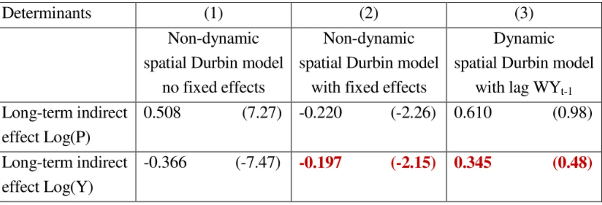
Table 2. Effects estimates of cigarette demand using different model specifications
Determinants (1) (2) (3)
Non-dynamic spatial Durbin model
no fixed effects
Non-dynamic spatial Durbin model
with fixed effects
Dynamic spatial Durbin model
with lag WYt-1 Long-term indirect effect Log(P) 0.508 (7.27) -0.220 (-2.26) 0.610 (0.98) Long-term indirect effect Log(Y) -0.366 (-7.47) -0.197 (-2.15) 0.345 (0.48)
Although greater and again positive, we do NOT find empirical
evidence that the long-term spatial spillover effect is also
significant. A similar result is found by Debarsy et al. (2011).
The spatial spillover effect of an income increase is not significant
either. A similar result is found by Debarsy et al. (2011).
Table 2. Effects estimates of cigarette demand using different model specifications
Determinants (1) (2) (3)
Non-dynamic spatial Durbin model
no fixed effects
Non-dynamic spatial Durbin model
with fixed effects
Dynamic spatial Durbin model
with lag WYt-1 Long-term indirect effect Log(P) 0.508 (7.27) -0.220 (-2.26) 0.610 (0.98) Long-term indirect effect Log(Y) -0.366 (-7.47) -0.197 (-2.15) 0.345 (0.48)