A User Manual for Benefit Cost Analysis
Using Microsoft Excel
Canesio Predo
National Abaca Research Center
Leyte State University
Baybay, Leyte, Philippines
David James
Ecoservices Pty Ltd
NSW, Australia
ECONOMY AND ENVIRONMENT PROGRAM
FOR SOUTHEAST ASIA
Canesio Predo and David James
Preface
This manual has been prepared with support provided by the Economy and Environment Programme for South East Asia (EEPSEA) to enhance the capacity of researchers in carrying out practical applications of BCA using spreadsheet modelling and analysis. The frameworks and analyses presented are based on core concepts and theory of BCA, with applications that relate primarily to environmental and natural resource management. The manual demonstrates approaches and techniques using simple examples and case studies typical of those found in most countries in the South East Asian region. Preliminary versions of the manual have been used in training programs by EEPSEA. The authors gratefully acknowledge the many useful suggestions for expansion and improvement offered by participants, now incorporated in the present version. There are several reasons for preparing a manual that relies on Microsoft Excel as the main vehicle. Excel is a powerful, user-friendly tool that helps to foster a disciplined approach to the analysis required. In BCA applications, it allows researchers to construct appropriate evaluation frameworks and carry out extensive computations easily and rapidly. Most operations can be performed by drawing on the many functions and mathematical procedures contained in Excel, including those commonly used in BCA evaluations.
The formulae, functions and results in Excel are transparent. Researchers can therefore review their work, making improvements or corrections where warranted. Resource persons providing guidance to researchers additionally have a means of seeing, in detail, how particular analyses have been carried out, enabling them to make constructive comments and suggestions, as the case may be.
One of the strongest features of Excel, as indeed with all spreadsheet software programs, is the facility to conduct simulation modelling and sensitivity analyses. An effective platform is available through which to assess the implications of changes in assumptions, variables and model parameters.
The following guidelines, instructions and worked examples have been specially designed for researchers with no prior experience in spreadsheet modelling or Excel. However, even experienced users may discover new concepts, techniques and applications to assist them in their work.
The authors encourage the interested researcher to follow the text with diligence, and reap the rewards of acquiring skills that have become essential in practical applications of BCA frameworks and methods.
I. Introduction to Excel
Microsoft Excel is a software product that falls into the general category of spreadsheets. Excel is one of several spreadsheet products that you can run on your PC.
You might have heard the terms "spreadsheet" and "worksheet". People generally use them interchangeably. To remain consistent with Microsoft and other publishers the term worksheet refers to the row-and-column matrix sheet on which you work upon and the term spreadsheet refers to this type of computer application. In addition, the term workbook will refer to the book of pages that is the standard Excel document. The workbook can contain worksheets, chart sheets, or macro modules.
Basic features of MS Excel
This guide teaches Microsoft Excel basics. Although knowledge of how to navigate in a Windows environment is helpful, this course was created for the computer novice. To begin, open Microsoft Excel. The screen shown here will appear.
We will identify the most important parts in the Microsoft Excel screen: Title bar, Menu bar, Toolbars, Worksheet, Formula bar, and Status bar.
The Title Bar -- is located at the very top of the screen. On the Title bar, Microsoft Excel displays the name of the workbook you are currently using. At the top of your screen, you should see "Microsoft Excel - Book1" or a similar name.
The Menu Bar -- is directly below the Title bar and displays the menu. The menu begins with the word File and continues with the following: Edit, View, Insert, Format, Tools, Data, Window, and Help. You use the menu to give instructions to the software. Point with your mouse to a menu option and click the left mouse button. A drop-down menu will appear. You can now use the left and right arrow keys on your keyboard to move left and right across the Menu bar options. You can use the up and down arrow keys to move up and down the drop-down menu. To select an option, highlight the item on the drop-drop-down menu and press Enter. An ellipse after a menu item signifies additional options; if you select that option, a dialog box will appear.
The Menu Bar
Do the following exercise, which demonstrates using the Microsoft Excel menu. 1. Point to the word File, which is located on the Menu bar.
2. Click your left mouse button.
3. Press the right arrow key until Help is highlighted. 4. Press the left arrow key until Format is highlighted. 5. Press the down arrow key until Style is highlighted. 6. Press the up arrow key until Cells is highlighted. 7. Press Enter to select the Cells menu option.
8. Point to Cancel and click the left mouse button to close the dialog box.
The Toolbars -- provide shortcuts to menu commands. Toolbars are generally located just below the Menu bar. The basic toolbars – Standard and Formatting – are available as the Microsoft Excel is opened. If not, follow the steps outlined below:
The Standard Toolbar
The Formatting Toolbar
1. Point to View, which is located on the Menu bar. 2. Click the left mouse button.
3. Press the down arrow key until Toolbars is highlighted.
4. Press Enter. Both Standard and Formatting should have a checkmark next to them. If both have a checkmark next to them, press Esc three times to close the menu. If either does not have a checkmark, press the down arrow key until Customize is highlighted.
5. Press Enter.
6. Point to the box or boxes next to the unchecked word or words, Standard and/or Formatting, and click the left mouse button. A checkmark should appear.
7. Note: You turn the checkmark on and off by clicking the left mouse button. 8. Point to Close and click the left mouse button to close the dialog box.
Worksheets – Microsoft Excel consists of worksheets. Each worksheet contains columns and rows. The columns are lettered A to IV; the rows are numbered 1 to 65536. The combination of column and row coordinates make up a cell address. For example, the cell located in the upper left corner of the worksheet is cell A1, meaning column A, row 1. Cell E10 is located under column E on row 10. You enter your data into the cells on the worksheet.
Empty Excel Worksheet
The Formula Bar -- If the Formula bar is turned on, the cell address displays on the left side of the Formula bar. Cell entries display on the right side of the Formula bar. Before proceeding, make sure the Formula bar is turned on.
The Formula Bar
1. Point to View, which is located on the Menu bar.
2. Click the left mouse button. A drop-down menu will appear.
3. On the drop-down menu, if Formula Bar has a checkmark next to it, the Formula bar is turned on. Press the Esc key twice to close the drop-down menu.
4. If Formula Bar does not have a checkmark next to it, press the down arrow key until Formula Bar is highlighted and press Enter. The Formula bar should appear below the toolbars.
5. Note that the current cell address displays on the left side of the Formula bar.
The Status Bar -- If the Status bar is turned on, it appears at the very bottom of the screen as shown below. Before proceeding, make sure the Status bar is turned on. The following steps will activate the Status bar:
Status Bar
1. Point to View, which is located on the Menu bar.
2. Click the left mouse button. A drop-down menu will appear.
3. On the drop-down menu, if Status Bar has a checkmark next to it, it is turned on. Press the Esc key twice to close the drop-down menu.
4. If Status Bar does not have a checkmark next to it, press the down arrow key until Status Bar is highlighted and press Enter. The Status bar should appear at the bottom of the screen.
Notice the word "Ready" on the Status bar at the lower left side of the screen. The word "Ready" tells you that Excel is in the Ready mode and awaiting your next command. Other indicators (e.g. toggle keys) appear on the Status bar in the lower right corner of the screen. Here are some examples:
• The Num Lock key is a toggle key. Pressing it turns the numeric keypad on and off. You can use the numeric keypad to enter numbers as if you were using a calculator. The letters "NUM" on the Status bar in the lower right corner of the screen indicate that the numeric keypad is on. Press the Num Lock key several times and note how the indicator on the Status bar changes.
• The Caps Lock key is also a toggle key. Pressing it turns the caps function on and off. When the caps function is on, your entry will appear in capital letters. Press the Cap Lock key several times and note how the indicator on the Status bar changes.
• Scroll Lock is another toggle key that appears on the Status bar. Pressing this key toggles the function between on and off. Scroll Lock causes the pointer movement key to move the window but not the cell pointer.
• End key allows you to jump around the screen. Pressing the End key toggles the function between on and off.
Complete the following exercise on navigating Excel. In performing this exercise make sure the Scroll Lock and End indicators are off.
1. The Down Arrow Key -- You can use the down arrow key to move downward on the screen one cell at a time.
1. Press the down arrow key several times.
2. Note that the cursor moves downward one cell at a time.
2. The Up Arrow Key -- You can use the Up Arrow key to move upward on the screen one cell at a time.
2. Note that the cursor moves upward one cell at a time.
3. The Right and Left Arrow Keys -- You can use the right and left arrow keys to move right or left one cell at a time.
1. Press the right arrow key several times. 2. Note that the cursor moves to the right. 3. Press the left arrow key several times. 4. Note that the cursor moves to the left.
4. Page Up and Page Down -- The Page Up and Page Down keys move the cursor up and down one page at a time.
1. Press the Page Down key.
2. Note that the cursor moves down one page. 3. Press the Page Up key.
4. Note that the cursor moves up one page.
5. The End Key -- The End key, used in conjunction with the arrow keys, causes the cursor to move to the far end of the spreadsheet in the direction of the arrow.
The Status Bar showing End Key 1. Press the End key.
2. Note that "END" appears on the Status bar in the lower right corner of the screen. 3. Press the right arrow key.
4. Note that the cursor moves to the farthest right area of the screen. 5. Press the END key again.
6. Press the down arrow key. Note that the cursor moves to the bottom of the screen. 7. Press the End key again.
8. Press the left arrow key. Note that the cursor moves to the farthest left area of the screen. 9. Press the End key again.
10. Press the up arrow key. Note that the cursor moves to the top of the screen.
Note: If you have entered data into the worksheet, the End key moves you to the end of the data area.
6. The Home Key -- The Home key, used in conjunction with the End key, moves you to cell A1 -- or to the beginning of the data area if you have entered data.
1. Move the cursor to column J.
2. Stay in column J and move the cursor to row 20. 3. Press the End key.
4. Press Home.
7. Scroll Lock -- Scroll Lock moves the window, but not the cell pointer.
The Status Bar showing Scroll Lock 1. Press the Page Down key.
2. Press Scroll Lock. Note "SCRL" appears on the Status bar in the lower right corner of the screen.
3. Press the up arrow key several times. Note that the cursor stays in the same position and the window moves upward.
4. Press the down arrow key several times. Note that the cursor stays in the same position and the window moves downward.
5. Press Scroll Lock to turn the scroll lock function off. 6. Press End.
7. Press Home. You should be in cell A1. Working with Cells and Ranges
A cell is a single element in a worksheet that can hold a value, text, or a formula. A cell is identified by its address, which consists of its column letter and row number. For example, cell D12 is the cell in the fourth column and the twelfth row. A group of cells is called a range. You designate a range address by specifying its upper-left cell address and its lower-right cell address, separated by a colon. Here are some examples of range addresses:
A1:B1 Two cells that occupy one row and two columns C24 A range that consists of a single cell
A1:A100 100 cells in column A
A1:D416 Cells (four rows by four columns)
C1:C65536 An entire column of cells; this range also can be expressed as C:C A6:IV6 An entire row of cells
Selecting Ranges: To perform an operation on a range of cells in a worksheet, you must select the range of cells first. For example, if you want to make the text bold for a range of cells, you must select the range and then click the Bold button on the Formatting toolbar (or, use any of several other methods to make the text bold). When you select a range, the cells appear highlighted in light blue-gray. The exception is the active cell, which remains its normal color. The figure below shows an example of a selected range in a worksheet.
Example of a selected range in a worksheet. You can select a range in several ways:
• Use the mouse to drag, highlighting the range. If you drag to the end of the screen, the worksheet will scroll.
• Press the Shift key while you use the direction keys to select a range.
• Press F8 and then move the cell pointer with the direction keys to highlight the range. Press F8 again to return the direction keys to normal movement.
• Use the Edit ÆGo To command (or press F5) and enter a range’s address manually into the Go To dialog box. When you click OK, Excel selects the cells in the range that you specified.
Selecting Complete Rows and Columns: You can select entire rows and columns in much the same manner as you select ranges, as follows:
• Click the row or column border to select a single row or column.
• To select multiple adjacent rows or columns, click a row or column border and drag to highlight additional rows or columns.
• To select multiple (nonadjacent) rows or columns, press Ctrl while you click the rows or columns that you want.
• Press Ctrl+spacebar to select a column. The column of the active cell (or columns of the selected cells) will be highlighted.
• Press Shift+spacebar to select a row. The row of the active cell (or rows of the selected cells) will be highlighted.
• Click the Select All button (or Ctrl+Shift+spacebar) to select all rows.
• Selecting all rows is the same as selecting all columns, which is the same as selecting all cells.
Selecting Noncontiguous Ranges: Most of the time, the ranges that you select will be
contiguous -- a single rectangle of cells. Excel also enables you to work with noncontiguous ranges, which consist of two or more ranges (or single cells) that are not necessarily next to each other. This is also known as a multiple selection. If you want to apply the same formatting to cells in different areas of your worksheet, one approach is to make a multiple selection. When
the appropriate cells or ranges are selected, the formatting that you select is applied to them all. A noncontiguous range selected in a worksheet is shown below:
Example of selected cells in noncontiguous ranges.
You can select a noncontiguous range in several ways:
• Hold down Ctrl while you drag the mouse to highlight the individual cells or ranges.
• From the keyboard, select a range as described previously (using F8 or the Shift key). Then, press Shift+F8 to select another range without canceling the previous range selections.
• Select Edit Æ Go To and then enter a range’s address manually into the Go To dialog box. Separate the different ranges with a comma. When you click OK, Excel selects the cells in the ranges that you specified (see Figure above).
Selecting Multisheet Ranges: The discussion so far has focused on ranges on a single worksheet. However, an Excel workbook can contain more than one worksheet. As expected, ranges can extend across multiple worksheets. Suppose that you have a workbook that is set up to track expenses by study of a large project. A common approach is to use a separate worksheet for each study, making it easy to organize the data. The figure below shows a workbook that has four sheets, named Total, Study1, Study2, and Study3. The sheets are laid out identically. The only difference is the values. The Total sheet contains formulas that compute the sum of the corresponding items in the three study worksheets.
The worksheets in the Project Expenses Summary workbook aren’t formatted in any way. Since the sheets are laid out identically, you can number formats in all the sheets simultaneously. The following is a step-by-step example of multisheet formatting:
1. Activate the Total worksheet. 2. Select the range B2:E5.
3. Press Shift and click the sheet tab labeled Study3. This selects all worksheets between the active worksheet (Totals) and the sheet tab that you click (see Figure below). Notice that the workbook window’s title bar displays [Group]. This is a reminder that you’ve selected a group of sheets and that you’re in Group edit mode.
A sample workbook with multiple worksheets selected
4. Click the Comma Style button on the Formatting toolbar. This applies comma formatting to the selected cells.
5. Click one of the other sheet tabs. This selects the sheet and also cancels Group mode; [Group] is no longer displayed in the title bar. All the worksheets in the workbook are formatted with Comma Style number format.
A sample workbook with all worksheets formatted simultaneously.
Annotating a Cell: Excel’s cell-comment feature enables you to attach a comment to a cell. This feature is useful when you need to document a particular value. It’s also useful to help you remember what a formula does.
To add a comment to a cell, select the cell and then choose InsertÆComment (or Shift+F2). Excel inserts a comment that points to the active cell, as shown in the figure below. Initially, the comment consists of your name (i.e., name of your computer). Enter the text for the cell
comment and then click anywhere in the worksheet to hide the comment. Cells that have a comment attached display a small red triangle in the upper-right corner. When you move the mouse pointer over a cell that contains a comment, the comment becomes visible.
A sample of a cell with annotation or comments.
To edit a comment, activate the cell, right-click, and then choose Edit Comment from the shortcut menu. To delete a cell comment, activate the cell that contains the comment, right-click, and then choose Delete Comment from the shortcut menu.
Filling Cells Automatically
You can use Microsoft Excel to automatically fill cells with information that occur in a series. For example, you can have word automatically fill in times, the days of the week or months of the year, years, and other types of series. The following demonstrates:
1. Type the following into the worksheet as shown.
A B C D E F G
1 1:00 Sun Sunday Jan January 2000 Type 1
2. Place the cursor in cell A1.
3. Press F8. This will anchor the cursor.
4. Press the right arrow key six times to highlight cells A1 through G1.
5. Find the small black square in the lower right corner of the highlighted area. This is called the Fill Handle.
6. Grab the Fill Handle and drag with your mouse to highlight cells A1 to G24. 7. Note how each cell fills.
2. Press Esc and then click anywhere on the worksheet to remove the highlighting.
Deleting Cell Contents: To erase the contents of a cell or range, select the cell or range and press Delete. Or, you can select Edit ÆClearÆAll. Another method is to select the cell or range of cells, right click mouse button and then select Clear Contents.
Copying, Cutting and Pasting
• Copy a cell to another cell.
• Copy a cell to a range of cells. The source cell is copied to every cell in the destination range.
• Copy a range to another range. Both ranges must be the same size.
Copying a cell normally copies the cell contents, any formatting that is applied to the original cell (including conditional formatting and data validation), and the cell comment (if it has one). When you copy a cell that contains a formula, the cell references in the copied formulas are changed automatically to be relative to their new destination.
Copying consists of two steps although shortcut methods exist:
1. Select the cell or range to copy (the source range) and copy it to the Clipboard.
2. Move the cell pointer to the range that will hold the copy (the destination range) and paste the Clipboard contents.
If you find that pasting overwrote some essential cells, choose EditÆUndo (or press Ctrl+Z). Because copying is used so often, Excel provides many different methods as follows:
Copying by using toolbar buttons: The Standard toolbar has two buttons that are relevant to copying: the Copy icon ( ) and the Paste icon ( ). Follow the steps below to copy a cell or range of cells by using toolbar buttons:
1. Highlight cell or range of cells to be copied, say A7 to B9. To do this, place the cursor in cell A7. Press F8. Press the down arrow key twice. Press the right arrow key once. A7 to B9 should be highlighted. Or highlight cell range A7 to B9 by clicking the mouse on cell A7. While holding the left mouse button at cell A7 drag it down to A9 and then to the right at B9. 2. Click on the Copy icon, which is located on the Formatting toolbar. Use the arrow key or
mouse to move the cursor to cell C7.
3. Click on the Paste icon, which is located on the Formatting toolbar 4. Press Esc to exit the Copy mode.
Copying by using menu commands: You can use the following menu commands for copying and pasting:
• Highlight cell or range of cells to be copied. Then click Edit ÆCopy -- Copies the selected cells to the Windows Clipboard and the Office Clipboard
• Click Edit Æ Paste: Pastes the Windows Clipboard contents to the selected cell or range Copying by using shortcut menus: Select the cell or range to copy (A2:B4), right-click, and then choose Copy from the shortcut menu. Then, select the cell (D2) in which you want the copy to appear, right-click, and choose Paste from the shortcut menu (see figure below).
Example showing copy and paste shortcut menus
Copying by using shortcut keys: The copy and paste operations also have shortcut keys associated with them:
• Ctrl+C: Copies the selected cells to the Clipboard
• Ctrl+V: Pastes the Clipboard contents to the selected cell or range
Copying to adjacent cells: Often, you’ll find that you need to copy a cell to an adjacent cell or range. This type of copying is quite common when working with formulas. For example, if you’re working on a budget, you might create a formula to add the values in column B. You can use the same formula to add the values in the other columns. Rather than reenter the formula, you’ll want to copy it to the adjacent cells.
Excel provides some additional options on its Edit menu for copying to adjacent cells. To use these commands, select the cell that you’re copying and the cells that you are copying to (see figure below). Then, issue the appropriate command from the following list for one-step copying:
EditÆFillÆDown (or Ctrl+D): Copies the cell to the selected range below EditÆFillÆRight (or Ctrl+R): Copies the cell to the selected range to the right EditÆFillÆUp: Copies the cell to the selected range above
To copy to adjacent cells, start by selecting the cell to copy plus the cells in which you want the copy to appear.
You also can use AutoFill to copy to adjacent cells by dragging the selection’s fill handle. Excel copies the original selection to the cells that you highlight while dragging.
Copying a range to other sheets: The copy procedures described previously also work to copy a cell or range to another worksheet, even if the worksheet is in a different workbook. Activate the other worksheet first before you select the location to which you want to copy. Follow the steps below:
• Start by selecting the range to copy. Then, press Ctrl and click the sheet tabs for the worksheets to which you want to copy the information (Excel displays [Group] in the workbook’s title bar).
• Select EditÆFillÆAcross Worksheets, and a dialog box appears that asks what you want to copy (All, Contents, or Formats).
• Make your choice and then click OK. Excel copies the selected range to the selected worksheets; the new copy will occupy the same cells in the selected worksheets as the original occupies in the initial worksheet.
Moving a cell or range: Copying a cell or range doesn’t modify the cell or range that you copied. If you want to relocate a cell or range to another location, use the EditÆCut command. This is similar to EditÆCopy command except that it also removes the contents of the selection from its original location.
To move a cell or range, therefore, requires two steps:
2. Select the cell that will hold the moved cell or range (the destination range) and paste the contents of one of the Clipboards. The destination range can be on the same worksheet or in a different worksheet—or in a different workbook.
Note that you also can move a cell or range by dragging it. Select the cell or range that you want to move and then slide the mouse pointer to any of the selection’s four borders. The mouse pointer turns into an arrow pointing up and to the left. Drag the selection to its new location and release the mouse button.
Copy and Paste Special: Excel contains two more versatile ways to paste information. You can use the Office Clipboard to copy and paste multiple items, or you can use the Paste Special dialog box to paste information in distinctive ways.
• The EditÆPaste Special command is a much more versatile version of the EditÆPaste command.
• For the Paste Special command to be available, you need to copy a cell or range to the Clipboards (using EditÆCut won’t work).
• Then, select the cell in which you want to paste, and choose EditÆPaste Special. You see the dialog box as shown below.
Paste Special Dialog box.
• The several options under Paste Special dialog box are as follows:
o Pasting all – selecting this option is equivalent to using the EditÆPaste command. It copies the cell’s contents, format, and data validation
o Pasting formulas – copies the formula of selected cell
o Pasting formulas as values – normally, when you copy a range that contains formulas, Excel copies the formulas and automatically adjust the cell references. The Value option enables you to copy the results of formulas.
o Pasting cell formats only – copy only the formatting applied in the selected cell or range to the destination cell or range.
o Pasting cell comments – copy only the cell comments from a cell or range; doesn’t copy cell contents or formatting
o Pasting validation criteria – copy the data validation command created in the selected cell or range to another cell or range
o Skipping borders when pasting – this is to avoid pasting the border of selected cell or range
o Pasting column widths – copy column width information from one column to another o Performing mathematical operations without formulas – perform an arithmetic operation
without using formulas. For example, you can copy a range to another range and select the multiply operation. Excel multiplies the corresponding values in the source range and the destination range and replaces the destination range with the new values.
o Skipping blanks when pasting – this prevents Excel from overwriting cell contents in your paste area with blank cells from the copied range.
o Transposing a range – changes the orientation of the copied range. For instance, rows become column and columns become rows. Any formulas in the copied range are adjusted so that they work properly when transposed.
Elementary Formulae
All formulas in Excel must begin with an equal sign (=). When a formula is entered into a cell, the formula itself is displayed in the formula bar when that cell is highlighted, and the result of the formula is displayed in the actual cell. When you are typing in formulas, do not type spaces; Excel will delete them.
In Microsoft Excel, you can enter numbers and mathematical formulas into cells. When a number is entered into a cell, you can perform mathematical calculations such as addition, subtraction, multiplication, and division. Use the following to indicate the type of calculation you wish to perform: + Addition - Subtraction * Multiplication / Division ^ Exponential
The following exercises demonstrate how to create formula and perform mathematical calculations.
Addition (+)
1. Move the cursor to cell A1. 2. Type 1.
3. Press Enter. 4. Type 1 in cell A2.
5. Press Enter.
6. Type =A1+A2 in cell A3. 7. Press Enter.
8. Note that cell A1 has been added to cell A2 and the result is shown in cell A3.
Place the cursor in cell A3 and look at the Formula bar. Subtraction (-)
1. Press F5. The Go To dialog box will appear. 2. Type B1.
3. Press Enter.
4. The cursor should move to cell B1. 5. Type 5 in cell B1. 6. Press Enter. 7. Type 3 in cell B2. 8. Press Enter. 9. Type =+B1-B2 in cell B3. 10. Press Enter.
11. Note that cell B1 has been subtracted from B2 and the result is shown in cell B3.
Place the cursor in cell B3 and look at the Formula bar. Multiplication (*)
1. Hold down the Ctrl key while you press “g” (Ctrl-g). The Go To dialog box will appear. 2. Type C1.
3. Press Enter. You should now be in cell C1. 4. Type 2 in cell C1.
5. Press Enter. 6. Type 3 in cell C2. 7. Press Enter.
9. Press Enter.
10. Note that C1 is multiplied by C2 and the answer is displayed in C3.
Place the cursor in cell C3 and look at the Formula bar. Division (/)
1. Press F5. 2. Type D1.
3. Press Enter. You should now be in cell D1. 4. Type 6 in cell D1. 5. Press Enter. 6. Type 3 in cell D2. 7. Press Enter. 8. Type =D1/D2 in cell D3. 9. Press Enter.
10. Note that D1 is divided by D2 and the answer is displayed in cell D3.
Place the cursor in cell D3 and look at the Formula bar.
Exponential (^) 1. Type 2 in cell B2. 2. Press Enter. 3. Type 3 in cell B3. 4. Press Enter. 5. Type =B2^B3 in cell B4. 6. Press Enter.
Place the cursor in cell B4 and look at the Formula bar.
Other Excel operations
A formula entered into a cell can consist of any of the following elements:
• Operators such as + (for addition) and * (for multiplication)
• Cell references (including named cells and ranges)
• Values or text
• Worksheet functions (such as SUM or AVERAGE)
A formula can consist of up to 1,024 characters. After you enter a formula into a cell, the cell displays the result of the formula. Here are other few examples of formulas:
=150*.05 Multiplies 150 times .05. This formula uses
only values and isn’t all that useful.
=A1+A2 Adds the values in cells A1 and A2.
=Income–Expenses Subtracts the cell named Expenses from the
cell named Income.
=SUM(A1:A12) Adds the values in the range A1:A12.
=A1=C12 Compares cell A1 with cell C12. If they are
identical, the formula returns TRUE; otherwise, it returns FALSE.
Other operators used in formulas: Excel uses variety of operators in formula. Below is the list of remaining operators used in formulas:
Operator Name
& Concatenation or join cell contents
= Logical comparison (equal to)
> Logical comparison (greater than)
< Logical comparison (less than)
>= Logical comparison (greater than or equal to) <= Logical comparison (less than or equal to) <> Logical comparison (not equal to)
Operator precedence: In an earlier example, parentheses are used in the formula, to control the order in which the calculations occur. The formula without parentheses looks like this:
=Income-Expenses*TaxRate
If you enter the formula without the parentheses, Excel computes the wrong answer. To understand why this occurs, you need to understand a concept called operator precedence, which basically is the set of rules that Excel uses to perform its calculations. Below is the list of Excels’ operator precedence.
Symbol Operator Precedence
^ Exponentiation 1 * Multiplication 2 / Division 2 + Addition 3 - Subtraction 3 & Concatenation 4 = Equal 5 < Less than 5 > Greater than 5
You use parentheses to override Excel’s built-in order of precedence. Returning to the previous example, the formula that follows doesn’t use parentheses and, therefore, is evaluated using Excel’s standard operator precedence. Because multiplication has a higher precedence, the Expense cell is multiplied by the TaxRate cell. Then, this result is subtracted from Income. This isn’t what was intended.
The correct formula, which follows, uses parentheses to control the order of operations. Expressions within parentheses are always evaluated first. In this case, Expenses is subtracted from Income and the result is multiplied by TaxRate.
=(Income-Expenses)*TaxRate
You can also nest parentheses in formulas, which means putting parentheses inside of parentheses. If you do so, Excel evaluates the most deeply nested expressions first and works its way out. The figure below shows an example of a formula that uses nested parentheses.
A formula with a nested parenthesis
This formula, =((B2*C2)+(B3*C3))*B5, has three sets of parentheses—two sets are nested inside the third set. Excel evaluates each nested set of parentheses and then adds up the two results. This sum is then multiplied by the value in B5.
Entering formulas by pointing: The formulas created earlier are entered manually. In Excel, entering formulas by pointing to cell addresses rather than entering them manually is usually more accurate and less tedious. Although this method still involves some manual typing, but you can simply point to the cell references instead of entering them manually. For example, to enter the formula =A1+A2 into cell A3, follow these steps:
1. Move the cell pointer to cell A3.
2. Type an equal sign (=) to begin the formula. Notice that Excel displays Enter in the status bar.
3. Press the up arrow twice to reach A1. As you press this key, notice that Excel displays a faint moving border around the cell and that the cell reference appears in cell A3 and in the formula bar. Also notice that Excel displays Point in the status bar.
4. Type a plus sign (+). The faint border disappears and Enter reappears in the status bar. 5. Press the up arrow one more time. A2 is added to the formula.
6. Press Enter to end the formula.
Referencing cells outside the worksheet: Formulas can refer to cells in other worksheets—and the worksheets don’t even have to be in the same workbook. Excel uses a special type of notation to handle these types of references.
• Cells in other worksheets -- To use a reference to a cell in another worksheet in the same workbook, use the following format:
SheetName!CellAddress
In other words, precede the cell address with the worksheet name, followed by an exclamation point. Here’s an example of a formula that uses a cell on the Sheet2 worksheet:
=B7*Sheet2!A1
This formula multiplies the value in cell B7 on the current worksheet by the value in cell A1 on Sheet2. If the worksheet name in the reference includes one or more spaces, you must enclose it in single quotation marks. For example, here’s a formula that refers to a cell on a sheet named All Depts (see figure below):
• Cells in other workbooks -- To refer to a cell in a different workbook, use this format: =[WorkbookName]SheetName!CellAddress
In this case, the workbook name (in square brackets), the worksheet name, and an exclamation point precede the cell address. The following is an example of a formula that uses a cell reference in the Sheet1 worksheet in a workbook named Budget:
=[Budget.xls]Sheet1!A1
If the workbook name in the reference includes one or more spaces, you must enclose it (and the sheet name) in single quotation marks. For example, here’s a formula that refers to a cell on Sheet1 in a workbook named Budget For 1999:
=B7*’[Budget For 1999]Sheet1’!A1
When a formula refers to cells in a different workbook, the other workbook doesn’t need to be open. If the workbook is closed, you must add the complete path to the reference. Here’s an example:
=B7*’C:\ Academ\BCA Course\[BCA exercise data.xls]Sheet1’!B12
Absolute vs relative references in excel formula: By default, Excel creates relative cell references in formulas except when the formula includes cells in different worksheets or workbooks. The distinction becomes apparent when you copy a formula to another cell.
• Relative references – The figure below shows a worksheet with a formula in cell D2. The formula, which uses the default relative references, is as follows:
Formula in cell D2 with relative references
When you copy this formula to the next cell below it, Excel doesn’t produce an exact copy of the formula; rather, it generates this formula:
Cell D3: =B3*C3
• Absolute references – Sometimes you dowant a cell reference to be copied verbatim. The figure below shows an example of a formula that contains an absolute reference.
Formula in cell D2 with absolute references
In this example, cell B5 contains a sales tax rate. The formula in cell D2 is as follows: =(B2*C2)*$B$5
Notice that the reference to cell B5 has dollar signs preceding the column letter and the row number. These dollar signs indicate to Excel that you want to use an absolute cell reference. When you copy this formula to the next cell below, Excel generates the following formula:
Cell D3: =(B3*C3)*$B$6
In this case, the relative cell references were changed, but the reference to cell B5 wasn’t changed, because it’s an absolute reference.
• Mixed References -- An absolute reference uses two dollar signs in its address: one for the column letter and one for the row number. Excel also allows mixed references in which only
one of the address parts is absolute. Below is a summary of all the possible types of cell references.
Example Type of Cell Reference A1 Relative reference $A$1 Absolute reference
$A1 Mixed reference (column letter is absolute) A$1 Mixed reference (row number is absolute)
The figure below shows an example of a situation in which a mixed reference is appropriate. This worksheet will contain a table of values in which each cell consists of the value in column A multiplied by the value in row 1.
The formula in cell B2 is as follows: =B$1*$A2
This formula contains two mixed cell references. In the B$1 reference, the row number is absolute, but the column letter is relative. In the $A2 reference, the row number is relative, but the column letter is absolute. You can copy this formula to the range B2:E5 and each cell will contain the correct formula. For example, the formula in cell E5 would be as follows:
=E$1*$A5
Entering nonrelative references: You can enter nonrelative references (absolute or mixed) manually by inserting dollar signs in the appropriate positions. Or, you can use a handy shortcut: the F4 key. When you’re entering a cell reference—either manually or by pointing—you can press F4 repeatedly to have Excel cycle through all four reference types.
For example, if you enter =A1 to start a formula, pressing F4 converts the cell reference to =$A$1. Pressing F4 again converts it to =A$1. Pressing it again displays =$A1. Pressing it one more time returns to the original =A1. Keep pressing F4 until Excel displays the type of reference that you want.
When you name a cell or range, Excel (by default) uses an absolute reference for the name. For example, if you give the name SalesForecast to A1:A12, the Refers to box in the Define Name dialog box lists the reference as $A$1:$A$12. This is almost always what you want. If you copy
a cell that has a named reference in its formula, the copied formula contains a reference to the original name.
Excel Functions
Microsoft Excel has a set of prewritten formulas called functions. Functions differ from regular formulas in that you supply the value but not the operators, such as +, -, *, or /. The SUM function is used to calculate sums. When using a function, remember the following: (i) Use an equals sign to begin a formula; (ii) Specify the function name; (iii) Enclose arguments within parentheses; and (iv) Use a comma to separate arguments
Here is an example of a function: =SUM(2,13,10,67) In this function:
• The equals sign begins the function,
• SUM is the name of the function
• 2, 13, 10 and 67 are the arguments
• Parentheses enclose the arguments
• A comma separates each of the arguments
In the exercises that follow, we will look at various functions. Calculating Sum (Typing the function)
1. Type 12 in cell B1. 2. Press Enter. 3. Type 27 in cell B2. 4. Press Enter. 5. Type 24 in cell B3. 6. Press Enter.
7. Type =SUM(B1:B3) in cell A4. Microsoft Excel sums cells B1 to B3. Alternatively, type = sum(, highlight the range B1:B3, type ) and press Enter
Calculating Sum (Entering a Function by Using the Menu) 1. Type 20 in cell C1.
2. Press Enter.
3. Type 30 in cell C2. 4. Press Enter.
5. Type 50 in cell C3.
6. Press Enter. Your cursor should be in cell C4. 7. Click on Insert, which is located on the Menu bar. 8. Press the down arrow key until Function is highlighted.
9. Press Enter.
10. Click on Math & Trig in the Function Category box. 11. Click on Sum in the Function Name box.
12. Click on OK.
13. Type C1:C3 in the Number1 entry field, if it does not automatically appear. 14. Click on OK.
15. Move to cell A4. 16. Type the word Sum. 17. Press Enter.
Calculating an Average
You can use the AVERAGE function to calculate an average from a series of numbers. Using the series of numbers used in calculating sum, do the following:
1. Move the cursor to cell A5. 2. Type Average.
3. Press the right arrow key. 4. Type =AVERAGE(B1:B3).
5. Press Enter. The average should appear. Calculating Min
You can use the MIN function to find the lowest number in a series of numbers. 1. Move the cursor the cell A6.
2. Type Min.
3. Press the right arrow key. 4. Type = MIN(B1:B3).
5. Press Enter. The lowest number in the series, which is 12, should appear. Calculating Max
You can use the MAX function to find the highest number in a series of numbers. 1. Move the cursor the cell A7.
2. Type Max.
3. Press the right arrow key. 4. Type = MAX(B1:B3).
5. Press Enter. The highest number in the series, which is 27, should appear.
• Formatting Text and Numbers in Excel
Format text and individual characters: To make text stand out, you can format all of the text in a cell or selected characters. Select the characters you want to format, and then click a button on the Formatting toolbar (see figure below). Thus, to boldface all text in a cell click the desired
cell and then click the Bold button. (If you had wanted to boldface only a portion of the text in a cell… Double-click to edit the cell. Then highlight the text which is to be boldfaced and click the Bold button).
Font Font size
Bold Italic Underline Align left Center Align right Merge and Center Currency Style Percent Style Comma Style Increase Decimal Decrease Increase Borders Decrease Indent Increase Indent Fill color Font color
Excel Formatting Toolbar
For example, to bold the text in cell A1, click A1 then click Bold button. The resulting text is shown below. The same procedure will be followed for changing font size, type of fonts, cell alignment (e.g., align left, center, align right), applying italic, underline fonts, and centering text or number in a cell. To merge two more cells, highlight the cells to be merged first before clicking on the merge and center icon in the formatting toolbar.
Text applied with bold attribute.
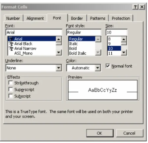
Alternatively, text formatting can also be done through the menu: Format Æ Cells then various tabs (see figure below) are available for the operation you want to make. The following are the steps for some formatting operations:
Formatting cells menu To change basic text attributes:
• Click on the name of the font you wish to use
• Click on the name of font style you want
• Click on the font size you want use Applying cell borders:
• Select the cells to receive the new border formatting.
• From the format menu, press cells.
• Choose on the borders tab
Table Border Formatting Tool
• To add a basic border outside the selected range, click on the outline button
• To add borders between cells within the selected cell range, click on the Inside button
• Click OK
Number formatting: Excel permits numbers to be formatted in many different ways. Without changing the value of the number in a cell, number formats allow numbers to be represented so that they can be used in many different kinds of projects. The steps in applying number formats through the Format Æ Cell menu.
• Select the cells containing your number(s)
• Click on the number tab
• From the list of categories, select the number format that is best suited to your project. Use the sample box to decide whether the format you chose best represents your number. Applications of financial functions and formulae in Excel
Microsoft Excel provides a series of functions destined to perform various types of financially related operations. These functions use common factors depending on the value that is being calculated. Many of these functions deal with investments or loan financing. The Financial functions therefore are designed to perform calculations that involve money. This manual will focus only on selected financial functions.
• Loan and annuity functions – Listed below are functions that can help you perform calculations related to loans and annuities. Notice that these functions all use pretty much the same arguments—although the exact arguments that are used depend on the function.
List of loan and annuity functions.
Function Calculation Arguments
FV Future value Rate, Nper, Pmt, [PV], [Type]
PV Present value Rate, Nper, Pmt, [FV], [Type]
PMT Payment Rate, Nper, PV, [FV], [Type]
PPMT Principal payment Rate, Per, Nper, PV, [FV], [Type]
IPMT Interest payment Rate, Per, Nper, PV
ISPMT Payment interest Rate, Per, Nper, PV
RATE Interest rate per period Nper, Pmt, PV, [FV], [Type], [Guess]
NPER Number of periods Rate, Pmt, PV, [FV], [Type]
* Arguments in brackets are optional
To use these functions successfully, you must understand how to specify the arguments correctly. The following list explains these arguments:
Nper: Total number of payment periods. For a 30-year mortgage loan with monthly payments, Nper is 360.
Per: Period in the loan for which the calculation is being made; it must be a number between 1 and Nper.
Pmt: Fixed payment made each period for an annuity or a loan. This usually includes principal and interest (but not fees or taxes).
FV: Future value (or a cash balance) after the last payment is made. The future value for a loan is 0. If FV is omitted, Excel uses 0.
Type: Either 0 or 1, and indicates when payments are due. Use 0 if the payments are due at the end of the period, and 1 if they are due at the beginning of the period.
Guess: Used only for the RATE function. It’s your best guess of the internal rate of return. The closer your guess, the faster Excel can calculate the exact result.
The Future Value of an Investment (FV): FV returns the future value of an investment based on periodic, constant payments and a constant interest rate. To calculate FV, you can use the FV() function. The syntax of this function is:
FV(rate,nper,pmt,pv,type) where:
Rate = is the interest rate per period.
Pv = is the present value, or the lump-sum amount that a series of future payments is worth right now. If pv is omitted, it is assumed to be 0 (zero), and you must include the pmt argument.
Nper, Pmt = are similarly defined above. Remarks
• Make sure that you are consistent about the units you use for specifying rate and nper. If you make monthly payments on a four-year loan at 12 percent annual interest, use 12%/12 for rate and 4*12 for nper. If you make annual payments on the same loan, use 12% for rate and 4 for nper.
• For all the arguments, cash you pay out, such as deposits to savings, is represented by negative numbers; cash you receive, such as dividend checks, is represented by positive numbers.
Steps to Calculate FV:
2. Save it as Financial Function Examples.xls.
3. Double-click Sheet1 to put its label into edit mode. Type Future Value and press Enter. 4. Click cell B8 and, on the main menu, click Insert -> Function...
5. In the Paste Function dialog box, in the Function Category list, click Financial. In the Function Name list, double-click FV and move the FV window so you can see the values on the worksheet.
6. Click the box to the right of Rate and, on the worksheet, click cell B3 and type /12 7. In the FV window, click the box to the right of Nper and, on the worksheet, click cell B4. 8. In the FV window, click the box to the right of Pmt and type – then click cell B5.
9. In the FV window, click the box to the right of Pv and type – then click B6.
10. Since this is a loan, the payments are expected at the end of the month. Therefore, in the FV window, click the box to the right of Type and type 0.
Investment or Loan Payment (PMT): The PMT() function is used to calculate the regular payment of loan or an investment. Its syntax is:
PMT(rate,nper,pv,fv,type)
In the following example, a farmer is applying for a tractor loan. The cost of the tractor will be entered in cell C4. It will be financed at a rate entered in cell C6 for a period set in cell C7. The dealer estimates that the tractor will have a value of $0.00 when it is paid off.
Steps to calculate PMT:
1. Double-click Sheet3 to put it in edit mode. Type Payments Amount and press Enter 2. Complete the worksheet as shown in the figure below
3. Click cell C6 and type /12, 4. Click cell C7 and type ,- 5. Click cell C4 and type , 6. Click cell C5 and type, 0)
7. On the Formula Bar, click the Enter button or press Enter key
Example of PMT function to compute monthly loan payments.
Number of Periods for an Investment (Nper): The NPER() function returns the number of periods for an investment based on periodic, constant payments and a constant interest rate. It’s syntax is:
NPER(rate, pmt, pv, fv, type)
To calculate NPER, follow and complete the worksheet shown below. The formula in cell B9 is =NPER(B3/12,-B4,-B5,B6,1).
Example of NPER function to calculate number of payments.
The IPMT() function: Returns the interest payment for a given period for an investment based on periodic, constant payments and a constant interest rate. Its syntax is
IPMT(rate,per,nper,pv,fv,type)
Example: Suppose you are applying for a housing loan and the bank decides (or agrees with you) that the loan will be spread over 5 years (5 years * 12 months each = 60 months). The bank then applies a certain interest rate. The IPMT() function can help you calculate the amount of interest that the lending institution would earn during a certain period. For example, you can use it to know how much money the bank would earn in the 3rd year, or the 4th year, or the 1st year. Based on this, this function has an argument called Period, which specifies the year you want to find out the interest earned in.
Follow the worksheet below to compute for IPMT. The formula for cell B8 is: =IPMT(B4/12,B5,B6,-B3)
Example of IPMT function to calculate periodic interest earned.
The Principal Payment or the Amount Paid on the Principal: The PPMT() function returns the payment on the principal for a given period for an investment based on periodic, constant payments and a constant interest rate. Its syntax is
PPMT(rate,per,nper,pv,fv,type)
Using the same example in IPMT, the formula in B9 for computing the principal payment is (see also figure below):
=PPMT(B4/12,B5,B6,-B3)
Example of PPMT function to calculate principal payment.
The Present Value (PV): The PV() function returns the present value of an investment. The present value is the total amount that a series of future payments is worth now. For example, when you borrow money, the loan amount is the present value to the lender. Its syntax is:
PV(rate,nper,pmt,fv,type)
Note that payments are annuity or same for every period. This is the difference between PV and NPV function, which will be discussed later.
To calculate PV, follow the worksheet below. The formula for computing PV in cell B6 is: =PV(B4/12,B5*12,-B3,0)
Example of PV function calculation.
Interest Rate: The RATE() function returns the interest rate per period of an annuity. RATE is calculated by iteration and can have zero or more solutions. If the successive results of RATE do
not converge to within 0.0000001 after 20 iterations, RATE returns the #NUM! error value. Its syntax is:
RATE(nper,pmt,pv,fv,type,guess)
An example on how to compute for interest rate of an annuity is given below. Follow exactly the worksheet below for the formula to work correctly. Cells B6 and B7 show the formulas for the annual rate of the loan and the monthly rate interest, respectively:
B6: =RATE(B3*12,-B4,B5)*12 B7: =RATE(B3*12,-B4,B5)
Example of RATE function calculation.
II. Basic Excel Operations in BCA
Financial Functions and Formulae used in BCA
The financial functions and formulae used in evaluating investment or project worth from efficiency criteria are: net present value (NPV), internal rate of return, and benefit cost ratio (BCR). Whether you are doing financial analysis or economic analysis, the same functions and formulae are used in the calculating those project worth measures. The difference lies on the prices being used and the components included in the calculus of costs and benefits. Market prices are used in the financial analysis to determine project or investment profitability from the investor’s or individual’s point of view. On the other hand, economic prices or shadow prices are used in economic analysis to determine the desirability of the project from the society’s point of view. The costs of externalities arising from the project are also included in economic analysis. The relevant functions in Excel are described as financial functions and some of them are especially important in BCA. But when used in BCA they may have a different conceptual basis. If a financial analysis is required as a complement to a BCA, some additional financial formulae in Excel are useful – but these will be dealt with in a later section of the guidebook.
The Net Present Value (NPV): The NPV function returns the net present value of an investment based on a series of periodic cash flows and a discount rate. The net present value of
an investment is today's value of a series of future payments (negative values) and income (positive values). Its syntax in Excel is:
=NPV(rate, value1, value2, ...)
where:
Rate is the rate of discount over the length of one period.
Value1, value2,... are 1 to 29 arguments representing the payments and income. Value1, value2,... must be equally spaced in time and occur at the end of each period.
NPV uses the order of value1, value2,... to interpret the order of cash flows. Be sure to enter your payment and income values in the correct sequence. Arguments that are numbers, empty cells, logical values, or text representations of numbers are counted; arguments that are error values or text that cannot be translated into numbers are ignored. If an argument is an array or reference, only numbers in that array or reference are counted. Empty cells, logical values, text, or error values in the array or reference are ignored.
Remarks: The NPV investment begins one period before the date of the value1 cash flow and ends with the last cash flow in the list. The NPV calculation is based on future cash flows. If your first cash flow occurs at the beginning of the first period, the first value must be added to the NPV result, not included in the values arguments.
NPV is similar to the PV function (present value). The primary difference between PV and NPV is that PV allows cash flows to begin either at the end or at the beginning of the period. Unlike the variable NPV cash flow values, PV cash flows must be constant throughout the investment. NPV is also related to the IRR function (internal rate of return). IRR is the rate for which NPV equals zero: NPV(IRR(...), ...)=0.
Examples of NPV Computation:
1. Suppose you're considering an investment in which you pay $10,000 one year from today and receive an annual income of $3000, $4200, and $6800 in the three years that follow. Assuming an annual discount rate of 10 percent, the net present value of this investment is:
=NPV(10%, -10000, 3000, 4200, 6800) equals $1188.44
In the preceding example, you include the initial $10,000 cost as one of the values, because the payment occurs at the end of the first period. This setup does not use Excel cell reference and hence it is not very useful when sensitivity analysis is made.
2. In this example we will use cell reference. Consider an investment that starts at the beginning of the first period. Suppose you're interested in putting up of a shoe store. The investment cost of the business is $40,000, and you expect to receive the following income for the first five years of operation: $8000, $9200, $10,000, $12,000, and $14,500. The annual discount
rate is 8%. This might represent the rate of inflation or the interest rate of a competing investment.
The cost and income figures from the shoe store are entered in B3 through B8 respectively, and the annual discount rate is entered in B9 (see figure below), then the net present value of the shoe store investment is given by:
NPV: =NPV($B$9, B4:B8)+B3 equals $1,922.06
Example of NPV function calculation.
In the preceding example, you don't include the initial $40,000 cost (B3) as one of the values in the NPV function, because the payment occurs at the beginning of the first period. It is entered separately in the equation in undiscounted form.
Present Value (PV) of an Annuity: As mentioned earlier this function is similar to NPV function except that PV allows cash flows to begin either at the end or at the beginning of the period. Unlike the variable NPV cash flow values, PV cash flows must be constant throughout the investment period. The formula to compute PV of an annuity is:
Present Value of Payments = PV of Annuity Factor X Annuity
= xA r r r n n ) 1 ( 1 ) 1 ( + − +
where r is the discount rate, n is the time horizon of the investment and A is annual equal payments. The syntax in Excel for PV as defined above is =PV(rate,nper,pmt,fv,type).
Examples of present value of annuity calculation using Excel is shown below. Three ways of calculating present value of annuity are presented: (i) by discounting each annual payment and get the sum over the investment period, (ii) by using the annuity factor formula, and (iii) by using Excel built-in PV function. The PV of an annuity is computed in three ways using Excel as follows:
a) By discounting each annual payment
1. Enter the discount rate and the annuity payments in the cells indicated in the worksheet.
2. Calculate the discount factor (DF) per year using the formula: DF = 1/(1+r)n. The Excel formulae per year are as follows:
Year 1: = 1/(1+ $B$3)^B5; Year 2: = 1/(1+ $B$3)^C5; Year 3: = 1/(1+ $B$3)^D5 Year 4: = 1/(1+ $B$3)^E5; Year 5: = 1/(1+ $B$3)^F5
3. Multiply the DF with annual payment and then get the sum to obtain the PV of annuity payment. The Excel formula at cell B10 is: =SUM(B8:F8).
b) By using annuity factor formula
1. At cell B13 enter the formula for calculating the PV of annuity factor as follows: =((1 + $B$3)^F5 - 1)/($B$3*(1 + $B$3)^F5)
2. Calculate PV of annuity at cell B14 with this formula: =B6*B13
c) By PV function in Excel. For this method, enter the formula in cell B17 as follows: B17: =PV($B$3,5,1200)*-1
The Present Value of a Perpetuity or Capitalization Ratio: When an annuity continues indefinitely, it is called a perpetuity. The present value of A received (at the end of) each period in perpetuity at r discount rate is given by:
Capitalization Ratio = A/r
For example, the present value of a perpetuity of $1,200 per year when the discount rate is 8 percent is $12,000. Calculated using Excel at cell C7 in the worksheet shown below, the formula is =C3/C4.
Internal Rate of Return (IRR): The IRR function returns the internal rate of return for a series of cash flows represented by the numbers in values. These cash flows do not have to be even, as they would be for an annuity. However, the cash flows must occur at regular intervals, such as monthly or annually. The internal rate of return is the interest rate received for an investment consisting of payments (negative values) and income (positive values) that occur at regular periods. Its syntax is given by:
IRR(values, guess) where:
Values= is an array or a reference to cells that contain numbers for which you want to calculate the internal rate of return.
• Values must contain at least one positive value and one negative value to calculate the internal rate of return.
• IRR uses the order of values to interpret the order of cash flows. Be sure to enter your payment and income values in the sequence you want.
• If an array or reference argument contains text, logical values, or empty cells, those values are ignored.
Guess= is a number that you guess is close to the result of IRR.
• Microsoft Excel uses an iterative technique for calculating IRR. Starting with guess, IRR cycles through the calculation until the result is accurate within 0.00001 percent. If IRR can't find a result that works after 20 tries, the #NUM! error value is returned.
• In most cases you do not need to provide guess for the IRR calculation. If guess is omitted, it is assumed to be 0.1 (10 percent).
• If IRR gives the #NUM! error value, or if the result is not close to what you expected, try again with a different value for guess.
Using the preceding example, the IRR computation is shown in the figure below and as given by the formula:
IRR: =IRR(B3:B8,0.15) equal 10%
Example of IRR function calculation.
Benefit Cost Ratio (BCR): The BCR is the ratio of discounted stream of benefits and discounted stream of costs over the lifetime of the project. Unfortunately, there is no BCR function in Excel. However, this measure can be calculated through Excel formula. The step-by-step procedure for computing BCR is provided in the simple BCA exercise below.
Practice Exercise: Simple BCA Proposed Irrigation Project
1. Enter the information in the spreadsheet below. Be sure that the information is entered in the same cells as given, or the formulas will not work. The information is the stream of costs and benefits (in millions) estimated for a proposed irrigation project. All costs such as initial investment costs, operating and maintenance costs are incurred at the end of each year. The benefits are the revenues from sales of irrigation water at the end of each year.
2. To determine the desirability of the project from an efficiency criterion, first calculate the Net Benefit for each year of the project. To do this, enter the following formula.
D5: =B5-C5
4. Second, calculate the discount factor for each year. Enter the following formula. E5: =1/(1+$H$1)^A5
5. Copy the formula in cell E5 to the cell range E6:E14.
6. Calculate the Present Value for each year by multiplying the total benefit for each year by the discount factor for each year. Enter the following formula:
F5: =D5*E5
7. Copy the formula in cell F5 to the cell range F6:F14.
8. Find the Net Present Value. Add together the Present Values for each year. Enter the following formula:
F16: =sum(F5:F14)
Note: Steps 6-8 could be accomplished with one simple formula: =sumproduct(D5:D14,E5:E14)
8. An easy way of calculating net present value can replace steps 4-8. Excel has a net present value function as follows: =NPV(rate,value1,value2,...). This function assumes that each value occurs at the end of consecutive years (i.e., year1,year 2, year 3,...) since all discounting in Excel assumes that amounts refer to the end of each time period. As such we would normally begin with time period t = 1. For this exercise enter the following formula:
F17. =npv(H1,D5:D14)
9. A usual piece of information for a benefit cost analysis is the discount rate that returns a net present value of 0. This can be obtained with the IRR function [=irr(values,guess value)]. For this exercise enter the following formula:
F18: =irr(D5:D14,0.15)
10. Another measure used in BCA is the benefit cost ratio. This can be obtained by dividing the discounted benefits (i.e., PV Benefits at a given discount rate) by the discounted cost. For this exercise enter the following formula:
F19: =npv(H1,B5:B14) F20: =npv(H1,C5:C14) F21: =F19/F20
Your completed spreadsheet should look like the one below. Save the spreadsheet as “BCAExer1.xls”
It is suggested to set up the data with time period begins at t=1. However, in the case where time period begins with t=0 instead of t=1, there is a need to modify the NPV formula that uses the NPV Excel function. Using the same data above, the cost at year 0 represents the initial investment while costs for years 1-9 are the maintenance and operating costs incurred at the end of each year. Setting up the data this way, it is assumed that the initial investment costs occur at
the beginning of the project and not at the end of year 1. Thus, these initial costs are not to be discounted and have to be added on to the result returned by the NPV function computed for years 1-9. For this conceptual difference, the NPV formula in cell F17 is changed from =npv(H1,D5:D14) to =npv(H1,D6:D14)+D5. Likewise, the formula for the PV of Benefit is changed from =npv(H1,B5:B14) to =npv(H1,B6:B14)+B5 while for the PV of Cost is changed from =npv(H1,C5:C14) to =npv(H1,C6:C14)+C5. The modified BCA worksheet calculation reflecting these changes is shown below:
Sensitivity Analysis: In a typical sensitivity analysis, the value of an input variable identified as a significant potential source of uncertainty is changed (either within some percentage of the initial value or over a range of reasonable values) while all other input values are held constant, and the amount of change in analysis results is noted. This sensitivity process is repeated for other input variables for which risk has been identified. The input variables may then be ranked according to the effect of their variability on BCA results.
Sensitivity analysis, therefore, allows the analyst to get a feel for the impact of the variability of individual inputs on overall economic results. If the sensitivity analysis reveals that reasonable changes in an uncertain input variable will not change the relative economic ranking of project alternatives or undermine the project’s economic justification, then the analyst can have reasonable comfort that the results are robust.
A sensitivity analysis will be conducted for the data that begins at t=1. To systematically perform sensitivity analysis in Excel, summarize the different sensitivity scenarios in tabulated form (as