On the Regularity of Optimal Dynamic Blocking
Strategies
Alberto Bressan and Maria Teresa Chiri Department of Mathematics, Penn State University
University Park, Pa. 16802, USA. e-mails: [email protected], [email protected].
December 3, 2020
Abstract
The paper studies a dynamic blocking problem, motivated by a model of optimal fire confinement. While the fire can expand with unit speed in all directions, barriers are constructed in real time. An optimal strategy is sought, minimizing the total value of the burned region, plus a construction cost. It is well known that optimal barriers exists. In general, they are a countable union of compact, connected, rectifiable sets. The main result of the present paper shows that optimal barriers are nowhere dense. The proof relies on new estimates on the reachable sets and on optimal trajectories for the fire, solving a minimum time problem in the presence of obstacles.
Keywords: Dynamic blocking problem, minimum time problem with obstacles.
Mathematics Subject Classification: 49Q20, 34A60, 49J24, 93B03.
1
Introduction
We consider the dynamic blocking problem introduced in [3], for a model of wildfire propaga-tion [17]. To restrict the spreading of the fire, it is assumed that a barrier can be constructed, in real time. This could be a thin strip of land which is either soaked with water poured down from a helicopter, or cleared from all vegetation using a bulldozer, or sprayed with fire extinguisher by a team of firemen. In all cases, the fire will not cross that particular strip of land. Here the key point is that the barrier is being constructed at the same time as the fire front is advancing.
In this setting, a natural problem is to find the best possible strategy. In other words, we seek the optimal location of the barriers, in order to minimize:
[total value of the burned area] + [total cost for constructing the barriers] (1.1) among all barriers that can be constructed in real time.
We consider here the simplest situation where the fire initially burns on an open setR0, and
propagates with unit speed in all directions. We assume
(A1) The initial setR0⊂R2 is open, bounded, nonempty, connected, with Lipschitz boundary
∂R0.
If barriers are not present, for eacht≥0 the setR(t) reached by the fire is defined as R(t) =.
x(t) ; x(·) is 1-Lipschitz, x(0)∈R0
= x∈R2; d(x, R0)< t .
(1.2)
Here and in the sequel, by 1-Lipschitz we mean a function with Lipschitz constant 1. Moreover, d(x,Ω) denotes the distance of a point x to the set Ω⊂R2, whileh·,·iis the Euclidean inner
product in R2. The closure and the boundary of Ω are denoted by Ω and ∂Ω respectively.
By B(x, r) we denote the open ball centered at x with radius r. More generally, for Ω⊂R2,
B(Ω, r) = {x; d(x,Ω) < r} denotes the open neighborhood of radius r around Ω. Finally, m1, m2 denote the 1-dimensional and 2-dimensional Hausdorff measure, respectively.
Next, we assume that the spreading of the fire can be controlled by constructing a barrier.
Definition 1.1. AbarrierΓ⊂R2 is a disjoint union of countably many compact connected, rectifiable sets, with finite total length.
Throughout the following, we write
Γ = [
i≥1
Γi (1.3)
to denote a barrier, as a union of its compact, rectifiable, connected components.
Intuitively, we think of a barrier as a family of curves in the plane, which the fire cannot cross. When a barrier Γ is in place, the set reached by the fire is reduced. This leads to the definition of the new reachable set
RΓ(t)=. nx(t) ; x(·) is 1-Lipschitz, x(0)∈R0, x(τ)∈/Γ for all τ ∈[0, t] o
. (1.4)
Clearly, in this case the burned set will be somewhat smaller: RΓ(t) ⊆R(t) for everyt ≥0. Since in our model the barrier is constructed at the same time as the fire propagates, a restriction on its length must be imposed.
Definition 1.2. Given a construction speed σ >1, we say that the barrier Γ is admissible
if
m1 Γ∩RΓ(t)
≤ σt for all t≥0. (1.5)
Remark 1.3. For eacht≥0, the set
γ(t) = Γ. ∩RΓ(t)
appearing in (1.5) is the part of the barrier Γ touched by the fire at timet. This is the portion that actually needs to be put in place within timet, in order to restrain the fire. The remaining portion Γ\γ(t) can be constructed at a later time. This motivates the above definition. The equivalence between different formulations of the dynamic blocking problem was proved in [8].
Fire propagation can equivalently be described in terms of the minimum time function TΓ(x) = inf.
t≥0 ; x∈RΓ(t) . (1.6)
From the definition, it follows that TΓ is lower semicontinuous. We think of TΓ(x) as the minimum time needed for the fire to reach the pointx, starting fromR0 and without crossing
the barrier. Notice thatTΓ(x) = +∞if the fire never reaches a neighborhood ofx. In general, the minimal time function TΓ can be computed by solving a Hamilton-Jacobi equation with obstacles, namely
|∇T(x)| = 1 x /∈Γ, (1.7)
T(x) = 0 if x∈R0. (1.8)
For a precise definition and properties of this solution, see [13]. We recall that TΓ is locally an SBV function [1]. The set where it has jumps is contained inside Γ. If the functionTΓ is known, we can then recover the regionRΓ(t) burned within time tas
RΓ(t) =
x∈R2; TΓ(x)≤t .
Two mathematical problems can now be formulated.
(BP) Blocking Problem. Given a bounded open set R0, decide whether there exists an
admissible barrier Γ such that the entire region burned by the fire RΓ∞ =.
[
t>0
RΓ(t) (1.9)
is bounded.
(OP) Optimization Problem. Given an initial set R0 and a constant c0 ≥ 0, find an
admissible barrier Γ which minimizes the total cost
J(Γ) =. m2 RΓ∞
+c0m1(Γ). (1.10)
Remark 1.4. For a given initial domain R0, the set RΓ∞ in (1.9) burned by the fire can be
characterized as the union of all connected components ofR2\Γ which intersectR0. For any
bounded open setR0, it is known [3,4,5,9] that a blocking strategy exists if the construction
speed isσ >2, while it does not exist ifσ≤1. The existence of a blocking strategy forσ∈]1,2] is a challenging open problem. See the review [4] for a more comprehensive discussion. In a very general setting, the existence of an optimal barrier was proved in [6, 13]. Under the assumption that this optimal barrier is the union of finitely many Lipschitz arcs, various necessary conditions were derived in [3, 10, 18]. Indeed, assuming Lipschitz regularity, one can reformulate the problem in the classical setting of the Calculus of Variations, or within the theory of optimal control [7,12,15]. Necessary conditions for optimality are thus obtained in terms of the Euler-Lagrange equations, or by applying the Pontryagin Maximum Principle. For example, when the initial setR0 is a circle and the construction speed isσ >2, among all
simple closed curves, it is known that the admissible barrier that encloses the smallest burned area is the union of an arc of circumference and two logarithmic spirals [11].
Unfortunately, the results in [6,13] only provide the existence of an optimal barrier Γ∗ with the minimal regularity properties stated in Definition1.1. Namely, we only know that Γ∗ is the union of countably many compact, connected, rectifiable sets. It remains an outstanding open problem to close this gap, establishing further regularity properties of the optimal barrier, so that necessary conditions for optimality can then be applied. In the present paper we take a step in this direction. Our main goal is to prove
Theorem 1.5. For the optimization problem (OP), any optimal barrierΓ is nowhere dense.
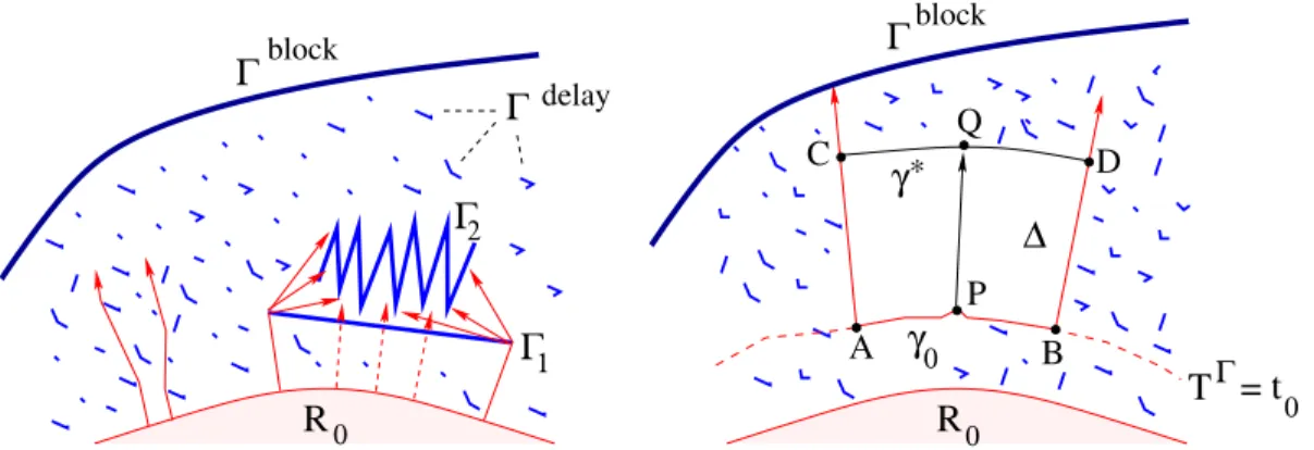
This result is motivated by the following considerations. As shown in Fig.1, left, the optimal barrier can be split as
Γ = Γblock∪Γdelay. Here Γblock = ∂RΓ
∞ is the portion which actually separates the burned region from the
un-burned one. On the other hand, Γdelay accounts for the walls whose only purpose is to delay the advancement of the fire front. Eventually, these walls are encircled by the fire on both sides.
We recall that the fire propagates with speed 1, while the barrier is constructed at speedσ >1. Building a connected component Γ1 of the barrier, with length `1, thus requires an amount
of time τ1 = `1/σ. On the other hand, the fire needs up to time `1 in order to completely
surround Γ1. In some cases, it can thus be an advantage to construct some barriers with the
sole purpose of slowing down the propagation of the fire.
At an intuitive level, however, building a barrier which contains a large number of very small connected components should be ineffective, because the fire can quickly get around each connected portion. To prove Theorem 1.5, we need to show that a collection of walls which is dense on an open set cannot be optimal. Indeed, some of these walls should be removed, because the time needed to build them is longer than the amount by which they delay the advancement of the fire front.
The heart of the matter is to understand which portions of the barrier can be removed. As shown in Fig. 1, left, the connected component Γ1 delays the advancement of the fire front.
If we remove Γ1, then we do not have enough time to construct Γ2. Hence, to achieve an
admissible barrier Γ0 ⊆Γ\Γ1 satisfying (1.5), we should also remove the component Γ2. In
turn, this may force us to remove further components Γ3,Γ4, . . . If at the end of this process
we need to remove the outer component Γblock as well, then the entire construction fails. Toward a proof of Theorem 1.5, we shall construct a “flow box” ∆, as shown in Fig. 1, right. Here the lower boundary coincides with the location of the fire front at some timet0>0. The
two sides are straight lines, consisting of optimal trajectories for the fire which do not intersect any of the barriers. The upper boundary is a curve γ∗, consisting of points having a fixed distance h > 0 fromγ0. These are the points that the fire would reach at time t∗ = t0 +h,
if no barriers were present. A careful analysis will show that, by removing all the barriers contained inside ∆, the remaining portion Γ♦ = Γ\∆ is still admissible, and achieves a lower total cost (1.10).
The remainder of the paper is organized as follows. Section2is concerned with the minimum time problem for the fire, in the presence of barriers. The first main result, Lemma 2.2, considers a path ξ that crosses some of the connected components Γi of the barrier. By
t block Γ delay γ γ Γ ∆ Γblock 0 0 R0 R0 Γ1 Γ2 Γ P C ∗ Q T = D B A
Figure 1: Left: if the connected component Γ1 of the barrier is removed, then there is not enough
time to construct Γ2, before the fire reaches it. Right: by removing all barriers inside a carefully chosen
“flow box” ∆, the remaining portion Γ♦ = Γ\∆ still form an admissible barrier, blocking the fire within the same region as before and yielding a smaller total cost.
inserting additional loops, we prove the existence of a modified path ˜ξ which starts and ends at almost the same points as ξ, and does not touch the barrier. Moreover, the difference between the lengths of the two paths is no greater than the total length P
im1(Γi) of the
components which were crossed. The second main result of this section, Lemma 2.4, shows that the set of times where the fire front touches a component Γi is contained in an interval
[ai, bi] of length bi−ai ≤m1(Γi). Moreover, when no barrier is touched, the set reached by
the fire expands with unit speed in all directions. All these results are intuitively obvious when Γ contains finitely many compact, connected components. However, if Γ is the union of countably many components, possibly everywhere dense, a more careful proof is needed. In Section 3 we prove some lemmas describing how the minimum time function TΓ in (1.6) changes when the barrier Γ is perturbed. This analysis is useful, because it allows us to approximate an arbitrary barrier with a polygonal one.
Section 4 continues the study of optimal trajectories for the fire, reaching points x ∈ R2 in
minimum time without crossing the barrier Γ. The key result in this section (Lemma 4.1) shows that, if the total length of all barriers is small, most of these optimal trajectories for the fire contain long straight segments. This fact can be rigorously stated in terms of an integral inequality. The proof is first achieved in the case of polygonal barriers. The general case follows by an approximation argument.
Section5contains another key estimate. Roughly speaking, Lemma5.5shows that, if a barrier Γ is “ε-sparse”, then the additional time needed by the fire to go around it is bounded by 9ε m1(Γ). We observe that the time needed to construct this barrier isσ−1m1(Γ), whereσ is
the construction speed. Ifε >0 is sufficiently small, the time needed to construct this portion of barrier is not compensated by its effectiveness in delaying the advance of the fire front. One can thus conclude that the barrier is not optimal.
The proof of Theorem1.5is then completed in Section6. It consists of two main steps. First, we use Lemma4.1 to construct a “flow box” ∆, as shown in Fig.1, whose sides are segments contained in optimal trajectories for the fire which do not cross the barrier Γ. We then use Lemma5.5and show that, by removing all the portions of the barrier contained inside ∆, one obtains a new admissible barrier Γ♦= Γ\∆, which yields a smaller total cost.
2
Optimal trajectories for the fire
In this section we focus on the optimization problem for the fire. LetR0⊂R2 be a bounded,
connected open set, and let Γ = ∪iΓi be a barrier, consisting of countably many compact,
rectifiable, connected components, with finite total length. We seek trajectories that, starting from the closure R0, reach points x ∈R2 in minimum time, without crossing Γ. To achieve
the existence of these optimal trajectories, referring to Fig.2 we introduce
Definition 2.1. A trajectory for the fire t7→x(t), t∈[0, T], is admissible if there exists a sequence of 1-Lipschitz trajectories t7→xn(t) such that
xn(0)∈R0, xn(t)∈/ Γ for all t∈[0, T], (2.1)
and moreoverxn(t)→x(t) uniformly on [0, T], asn→ ∞.
We say that a trajectory t7→ x(t) does not touch the barrier Γ if x(t) ∈/ Γ for all times
t≥ 0. If x(·) is the uniform limit of trajectories xn(·) that do not touch Γ, we say that x(·)
does not cross the barrier Γ.
(t) (t) x ~ (t) x xn Γ R0
Figure 2: The trajectory t 7→ x(t) touches the barrier Γ, but does not cross it. Indeed, it can be obtained as a uniform limit of trajectories xn(·) that do not touch Γ. On the other hand, the trajectory ˜x(·) is not admissible: it goes right across the barrier.
Given a point ¯x ∈ R2, we seek an admissible trajectory t 7→ x(t) which starts from a point
in the closureR0 and reaches ¯x in minimum time without crossing Γ. If ¯x can be reached in
finite time, the existence of such an optimal trajectory is straightforward. Indeed, define Tinf = lim.
ε→0 h
infimum time needed to reach a point in the ballB(¯x, ε), starting from R0 and without touching the barrier Γ
i
.
Let xn : [0, Tn] 7→ R2 be a minimizing sequence of 1-Lipschitz trajectories, satisfying (2.1)
together with
xn(Tn) → x,¯ Tn → Tinf as n→ ∞.
By taking a subsequence we can assume the uniform convergence xn → x, for some limit
function x : [0, Tinf] 7→ R2. According to Definition 2.1, this limit trajectory is admissible.
Hence it provides an optimal solution.
Given a trajectory ξ : [0, τ] 7→ R2 that crosses part of the barrier, the next lemma provides
the key tool for constructing trajectories that “loop around” each connected component, and reach almost the same endpoint without touching Γ.
Lemma 2.2. Consider a barrierΓ =∪i≥1Γi, written as the union of its connected components.
Assume thatR2\Γ is connected. Let ξ: [0, τ]7→R2 be a Lipschitz path, parameterized by arc length, such that
ξ(t)∈/Γi for all t∈[0, τ], i≤ν. (2.2)
Then, for any >0, there exists a path ξe: [0, e
τ]7→R2, also parameterized by arc length, such that eξ(0)−ξ(0) ≤ , eξ(eτ)−ξ(τ) ≤ , (2.3) e ξ(t)∈/Γ for all t∈[0,τ˜], (2.4)
and with length
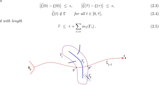
e τ ≤ τ +X i>ν m1(Γi). (2.5) x R 0 ξ j−1 j Γj + P _ Γ γ k P
Figure 3: The construction used in the proof of Lemma3.4. If the trajectoryξj−1(·) crosses the set Γj,
we construct a detourγj of radiusrj around Γj. At a subsequent step, we may be forced to construct a second detour to avoid hitting the component Γk. Hence the new path may get closer to Γj. In the inductive construction, it is essential to show that all paths keep a uniformly positive distance from Γj.
Proof. Let >0 be given. The new path ξewill be obtained as limit of a sequence of paths
ξj : [0, τj]7→ R2, j ≥0, by an inductive procedure. Each inductive step will also determine
two auxiliary constants rj, δj >0.
1. The induction starts by setting τ0 =τ, and defining ξ0(t) =ξ(t) for all t≥0. Moreover,
we chooseδ0 >0 so that
δ0 <
4, δ0 < d(ξ(t),Γi) for all t∈[0, τ], i= 1, . . . , ν. (2.6)
For everyj ≥1, the constantsrj, δj >0 and the pathξj : [0, τj]7→R2 will satisfy the following
properties.
(i) For everyi≤j and t∈[0, τj] one has
d ξj(t),Γi
≥ (2−2i−j)δi. (2.7)
(ii) Forj≤ν we simply take ξj =ξ0. Forj > ν, the length of the pathξj satisfies
(iii) The endpoints satisfy
|ξj(0)−ξ(0)| ≤ (1−2−j), |ξj(τj)−ξ(τ)| ≤ (1−2−j). (2.9)
(iv) The constant rj is chosen so that rj < δj−1/4. Moreover, every component Γk which
intersectsB(Γj,2rj) has lengthm1(Γk)< δj−1/4.
(v) The constantδj ∈]0, rj/4] is chosen so that, for everyk≥1 such that
Γk∩ B(Γj,2rj)\B(Γj, rj/2) 6 = ∅, (2.10) one has 4δj ≤ d(Γk,Γj) = min. n |x−y|; x∈Γj, y∈Γk o . (2.11)
Note that, even if we chooseξj =ξ0 forj = 1, . . . , ν, it is not possible to start the induction
procedure at j = ν. Indeed, the initial steps must be performed in order to define suitable constantsrj, δj,j = 1, . . . , ν.
2. Assuming that the induction has been completed up to step j−1, we describe how to accomplish stepj.
Consider the pathξj−1: [0, τj−1], and the connected component Γj. For a given radius r >0,
define
γj = [boundary of the unbounded connected component of. R2\B(Γj, r)].
This is a simple closed curve, that winds around Γj, and has length ≈2m1(Γj). We choose
r=rj >0 small enough, so that the following holds:
m1(γj) < (2 +)m1(Γj), (2.12) rj < δj−1 2 , rj < 1 4 1min≤i<jd(Γi,Γj), (2.13) and moreover
(Pj) Every connected componentΓk, k6=j, that intersects B(Γj,2rj) has length< δj−1/4.
(P0j) Every disc of radiusδj−1intersects the unbounded connected component ofR2\B(Γj, rj).
Note that all the above can certainly be achieved, because there are only finitely many com-ponents Γkwhose length is > δj−1/4. Choosingrj >0 small enough,γj will not intersect any
of them. Moreover, the inequality (2.12) follows by well known results in geometric measure theory [1,14]. Indeed, since Γj is rectifiable, the neighborhoods of radius r around Γj satisfy
lim r→0 m2 B(Γj, r) 2r = m1(Γj).
Hence the co-area formula yields lim inf r→0 m1 ∂B(Γj, r) ≤ 2m1(Γ). (2.14)
We then choose a constantδj according to (v) above.
Finally, the new path ξj : [0, τj] 7→ R2 is defined as follows. If ξj−1(t) ∈/ B(Γj, rj) for all
t∈[0, τj−1], then there is no need to modify the previous path, and we can simply set
τj = τj−1, ξj(t) =ξj−1(t).
Otherwise, we add a detour so that the new path will remain bounded away from the compo-nent Γj of the barrier. For this purpose, define the times
t− = inf.
t∈[0, τj−1] ; ξj−1(t)∈B(Γj, rj) ,
t+ = sup. t∈[0, τj−1] ; ξj−1(t)∈B(Γj, rj) ,
and the points
P− = ξj−1(t−), P+ = ξi(t+).
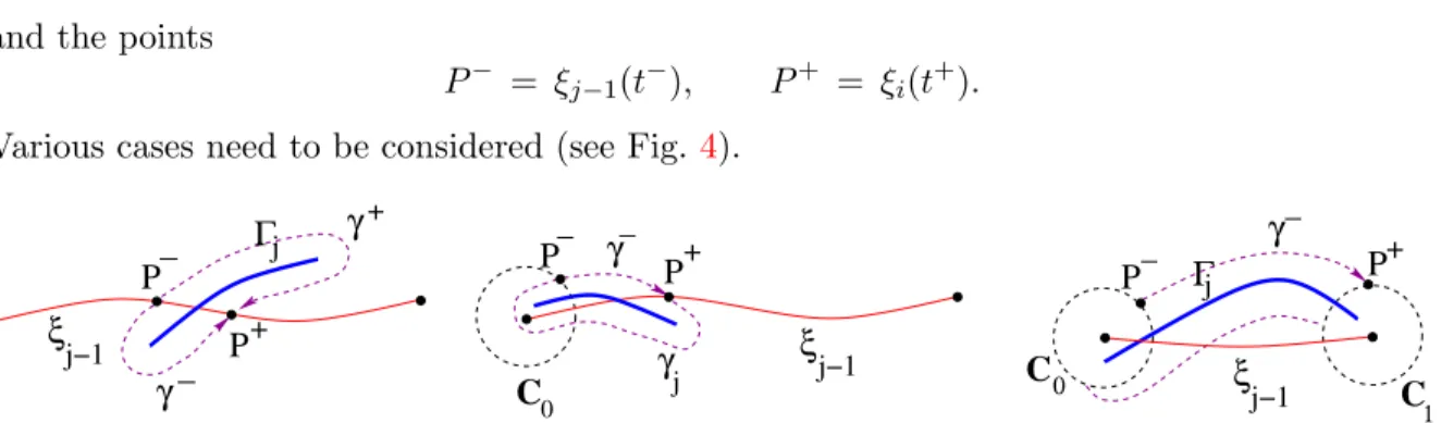
Various cases need to be considered (see Fig.4).
C C 0 γ j C 1 0 Γ γ _ + ξ j−1 j Γ ξ j−1 γ_ P P + P _ _ _ γ P_ P+ P+ ξ j−1 γ j
Figure 4: If the pathξj−1 intersects the component Γj of the barrier, a detour must be constructed.
The figures on the left, center, and right illustrate Cases 1, 2, and 4, respectively.
CASE 1: 0< t−≤t+< τj−1, shown in Fig.4, left.
In this basic case we observe that the two points P−, P+ divide the simple closed curve γj
into two parts, say γj−,γj+. To fix the ideas, assume
sj =. m1(γj−) ≤ m1(γ+j ). (2.15)
Lets7→γj−(s) be an arc-length parameterization of γj−, with γj−(0) = P−, γj−(sj) = P+.
We then define the new path ξj by adding a detour around Γj as follows:
ξj(t) = ξj−1(t) if t∈[0, t−], γj−(t−t−) if t∈[t−, t−+sj], ξj−1(t−sj+t+−t−) if t∈[t−+sj, τj]. (2.16) Here τj = τj−1+sj−(t+−t−). CASE 2: 0 =t−≤t+< τ
CallP+=ξj−1(t+). Observe that, by (2.13) and(P0j), the curveγjhas non-empty intersection
with the circumference
C0=. {y∈R2; |y−ξj−1(0)|=δj−1}. (2.17)
Therefore, starting at P+ and moving along the simple closed curve γ
j, we can reach some
point P− on C0 in two different ways: clockwise and counterclockwise. We chooseγ− ⊂γj
to be the shortest among these two paths.
As shown in Fig.4, center, we parameterize γ− by arc length, so that γ−(0) =P−, γ−(sj) =P+
for somesj >0. Choosing t− so that P− =ξj−1(t−), we define the new pathξj(·) by setting
τj =τj−1−t−+sj and ξj(t) = ( γ−(t) if t∈[0, sj], ξj−1(t+t−−sj) if t∈[sj, τj−1−t−+sj]. (2.18) CASE 3: 0< t−≤t+=τj−1.
In this case, the new pathξj(·) will connect ξj−1(0) with a point on the circumference
C1 =.
y∈R2; |y−ξj−1(τj−1)|=δj−1 . (2.19)
Since this is entirely similar to Case 2, we omit the details. CASE 4: 0 =t−< t+=τj−1, shown in Fig.4, right.
In this case, the simple closed curve γj intersects both circumferences C0 and C1 in (2.17),
(2.19). We then choose a point P− ∈C0 and a pointP+ ∈C1 so that the portion γ− ⊂γj
connecting P− withP+ is as short as possible. We now parameterize γ− by arc length, so that
γ−(0) =P−, γ−(sj) =P+
for somesj >0. The new pathξj(·) is defined simply by setting τj =sj and
ξj(t) = γ−(t) for all t∈[0, sj]. (2.20)
3. Having constructed a sequence of paths ξj : [0, τj] 7→ R2, j ≥ 0, by taking the limit as
j→ ∞ we will obtain a path ξ(e·) which satisfies the properties (2.3)-(2.4), together with e
τ ≤ τ + (1 +)X
i>ν
m1(Γi). (2.21)
For convenience, we extend the definition of each pathξj to all of R+ by setting
Toward a proof of (2.3), we observe that our construction implies |ξj(0)−ξj−1(0) ≤ δj−1 < 2−j . |ξj(τj)−ξj−1(τj−1) ≤ δj−1 < 2−j .
Recalling that ξ0=ξ and summing these inequalities from 1 toj, we obtain (2.9).
4. Our construction guarantees that, for every j ≥ 1, the length τj of the new curve ξj(·)
satisfies (2.8). Notice that, if Case 4 occurs, we have the even sharper bound τj ≤ (1 +)m1(Γj).
In addition, since we are assuming that the initial path ξ(·) does not intersect any of the components Γ1, . . . ,Γν, our choice ofδ0 >0 in (2.6) guarantees that no modification need to
be done in the first ν steps of the algorithm. Hence ξj(·) = ξj−1(·) for all j = 1, . . . , ν. In
particular, this implies
τj = τ for all j= 1, . . . , ν. (2.22)
If one of the Cases 1-2-3 occurs, then our construction yields
ξj(t)−ξj−1(t)| ≤ (1 +)m1(Γj) for all t≥0. (2.23)
In Case 4 the above estimate can fail. However, by (2.9), Case 4 in the above construction can occur only finitely many times. Indeed, there are at most finitely many connected components Γj of length
m1(Γj) ≥ |ξ(τ)−ξ(0)| −4.
We thus conclude that the sequence ξj(·) is Cauchy. As j → ∞, we have the convergence
ξj(t)→ξ∞(t), uniformly fort≥0.
5. Since all pathsξj are Lipschitz continuous with constant 1, the limit pathξ∞is 1-Lipschitz
as well. We can now parameterizeξ∞ by arc-length, and obtain a pathξe: [0, e τ]7→R2, with e τ ≤ lim inf j→∞ τj ≤ τ + (1 +) X j>ν m1(Γj).
Notice that the above estimates follow from (2.22) and (2.8). This proves (2.21). The bounds (2.3) are an immediate consequence of (2.9).
6. In this step we show that (2.4) holds. Namely, the path ξedoes not touch any of the
components Γi,i≥1 of the barrier.
This claim will be proved by showing that, for a fixed j≥1 and every k≥j one has d(ξk(t),Γj) = min.
|ξk(t)−y|; y∈Γj ≥ δj for all t∈[0, τk]. (2.24)
By construction, it immediately follows that
We now observe that, for anyk > j, the pathξk(·) is obtained from ξj(·) by replacing some
of its sections by detours γi−(·), i=j+ 1, . . . , k, where d(γi(s),Γi) = min. n γ(s)−y ; y∈Γi o = ri for alls.
Three cases must be considered.
CASE 1: (2.10) holds, and hence by construction (2.11) holds as well. In this case we have d(γk(s),Γj) ≥ d(Γk,Γj)−d(γk(s),Γk) ≥ 4δj −rk ≥ 3δj.
CASE 2: d(Γk,Γi)>2rj. In this case, for every swe trivially have
d(γk(s),Γj) ≥ d(Γk,Γj)−d(γk(s),Γk) ≥ 2rj−rk > rj ≥ 4δj.
CASE 3: Γk ⊆ B(Γj, rj/2). If ξk(·) =ξk−1(·), the conclusion (2.24) follows by induction on
k. It thus suffices to consider the case whereξk(·) is obtained from ξk−1(·) by inserting some
nontrivial portion of a curveγk⊆ {x; d(x,Γk) =rk}.
In this case, our algorithm implies that there exists a finite sequence j=i(0)< i(1)<· · ·< i(N) =k
such that every curveγi(`) =. {x; d(x,Γk) =rk} intersects the previous one:
γi(`)∩γi(`−1) 6= ∅ for all`= 1, . . . , N.
Considering the diameters of the sets γi(`), we thus have the bound
min s d ξk(s),Γj ≥ min s d γi(1)(s),Γj − N X `=2 diam(γi(`)) ≥ d(Γi(1),Γj)−ri(1) − N X `=2 2ri(`)+m1(Γi(`)) . ≥ 4δj− δj 2 − N X `=2 2·2j−i(`)δj 4 + 2 j−i(`)δj 4 > δj. (2.25)
Indeed, the condition (2.10) applies to Γi(1), hence (2.11) holds. Moreover, using the property
(Pj)with j replaced byi(1), . . . , i(N), we obtain
m1(Γi(`)) ≤
δi(`)−1
4 ≤ 2
j−i(`)δj
4 .
Combining the above three cases, we conclude that (2.24) holds. Taking the limit as k→ ∞, we conclude that d(ξ(t),e Γj)≥δj for allt≥0 and j≥1. This establishes (2.4),
7. To obtain the bound (2.5) on the length of the new path, define
b τ = min. ( e τ , τ+X i>ν m1(Γi) ) .
By (2.21), we trivially have
|τe−τb| ≤ X
i>ν
m1(Γi).
Therefore, if we replace the path ˜ξ by its restriction to the subinterval [0,τb], the conditions
(2.4)-(2.5) are satisfied, while the second inequality in (2.3) will be replaced by
eξ(τb)−ξ(τ) ≤ + X i>ν m1(Γi) ≤ (1 +m1(Γ)).
Since >0 can be chosen arbitrarily small, this completes the proof.
The next result is concerned with the length of the portion of the barrier which is touched by the fire at a given time t. We recall that, if Γ is admissible, the linear bound (1.5) must hold.
Lemma 2.3. Given an admissible barrier Γ, consider the function
ϕ(t) = m1 RΓ(t)∩Γ
. (2.26)
Then
(i) ϕis nondecreasing and right continuous.
(ii) The set of times where the constraint is not saturated U =. n t >0 ; m1 RΓ(t)∩Γ < σt o (2.27) is open.
(iii) The set of times where the constraint is saturated S =. n t≥0 ; m1 RΓ(t)∩Γ = σt o (2.28) is closed.
Proof. 1. For any 0< t1 <2 we have RΓ(t1)⊆RΓ(t2). Hence ϕis nondecreasing.
2. Next, we claim that ϕ it is right continuous. Indeed, consider a decreasing sequence of times tn↓t0. Since the fire propagates with unit speed, we have
RΓ(t n) ⊆ B RΓ(t 0), tn−t0 hence RΓ(t 0)∩Γ = \ n≥1 RΓ(t n)∩Γ .
The right continuity ofϕnow follows from the dominated convergence theorem.
3. By the previous two steps it follows that ϕ is upper semicontinuous. Hence the function t 7→ ϕ(t) −σt is upper semicontinuous as well. We thus conclude that the set U where ϕ(t)−σt <0 is open. The closure ofS =R+\ U follows immediately.
The next lemma will play a key role in the sequel. The intuitive idea is simple: lett=aibe the
first time when the fire front touches the connected component Γi. Immediately afterwards,
the fire starts going around Γi, clockwise as well as counterclockwise, until this connected
component is completely surrounded. This will happen at some timebi withbi−ai≤m1(Γi).
On the other hand, when the fire front does not touch any of the barriers Γj, it expands
freely with unit speed in all directions. Therefore, the distance between level sets of the time functionTΓ increases at unit rate.
Lemma 2.4. Consider a barrier Γ =∪i≥1Γi, written as the union of its compact connected
components. Assume thatR2\Γ is connected.
(i) For each i≥1, the set of times when the fire front touches Γi
Ji =. n t≥0 ; ∂ RΓ(t)∩Γ i 6= ∅ o (2.29)
is contained within an interval [ai, bi] of length bi−ai≤m1(Γi).
(ii) For any 0≤τ < τ0, one has
B RΓ(τ), r ⊆ RΓ(τ0), with r = m 1 [τ, τ 0]\[ i≥1 [ai, bi] . (2.30)
Proof. 1. By the assumptions, each Γi is simply connected. Let
ai = inf. n t≥0 ; RΓ(t)∩Γ i 6=∅ o = min x∈Γi TΓ(x) (2.31)
be the first time when the fire touches Γi. By the lower semicontinuity of TΓ and the
com-pactness of Γi, it is clear that ai is actually a minimum. We will prove part (i) of the lemma
by showing that, at any time τ > ai+m1(Γi), the component Γi is entirely contained in the
interior of the setRΓ(τ).
2. Toward our goal, we first choose ε >0 such that
4ε < τ−ai−m1(Γi), (2.32)
then we choose an integerν > iso large that
X
k>ν
m1(Γk) < ε . (2.33)
Finally, we choose a radius 0< ρ < ε small enough so that
B(Γi, ρ) ∩ Γj = ∅ for all j= 1, . . . , ν, j6=i. (2.34)
With the above choices, we will show that
B(Γi, ρ) ⊂ RΓ(τ). (2.35)
3. To prove (2.35), fix any point x ∈ B(Γi, ρ)\ Γi. For 0 < r < ρ, consider the open
neighborhoodB(Γi, r) of radiusr around Γi. By a suitable choice ofr >0, we claim that the
(i) Callingγ the boundary of the unbounded connected component ofR2\B(Γi, r), we have
m1(γ) < 2m1(Γi) +ε . (2.36)
(ii) The pointx lies in the unbounded connected component of R2\B(Γi, r).
Indeed, the property (i) follows by the same argument used in (2.14). The property (ii) follows from the fact that Γi is compact and simply connected, while x /∈Γi.
x
z
x
y
Γ
i 1 2’
0R
γ
γ
γ
Figure 5: The construction used in the proof of part (i) of Lemma 2.4.
4. As shown in Fig. 5, letx0 ∈Γi be one of the points closest to x, so that|x−x0|< ρ. By
construction, the segment with endpoints x0, xintersects the simple closed curveγ at least at one point, sayy ∈γ. This implies
|x−y| < |x−x0| < ρ ≤ ε. (2.37) Next, since RΓ(a
i)∩Γ 6= ∅, there exists a trajectory for the fire that starts inside R0 and
crosses the curve γ at some pointz before timet=ai.
We now consider the pathξ : [0, `]7→R2 obtained by concatenating the following three paths: • A path γ1, starting inside R0 and reaching z∈ γ without crossing the barrier Γ. This
path has length`1 < ai.
• A pathγ2 contained withinγ, starting at z and ending aty. Since we can move along
γ both clockwise or counterclockwise, by choosing the shorter path we can assume that γ2 has length
`2 ≤
1
2m1(γ) < m1(Γi) +ε.
• A pathγ3 consisting of the segment with endpointsy, x. By (2.37), its length is `3 < ε.
The total length of this pathξ(·) is thus
` = `1+`2+`3 < ai+ m1(Γi) +ε
+ε < τ−2ε.
Notice that, by construction, the path ξ does not cross any of the components Γ1, . . . ,Γν.
Applying Lemma2.2, for any ε0>0 we can find a new path ξe: [0,`]e 7→R2\Γ such that e ξ(0)∈R0, eξ(`)e −x < ε0,
and moreover e ` ≤ ai+m1(Γi) + 2ε+ X k>ν m1(Γk) < τ.
This implies x∈RΓ(τ), as claimed. Hence part (i) of the lemma is proved.
5. It now remains to prove (ii). Without loss of generality, we can assume that the intervals [ai, bi] are labelled according to decreasing length, so that
b1−a1 ≥ b2−a2 ≥ · · · (2.38)
Let 0< τ < τ0 and ε >0 be given. Choose ν >1 large enough so that (2.33) holds. We now express the open set
]τ, τ0[\ [ 1≤i≤ν [ai, bi] = m [ k=1 ]τk, τk0[
as the union of finitely many disjoint open intervals. Next, we choose an integerν0 > ν such that
X
i>ν0
m1(Γi) < ε0 =.
ε
m, (2.39)
and define the times
tk =. τk+ε0, t0k
.
= τk0 −ε0. Finally, for k= 1, . . . , m, we define the sets of integers
Ik =.
n
i; ν+ 1 ≤ i ≤ ν0, [ai, bi]∩]τk, τk0[ 6= ∅
o
. Notice that, by (2.38), these sets are mutually disjoint.
6. Toward a proof of (2.30) we will show that, for every k= 1, . . . , m, one has
B RΓ(tk), rk ⊆ RΓ(τ0 k), with rk = (τk0 −τk)−3ε0− X i∈Ik m1(Γi). (2.40)
Notice that (2.40) implies
B RΓ(τ), r ⊆ RΓ(τ0), (2.41) with r = m X k=1 rk = m X k=1 (τk0 −τk−ε0)−3mε0− m X k=1 X i∈Ik m1(Γi) ≥ m1 [τ, τ0]\ ν [ i=1 [ai, bi] ! −3mε0− X ν<i≤ν0 m1(Γi) ≥ m1 [τ, τ0]\ +∞ [ i=1 [ai, bi] ! −ε−3mε0−ε = m1 [τ, τ0]\ +∞ [ i=1 [ai, bi] ! −5ε. (2.42)
Since hereε >0 can be taken arbitrarily small, this yields (2.30).
7. It thus remains to prove (2.40), for eachk∈ {1, . . . , m}.
Consider any point y∈B(RΓ(tk, rk)) with y /∈RΓ(tk), and choose a pointx0 ∈RΓ(tk) which
minimizes the distance from y. For any given ρ >0, we can then choose a point y0 ∈RΓ(tk)
with|y0−x0|< ρ. Notice that we can also assume
lim h→0+ 1 h2m1 Γ∩B(y0, h) = 0, (2.43)
because this property holds at a.e. point x∈R2, w.r.t. Lebesgue measure.
Call γ the segment with endpoints y0, y, and let ξ : [0, `]7→R2 be an arc-length
parameteri-zation of this segment, oriented fromy0 toy. Notice that this implies ` < rk.
In order to use Lemma2.2, we claim that, among all the connected components Γi, 1≤i≤ν0
the only ones that can have a non-empty intersection with γ are the components Γi, with
i∈Ik. Indeed, consider the set of indices
I− =. i≤ν; [ai, bi]⊆[0, τk] ∪ I1∪ · · · ∪ Ik−1 (2.44)
For everyi∈I−we havebi≤τk< tk. HenceRΓ(tk) contains a neighborhood of Γi. Therefore,
sincey lies outsideRΓ(t
k), a segment of minimum length joining y with a point x0 ∈RΓ(tk)
cannot intersect Γi. The same holds if we choosey0 sufficiently close tox0.
Summarizing the previous discussion, giveny∈B RΓ(tk), rk
\RΓ(t
k), we can findy0∈RΓ(tk)
and a radius ρ >0 small enough such that (i) ` =. |y0−y| < rk.
(ii) The segment γ with endpoints y0, y does not intersect any of the compact connected
components Γi withi∈I−.
(iii) The circumference Σ centered at y0 with radiusρ satisfies
Σ =. {x∈R2; |x−y0|=ρ} ⊂ RΓ(tk)\Γ. (2.45)
Notice that the (2.45) is made possible thanks to (2.43). Next, consider the set of indices
I+ =. i≤ν; ai ≥τk0 ∪ Ik+1 ∪ · · · ∪ Im.
Arguing by contradiction, we show that none of the components Γi with i∈I+ can intersect
the segmentγ. Indeed, if the intersection is nonempty, define ¯
s = min.
s∈[0, `],; ξ(s)∈Γi for some i∈I+ .
For everys <s, an application of Lemma¯ 5.1would imply the existence of a sequence of paths ξj : [0, `j]7→R2\Γ such that
and whose length satisfies lim sup j→∞ `j ≤ s+ X i∈Ik m1(Γi) + X i>ν0 m1(Γi) < rk+ X i∈Ik m1(Γi) +ε0. (2.46)
We now observe that, for alljlarge enough, the pathξj(·) crosses the circumference Σ at some
point ξj(sj). By taking the restriction of ξj to the subinterval [sj, `j], we obtain a sequence
of pathsξej, of length≤`j, where the initial point lies on Σ⊂RΓ(tk) and the terminal points
converge to y. This implies
TΓ(ξ(s)) ≤ tk+ lim inf
j→∞ `j ≤ tk+rk+
X
i∈Ik
m1(Γi) +ε0.
Sincescan be taken arbitrarily close to ¯s, recalling (2.40) we conclude that the pointξ(¯s)∈Γi∗
lies inside the setRΓ(T), with
T = tk+rk+ X i∈Ik m1(Γi) +ε0 = (τk+ε0) + (τk0 −ε0−τk)−3ε0− X i∈Ik m1(Γi) + X i∈Ik m1(Γi) +ε0 < τk0 .
Since i∗ ∈I+, by definition this implies ai∗ ≥τ0
k, reaching a contradiction.
8. In view of the previous step, we can now apply Lemma5.1to each segment with endpoints y0, γ(s), for 0 < s < `=|y−y0|. This yields a sequence of pathsξej : [0, `j]7→R2, joining a
point xj ∈Σ⊂RΓ(tk) with a point yj which becomes arbitrarily close to ξ(s) as j→ ∞. All
these pathsξej do not cross Γ. Their lengths`j satisfy the uniform bound
`j ≤ s+ X i∈Ik+ m1(Γi) +ε0 ≤ rk+ X i∈Ik+ m1(Γi) +ε0 ≤ (τk0 −tk)−ε0.
For every 0≤s < `, this implies
γ(s) ∈ RΓ(τ0
k−ε0) ⊆ RΓ(τ
0
k).
Letting s → `, we obtain γ(s) → y, and hence y ∈ RΓ(τ0
k). This establishes the inclusion
(2.40) for everyk= 1, . . . , m, thus completing the proof.
3
Properties of the minimum time function with obstacles
Assume that the initial setR0 where the fire is burning att= 0 has finite perimeter. Consider
a barrier Γ = ∪iΓi, written as the union of its connected components. For every fixed time
T >0, the truncated function
x 7→ minT , TΓ(x)
has bounded variation. Indeed, as shown in [13], it is an SBV function. By the co-area formula it thus follows Z T 0 m1 ∂RΓ(t)dt < ∞. (3.1)
As a consequence, for a.e. timet∈[0, T], the boundary∂RΓ(t) is a curve with finite length.
We now consider a sequence of barriers Γ(n),n≥1, converging to a barrier Γ, and study the behavior of the corresponding minimum time functionsTΓ(n). Two cases will be studied. The first lemma deals with the case where each barrier has a finite number of connected compo-nents. The second lemma is concerned with barriers having countably many compocompo-nents. For the definition and properties of the Hausdorff distance between compact sets we refer to [2,7].
Lemma 3.1. Let a bounded open set R0⊂R2 be given. Consider a barrierΓ =∪Ni=1Γi which
is the union of finitely many compact, simply connected, rectifiable components. Let Γ(n) =
∪N i=1Γ
(n)
i , with n ≥ 1, be an approximating sequence of barriers. Assume the convergence
w.r.t. the Hausdorff distance:
lim
n→∞ dH(Γ
(n)
i ,Γi) = 0 for each i= 1, . . . , N. (3.2)
(i) For every x∈R2\Γ, one has
TΓ(x) = lim
n→∞ T
Γ(n)
(x). (3.3)
(ii) For eachn≥1, letξn: [0, τn]7→R2 be an optimal trajectory reaching a pointx∈R2\Γ in minimum time without crossing Γ(n). If τn→τ and ξn(·)→ξ(·) uniformly on every
compact subset of [0, τ[, then ξ(·) is an optimal trajectory reaching x in minimum time without crossing Γ.
Proof. 1. Toward a proof of (i), consider a minimizing sequence of 1-Lipschitz paths ξν :
[0, τν]7→R2 , satisfying ξν(0)∈R0, ξν(t)∈/ Γ for allt∈[0, τν], |ξ(τν)−x|< 1 ν , τν → T Γ(x) as ν→ ∞.
Since Γ is compact and by assumption x /∈ Γ, we conclude that, for allν large enough, the segment joining ξ(τν) with x will not touch Γ. By adding this segment to the path ξν we
obtain another sequence of 1-Lipschitz paths ˜ξν : [0,Teν]7→R2\Γ, with
˜
ξν(Teν) =x for all ν , lim
ν→∞Teν = T
Γ(x). (3.4)
By the compactness of the barriers Γ(n), for eachν ≥1 there exist an integernν large enough
such that ˜ξν(t)∈/ Γ(n) for all n≥nν and all t∈[0,Teν]. This immediately implies e
Tν ≥ lim sup n→∞
TΓ(n)(x).
Together with (3.4), this yields
TΓ(x) ≥ lim sup
n→∞ T
Γ(n)
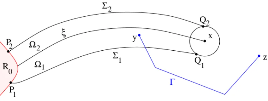
2. To prove (ii) we observe that, by (3.5), τ ≤TΓ(x). It thus only remains to prove that the limit pathξ(·) is admissible. Sincex /∈Γ, there existsρ >0 such thatB(x, ρ)∩Γ =∅. In the following, to simplify notation, we still denote by ξ the set of points {ξ(t) ; t ∈[0, τ]} ⊂ R2.
For a given 0 < r << ρ sufficiently small, consider the neighborhood B(ξ, r), and let Σ be the boundary of the unbounded connected component ofR2\B(ξ, r). This is a simple closed
curve, which we can parameterize by arc-length, oriented counterclockwise.
As shown in Fig. 6, within Σ we distinguish an arc Σ1 connecting a point in P1 ∈ R0 with
a point Q1 ∈B(x, ρ), and an arc Σ2 connecting a pointQ2 ∈B(x, ρ) with a point P2 ∈R0,
moving counterclockwise. we call Ω the open set bounded by Σ. Moreover, we consider theb
open subset
Ω =. Ωb\(R0∪B(x, ρ))
with its open subsets Ω1 ⊂Ω, bounded between Σ1 and ξ, and Ω2 ⊂Ω bounded between ξ
and Σ2.
3. In the following, for simplicity we consider the case where N = 1, so that Γ and all the approximating barriers Γ(n) contain only one component. Since all components are compact and have a positive distance from each other, the general case follows by the same arguments. Fix a point z ∈ Γ, outside the region enclosed by Σ. We claim that, for every y ∈ Ω1∩Γ,
there exists a path γy ⊆Γ connecting y with z, and touching Σ1 without entering Ω2. More
precisely, we claim that there is a map γy : [0,s]¯ 7→Γ such that
γy(0) =y, γy(¯s) =z, γy(s∗) ∈Σ1, where s∗ = inf.
n
s∈[0,¯s] ; γy(s)∈/Ωo.
To prove this claim, we observe that there exist sequences yn, zn ∈ Γ(n), with yn → y and
zn → z. Since Γ(n) is connected, for each n ≥ 1 there is a path γn joining yn with zn, and
remaining inside Γ(n). By possibly selecting a subsequence and relabeling, we obtain a limit
path γ : [0,s]¯ 7→ Γ, joining y with z. If γ(s) ∈ Ω2 for some 0 < s < s∗, then γ crosses the
pathξ. By uniform convergence γn →γ and ξn →ξ, this would imply that everyξn, with n
suitably large, crosses Γ(n), a contradiction.
We observe that, after reaching the boundary Σ1, for s ∈ [s∗,¯s] the path γy can re-enter
inside Ω. However, it cannot cross ξ. Namely, if it enters through Σ1, it must eventually
leave through Σ1. If it enters through Σ2, it must leave through Σ2. Otherwise, being a
limit of paths γn contained in the approximating barriers Γ(n), these paths would cross the
corresponding paths ξn.
4. Within the compact curveξ, fork= 1,2 we define the subset
Vk =.
n
y∈ξ∩Γ ; there is a path inside Γ joiningy withz, exiting through Σk
o
. (3.6) Since Γ is rectifiable and compact, it follows that V1, V2 are both compact. We claim that
they are disjoint. Indeed, assume that y = ξ(s) ∈V1∩V2. Then, inside Ω∩Γ, we can find
a path joining y with a point y1 ∈ Ω1, and another path joining y with a point y2 ∈Ω2. In
turn, by the previous step, there is a pathγy1 joiningy
1 2 1 Q Q 2 P P 1 1 2 x R ξ 0 2 Σ Ω Ω Σ z y Γ
Figure 6: Showing that the limit pathξis admissible.
z. The union of these paths is a multiply connected rectifiable subset of Γ. This yields a contradiction.
5. By the previous step, we can cover the disjoint compact sets V1, V2 ⊂ [0, τ] with finitely
many disjoint intervals, say [aj, bj] and [cj, dj], so that
V1 ⊆ m [ j=1 [aj, bj], V2 ⊆ m [ j=1 [cj, dj].
Define the corresponding portions of curve γ1(j) =.
γ(s) ; s∈[aj, bj] , γ2(j)
.
=
γ(s) ; s∈[cj, dj] .
We claim that, by choosing a radius δ >0 small enough, for every j= 1, . . . , mone has Γ∩B γ1(j), δ∩Ω2 = ∅, Γ∩B γ2(j), δ
∩Ω1 = ∅. (3.7)
Indeed, if no such radius δ >0 exists, we could find a pointy ∈V1 and a sequence of points
yn →y withyn ∈Γ∩Ω2 for alln≥1. By step 3, for each yn there exists a path joining yn
toz, remaining inside Γ\Ω1. By taking a limit, we obtain a path joiningy withz, remaining
inside Γ\Ω1. This would yield y ∈V2, reaching a contradiction because in step 2 we proved
thatV1∩V2=∅.
6. We now describe how to make a small modification of the pathξ, so that it does not touch the barrier Γ. Fixε >0 and consider the finitely many circumferences with radiusε, centered at the points
Aj =ξ(aj), Bj =ξ(bj), Cj =ξ(cj), Dj =ξ(dj).
In addition, for 0< ε0 << ε, call Σ0 the simple closed curve obtained by taking the boundary of the unbounded connected component of R2\B(ξ, ε0). As in step 2, we distinguish a lower
and an upper portion of this boundary, which we call Σ01,Σ02, respectively.
As shown in Fig.7, for eachj = 1, . . . , m, the portion of the path{ξ(s) ; s∈[aj, bj]}between
Aj andBj, is replaced by two arcs of circumferences centered atAj, Bjtogether with a portion
of the curve Σ02. Similarly, the portion of the path {ξ(s) ; s ∈ [cj, dj]} between Cj and Dj,
is replaced by two arcs of circumferences centered at Cj, Dj together with a portion of the
0
x
ξ
R
Γ
1Σ
’
2A
jB
jCj
jD
’
Σ
Figure 7: By modifying the trajectoryξ(·) along the arcs where it touches the barrier Γ, one can show thatξ is admissible.
not intersect Γ. Moreover, lettingε, ε0 →0, we recover the original path ξ in the limit. This shows thatξ(·) is admissible, proving (ii).
8. By (ii) it now follows
TΓ(x) ≤ lim inf
n→∞ T
Γ(n)
(x). Together with (3.5), this yields (3.3), completing the proof.
Remark 3.2. In the above lemma, the assumptions that each Γi is simply connected and
that x /∈ Γ play an essential role. In Figure 8 shows two cases where these assumptions are not satisfied, and the conclusions fail.
Remark 3.3. In (3.6), one can think of V1 is the set of points where the barrier Γ touches
the optimal trajectory ξ on the right, while V2 is the set of points where Γ touches ξ on the
left. Calling ˙ξ(t) = (cosθ,sinθ) ∈ R2 the tangent vector, by construction the map t7→ θ(t)
is non-increasing along each interval [aj, bj], non-decreasing along each interval [cj, dj], and
constant everywhere else.
ξ n ξ Γ(n) Γ x x 0 R Γ Γ(n) R0
Figure 8: Left: an example showing that (3.3) can fail, if the barrier Γ is not simply connected. For eachn≥1, the barrier Γ(n) is the union of three segments, and
R2\Γ(n)is connected. However, the
limit barrier Γ is the boundary of a triangle, which is not simply connected. None of the pointsxin the interior of this triangle can be reached from R0, without crossing Γ. Right: an example showing
that, ifx∈Γ, the inequality (3.3) can fail. Indeed, here TΓ(x)<limn →∞TΓ
(n) (x).
Lemma 3.4. Let a bounded open set R0 ⊂R2 be given. Consider a barrier Γ = ∪∞i=1Γi and
assume that R2\Γ is connected. For eachν ≥1, consider the finite union Γν =∪νi=1Γi. Call
TΓ, TΓν the corresponding minimum time functions.
(i) For every x∈R2 one has
TΓ(x) = lim
ν→∞T
Γν(x). (3.8)
(ii) For eachν≥1, letξν : [0, τν]7→R2 be an optimal trajectory reachingxin minimum time without crossing Γν. If τν → τ and ξν(·) → ξ(·) uniformly on every compact subset of
[0, τ[, thenξ(·)is an optimal trajectory reachingx in minimum time without crossingΓ.
Proof. 1. To prove (3.8), fix x ∈ R2 and, for every ν ≥ 1, call τ
ν =. TΓν(x). Denote by
ζν : [0, τν]→ R2 an optimal trajectory reaching the point x without crossing Γν. According
to Definition2.1, there exists a second path ξν : [0, τν]→R2\Γν such that
ξν(0)∈R0, |ξ(t)−ζ(t) <
1
ν for all t∈[0, τν]. Applying Lemma 2.2, we obtain a further path ˜ξν : [0,eτν]→ R
2, also parameterized by arc
length, such that
˜ ξ(0)∈R0, ξ˜ν(eτν)−x ≤ 2 ν, ˜ ξν(t)∈/Γ for all t∈[0,eτν],
and with length
e
τν < τν+
X
i>ν
m1(Γi).
Therefore (3.8) follows from
lim sup ν→∞ τν ≤ TΓ(x) ≤ lim inf ν→∞ eτν = lim infν→∞ " τν+ X i>ν m1(Γi) # = lim inf ν→∞ τν.
2. To prove part (ii), as usual we assume that all the optimal trajectoriesξν are parameterized
by arc length. By the previous step one has TΓ(x) = lim
ν→∞T
Γν(x) = lim
ν→∞τn = τ .
To achieve the proof it thus suffices to check that the limit trajectoryξ(·) is admissible. Toward this goal, the key tool is again provided by Lemma 2.2. For each ν ≥ 1, using the lemma we obtain a path ˜ξν : [0,eτν]→R
2 such that ˜ ξν(0)∈R0, ξ˜ν(t)∈/ Γ for allt∈[0,τeν], ξ˜ν(τeν)−ξν(τν) ≤ 1 ν, and with length
e
τν ≤ τν+
X
i>ν
Recalling (2.23) in the proof of Lemma2.2, w.l.o.g. we can assume that ξ˜ν(t)−ξν(t) ≤ 1 + 1 ν X i>ν m1(Γi), (3.9)
for all t ≥ 0. It is understood that here ξν and ˜ξν are extended as constant functions, for
t≥τν and t≥eτν, respectively.
By (3.9), as ν → ∞ the sequence of paths ˜ξν(·) converges uniformly to ξ(·). Hence ξ is
admissible.
4
A regularity property of optimal trajectories
Aim of this section is to study a property of the optimal trajectories for the fire, in the presence of barriers. We begin with a few observations.
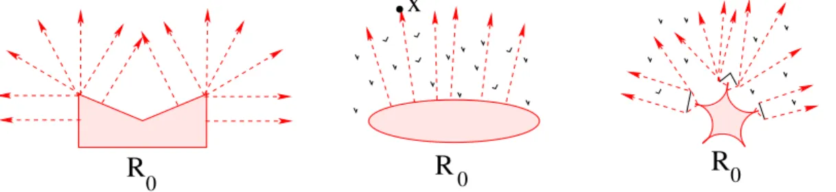
• If no barriers are present, all optimal trajectories are straight lines, and the minimum time function is trivially T(x) =d(x, R0).
• Next, assume that R0 has aC2 boundary. For each point x /∈R0, consider the shortest
segment connecting x with a pointy ∈R0. If the total length of all barriers m1(Γ) = P
im1(Γi)< εis sufficiently small, then most of these segments will not cross Γ. Hence,
as shown in Fig. 9, center, they will yield optimal trajectories for the fire also when barriers are present. Notice that this remains true even if the set Γ of all barriers is dense in R2.
• For a general set R0, however, even if the total length of all barriers is very small, it
can happen that most of the optimal trajectories touch one of the barriers. As shown in Fig.9, this is the case when R0 has cusps, and some of the barriers are placed very
close to these cusps.
R
0R
0R
0x
Figure 9: Left: if no barriers are present, all optimal trajectories are straight lines. Center: if the initial set R0 has smooth boundary and the total length of all barriers is small, then most of the
optimal trajectories do not hit the barrier, and hence are still straight lines. Right: for a general set
R0whose boundary contains cusps, even if the total length of the barriers is small, most of the optimal
trajectories may touch one of the barriers.
Since in general it is not true that most optimal trajectories are straight lines, in this section we prove a somewhat weaker property. Namely: most optimal trajectories contain long straight segments. This property will play a key role in the proof of Theorem 1.5.
Consider again the optimization problem for the fire, in the presence of a barrier Γ. Given an initial set R0, let
R1 =. {x∈R2; d(x, R0)<1} (4.1)
be the neighborhood of radius 1 around R0. For any x ∈ R2, call TΓ(x) the minimum time
needed to reach x from R0 without crossing Γ. Moreover, given an admissible trajectory
t 7→ ξx(t) reaching x in minimum time, we denote by ρ(x) the length of the last portion of this trajectory which is a straight line. More precisely,
ρ(x) = sup. nτ ≥0 ; there exists a trajectoryt7→ξx(t) reachingx in minimum time without crossing Γ, and the velocity ˙ξx is constant on [TΓ(x)−τ, TΓ(x)]o.
(4.2)
Lemma 4.1. Let R0 be a bounded, open set, and call R1 the set in (4.1). Then, for any barrier Γ one has
Z R1 ρ(x)dx ≥ Z R1 d(x, R0)dx− b T2+Tb 2 ·m1(Γ), (4.3) where b T =. sup x∈R1 TΓ(x).
Remark 4.2. In the case where no barriers are present, one has ρ(x) = d(x, R0) and the
bound (4.3) is obvious. We observe that a lower bound on the left hand side of (4.3) cannot be achieved by the trivial estimate
ρ(x) ≥ inf
y∈Γ|y−x|, (4.4)
because the set Γ =∪iΓi can be everywhere dense. In this case the right hand side of (4.4) is
identically zero.
Remark 4.3. Assuming that R2\Γ is connected, so that all barriers are only delaying the
fire, by Lemma 2.2it follows that
b
T ≤ 1 +m1(Γ). (4.5)
4.1 Polygonal barriers.
We shall give a proof of Lemma 4.1 first in a special case where explicit computations can be performed. The general case will then be handled by an approximation argument. In this section, we tassume
(A2) The initial set R0 is the union of finitely many open discs, while the barrier Γ is the union of finitely many (not necessarily disjoint) closed segments.
(i) Every optimal trajectory for the fire, reaching a pointx∈R2 in minimum time without
crossing the barriers, is a polygonal, say with vertices P0, P1, . . . PN. Here P0 ∈ R0,
PN =x, whilePi ∈Γ for all i∈ {1, . . . , N −1}. Indeed, each Pi will be an edge of one
of the segments forming the barrier Γ.
(ii) For every t >0, the boundary of the reachable set∂RΓ(t) is the union of finitely many
arcs of circumferences.
(iii) The set of points which can be reached in minimum time by two distinct trajectories is the union of finitely many segments, or arcs of hyperbolas.
To prove the estimate (4.3) we shall study a family of problems, parameterized by time. Call Γ(t) = Γ∩RΓ(t)
the portion of the walls which are touched by the fire within timet. We obviously have Γ(s) ⊆ Γ(t) for s < t.
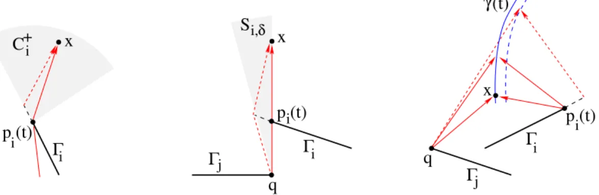
For every t≥0, call ρ(t, x) the function defined at (4.2), but with Γ replaced by the smaller set Γ(t). j γ j (t) i Γ i p (t) q x i Γ q p (t) Γ i i x p (t)i Γ Γ x i δ i, + C S
Figure 10: Left: as the segment Γi becomes longer, the valueρ(x) can decrease at all pointsxin the shaded region. Center: at time increases, the valueρ(x) jumps downward from |x−q|to |x−pi(t)|. Right: the curveγ(t) denotes the set of pointsxreached in minimum time by two distinct trajectories. As time increases, this curve changes in time. At pointsxon this curve, the value ofρjumps upward from|x−pi(t)|to|x−q|.
The estimate (4.3) will be achieved by showing that, for a.e.t∈[0,1],
− d dt Z R1 ρ(t, x)dx ≤ Tb 2+ b T 2 · d dtm1(Γ(t)). (4.6)
To fix the ideas, let Γi(t) ⊆ Γ(t) be one of the segments of the barrier, with an endpoint
pi(t) ∈ ∂RΓ(t) moving along the edge of the advancing fire. For a fixed time t, referring to
the optimization problem with barrier Γ(t), three cases must be considered.
The set of all these points, that we shall call Ωi, is contained within a half discCi, with center
atpi(t) and radius Tb−t. As time increases, for allx∈Ωi we have
d dtρ(t, x) = d dt|pi(t)−x| = ˙ pi(t), pi(t)−x |pi(t)−x| ≥ − p˙i(t) . (4.7)
Observe that the quantity in (4.7) can be negative only on the quarter disc Ci+ =.
x∈Ci; hp˙i(t), pi(t)−xi<0 ,
corresponding to the shaded region in Fig. 10, left. Using (4.7) we compute d dt Z Ωi ρ(t, x)dx ≥ Z Ci+ ˙ pi(t), pi(t)−x |pi(t)−x| dx ≥ − p˙i(t) · Z Tb−t 0 Z π/2 0 cosθ dθ r dr ≥ − Tb 2 2 p˙i(t) . (4.8)
2. Next, we consider points x reached in minimum time by a trajectory whose last portion is a segment with endpoints q and x, and such that pi(t) is a point inside this segment (see
Fig.10, center).
The set of all these points, which we will callDi, is contained on a half line starting atq and
passing throughpi(t), so that
|x−pi(t)| ≤ |x−q| < 1 for allx∈Di.
As time increases, the value of ρ along Di jumps downward from |x−q| to |x−pi(t)|. To
compute the rate of decrease in the integral R ρ(t, x)dx due to such points, fix δ > 0 small and consider the region Di,δ of all points x such that
ρ(t, x) = |x−q|, ρ(t+δ, x) = |x−pi(t+δ)|.
By the triangle inequality one obtains
Z Di,δ ρ(t, x)−ρ(t+δ, x)dx ≤ m2(Di,δ)· pi(t+δ)−q . (4.9)
Observe that Di,δ is contained in a circular sector Si,δ with radius Tb (as the one shaded in
Fig.10, center) whose area can be computed using the vector product
m2(Si,δ) = b T 2 pi(t+δ)−pi(t) × pi(t)−q pi(t)−q +o(δ). (4.10)
Combining (4.9) with (4.10), we conclude
lim δ→0+ 1 δ Z Di,δ ρ(t, x)−ρ(t+δ, x)dx ≤ lim δ→0+ 1 δm2(Si,δ)· |pi(t+δ)−q| ≤ b T 2 p˙i(t) . (4.11)
3. Pointsx on a curveγ(t) reached in minimum time by two distinct optimal trajectories.
As shown in Fig.10, right, we can assume that one of these touchespi(t)∈Γi, while the other
touches some other pointq ∈Γj. These two trajectories have the same length, therefore
|x−q|+TΓ(q) = |x−pi(t)|+TΓ(pi(t)) = |x−pi(t)|+t. (4.12)
Since TΓ(q)≤t, this implies|x−q| ≥ |x−p
i(t)|for all x∈γ(t).
Notice that γ(t) is a branch of hyperbola. For a.e. y∈γ(t) we can choose a neighborhood V of y such that, for everyx∈V, one has
TΓ(t)(x) = min
n
|x−q|+TΓ(q), |x−pi(t)|+t
o
. (4.13)
Assume that, when the barrier is Γ(t), a point x ∈ V is reached in minimum time by a trajectory passing through q, namely
|x−q|+TΓ(q) < |x−pi(t)|+t.
As time increases fromttot+δ and the pointpi(t) is replaced bypi(t+δ), by (4.13) we have
x−pi(t+δ) +TΓ(t+δ)(pi(t+δ)) ≥ x−pi(t+δ) +TΓ(t)(pi(t+δ)) ≥ |x−pi(t)|+t > |x−q|+TΓ(q). (4.14)
According to (4.14), when the barrier increases from Γ(t) to Γ(t+δ), the pointxis still reached in minimum time by a trajectory passing through q. We conclude that, for x∈V,
ρ(t, x) = |x−q| =⇒ ρ(t+δ, x) = |x−q|.
In other words, the functionρ(·, x) cannot have a downward jump. However, it may well jump upward, from|x−pi(t)|to|x−q|.
4. Combining the previous steps1-2-3, for a.e. time t >0 we obtain
d dt Z R1 ρ(t, x)dx ≥ − Tb 2+ b T 2 · X i p˙i(t) = − b T2+Tb 2 · d dtm1(Γ(t)). This proves (4.6).
To achieve the estimate (4.3), we now observe that the integral in (4.6) depends continuously on time, except at finitely many times τk where the topology of Γ(t) changes. To understand
what happens at these exceptional times, as shown in Fig. 11, left, assume that the barrier Γ(t) contains two segments Γ1 and Γ2 with moving endpoints p1(t), p2(t). Assume that, at
timet=τ, the two segments join together: p1(τ) =p2(τ) as in Fig.11, right.
Letx∈R1 and assume that, for t=τ −δ with δ >0 small enough, the pointx is reached in
minimum time by a trajectory passing through p1(t). On the other hand, for t =τ, assume
thatρ(τ, x) = |x−q|, for some pointq along a different optimal trajectory which reaches x without crossing Γ(τ). For t < τ we now have
while at timeτ ρ(τ, x) = |x−q| = TΓ(τ)(x)−TΓ(q). (4.16) Observing that TΓ(τ)(x) ≥ lim t→τ−T Γ(t)(x), TΓ(q) ≤ τ, by (4.15)-(4.16) we conclude ρ(τ, x) ≥ lim t→τ−ρ(t, x). (4.17)
This shows that, at a time τ where the topology of the barrier Γ(·) changes, the function ρ can only have upward jumps.
It remains to observe that, when t= 0, one trivially has Γ(0) =∅and
Z R1 ρ(0, x)dx = Z R1 d(x, R0)dx.
Hence from (4.6) we conclude (4.3).
q q x x Γ(τ) Γ 1 p p 2 Γ 1 2 R0 R0
Figure 11: As time t reaches a critical value τ when two portions of the barrier join together, the topology of Γ(t) changes. Both the minimum timeTΓ(t)(x) and the valueρ(t, x) jump upward.
5. The previous analysis has established the estimate (4.3) in the case where the boundary of R0 is a finite union of circular arcs, and the barrier Γ is the union of finitely many segments.
By an approximation argument, we shall extend the result to a general initial domainR0 and
a general barrier Γ.
As an intermediate step, we show that the estimate (4.3) holds for a general initial set R0,
assuming that Γ has finitely many connected components: Γ = Γ1∪Γ2∪ · · · ∪ΓN.
Indeed, consider a sequence of open sets (R0,n)n≥1 such that:
(i) The boundary of each R0,n is a finite union of circular arcs.
(ii) As n → ∞ the closures of these sets converge in the Hausdorff distance [2], namely dH(R0,n, R0)→0
Moreover, for each k= 1, . . . , N, let (Γk,n)n≥1 be a sequence of compact connected sets such
(iii) Each Γk,n is the union of finitely many segments.
(iv) m1(Γk,n)≤m1(Γk).
(v) As n→ ∞ we have the convergence in the Hausdorff distance: dH(Γk,n,Γk)→0.
For x ∈ R1, let γx,n be a polygonal line reaching x in minimum time. More precisely, γx,n
minimizes m1(γx,n) among all polygonal lines connecting x to some point y ∈ ∂R0 without
crossing the barrier Γn=∪Nk=1Γk,n.
We now observe that, for a.e. pointx∈R1, the functionρ defined at (4.2) satisfies
ρ(x) ≥ lim sup
n→∞
ρn(x). (4.18)
Indeed, we can parameterize every curveγx,n by arc-length, say s7→γx,n(s), with
γx,n(0) = x, γx,n(m1(γx,n)) ∈ ∂R0,n.
By taking a subsequence, we can assume the uniform convergence γx,n →γx on every
subin-terval [0, `] with` < m1(γx). If now the derivatives ˙γx,n are constant over some initial interval
[0,s], the same is true of the derivative ˙¯ γx of the limit functionγx. This proves (4.18).
From the inequality (3.3) in Lemma 3.1it follows
b T =. sup x∈R1 TΓ(x) ≥ lim sup n→∞ b T(n) = lim sup. n→∞ xsup∈R1 TΓ(n)(x).
In turn, since all functions ρn are uniformly bounded, we have
Z R1 ρ(x)dx ≥ lim sup n→∞ Z R1 ρn(x)dx ≥ lim sup n→∞ Z R1 d(x, R0,n)dx− b Tn+Tbn2 2 m1(Γn) ≥ Z R1 d(x, R0)dx− b T +Tb2 2 m1(Γ). (4.19)
6. Finally, we consider the general case where Γ = ∪k≥1Γk is the union of countably many
compact, connected components. We call ρν(·) the map in (4.2), replacing Γ with a finite
union Γν =. ∪νk=1Γk.
Thanks to Lemma3.4, the same argument used to prove (4.18) now yields ρ(x) ≥ lim sup
ν→∞ ρν(x) for a.e. x
∈R1. (4.20)
Moreover, since Γν ⊂Γ for everyν ≥1, we trivially have
b T =. sup x∈R1 TΓ(x) ≥ sup x∈R1 TΓν(x) =. b Tν.
By the previous steps, we already know that the estimate (4.3) holds for everyρν. Taking the
limit asν → ∞and using Lemma 3.4we conclude
Z R1 ρ(x)dx ≥ lim sup ν→∞ Z R1 ρν(x)dx ≥ Z R1 d(x, R0)dx− lim ν→∞ b Tν2+Tbν 2 m1(Γ) ≥ Z R1 d(x, R0)dx− lim ν→∞ b T2+Tb 2 m1(Γ).
This completes the proof of Lemma 4.1.
5
Avoiding barriers more efficiently
As before, we assume that R2\Γ is connected. By the analysis in Lemma 2.2, if p, q /∈ Γ,
then for any ε > 0 we can connect these two points with a path that does not cross Γ and has length ≤ |p−q|+ (1 +ε)m1(Γ). Indeed, one can start with the segment having p, q as
endpoints, and then insert detours to avoid crossing each connected component of Γ.
In this section we prove a sharper result. Namely, if the barrier is sufficiently sparse, we can connect the two points p, q with a path that avoids Γ and has length just slightly larger than |p−q|. We begin by studying the case where Γ is the union of finitely many (possibly intersecting) closed segments, then generalize.
Lemma 5.1. In the t-x plane, consider a barrier Γ consisting of finitely many (possibly intersecting) segments, none of which is parallel to the x-axis. Assume that, for every t >0, the total length of the portion of Γ contained in the strip [0, t]×R satisfies
ψ(t) =. m1
Γ∩([0, t]×R) ≤ √2εt , t∈[0, T], (5.1)
for some0< ε <1. Then there exists a continuous map ξ: [0, T]7→Rwith Lipschitz constant
ε, which satisfies ξ(0) = 0 and whose graph does not cross Γ.
2 2 1 1 a Γ a b Γ 0 t b A(t) x T t ζ t y ζy Γ y
Figure 12: Left: for eacht >0, the setA(t) in (5.2) is the union of finitely many segments [ak(t), bk(t)]. Right: the functionsζ andζy constructed in the proof of Lemma5.3.
Proof. 1. For every t > 0, consider the set A(t) ⊂ R of all values that can be attained by
ε-Lipschitz functions, which are zero at the origin and whose graph does not cross Γ. Namely, as shown in Fig.12), left,
A(t) =. nξ(t) ; ξ is absolutely continuous, ξ(0) = 0,
kξ˙kL∞ ≤ε, (s, ξ(s))∈/Γ for all s∈[0, t] o
.
(5.2)
Since Γ is the union of finitely many segment, we observe that eachA(t) is the union of finitely many intervals, say
A(t) = [
k
At any given time t, we denote by B(t) the set of the endpoints ak, bk which lie along the
barrier Γ, and by F(t) the set of the endpoints which are free, i.e. they do not lie on Γ. The total length of the attainable set A(t) changes at the rate
d dt meas(A(t)) = X k (˙bk(t)−a˙k(t)) ≥ X bk(t)∈F(t) ˙ bk(t)− X ak(t)∈F(t) ˙ ak(t)− X bk(t)∈B(t) |b˙k(t)| − X ak(t)∈B(t) |a˙k(t)|. (5.3) On the other hand, from the definition of ψ at (5.1), it follows
˙ ψ(t) ≥ X ak(t)∈B(t) q 1 + ˙a2 k(t) + X bk(t)∈B(t) q 1 + ˙b2 k(t) ≥ X ak(t)∈B(t) 1 +√|a˙k(t)| 2 + X bk(t)∈B(t) 1 +√|b˙k(t)| 2 . (5.4)
2. To estimate the right hand side of (5.3), consider the function
f(t) = meas(. A(t))−√2(εt−ψ(t)). (5.5)
By (5.1) it follows
meas(A(t)) = f(t) +√2(εt−ψ(t)) ≥ f(t).
Therefore, as long as f(t)>0, we haveA(t)6=∅. In the remainder of the proof we will show thatf is positive and nondecreasing.
To begin, we observe that, fort >0 small, no barriers are present. Hence f(t) = meas(A(t))−√2εt = 2εt−√2εt > 0. Next, using (5.3) and (5.4), from (5.5) we obtain
d dtf(t) = d dtmeas(A(t))− √ 2ε+√2·ψ(t)˙ ≥ #F(t)·ε− X bk(t)∈B(t) |b˙k(t)| − X ak(t)∈B(t) |a˙k(t)| − √ 2ε +√2· X ak(t)∈B(t) 1 +√|a˙k(t)| 2 + X bk(t)∈B(t) 1 +√|b˙k(t)| 2 ≥ #F(t) + #B(t)·ε−√2ε ≥ 2ε−√2ε > 0. (5.6)
Here #F and #Bdenote the cardinality of the sets of free and constrained endpoints, respec-tively. We observe that, as long as A(t) does not vanish, its boundary contains at least two points. This yields the last inequality in (5.6).