RayGUI 2.1
A Graphical User Interface for Interactive Forward and
Inversion Ray-Tracing
U. S. Geological Survey
Open File Report 2004-1426
Authors: Jian-Li Song and Uri ten Brink U.S. Geological Survey, Woods Hole, MA 02543
3
RayGUI 2.1
A Graphical User Interface for Interactive Forward and Inversion
Ray-Tracing for RAYINVR
(U. S. Geological Survey Open File Report 2004 – 1426)
Authors: Jian-Li Song and Uri ten Brink U.S. Geological Survey, Woods Hole, MA 02543
5
Content
1. Introduction to RayGUI 2.1 7
2. Concept of RayGUI 2.1 8
3. Downloading RayGUI 2.1 8
4. Installation of RayGUI 2.1 9
4.1 Installation steps 9
4.2 Set up path and directory setting 10
5. Description of RayGUI 2.1 11
5.1 General description
11
5.2 Menu and Toolbar
13
6. Model 15
6.1 Create a new model 15
6.2 Import model from a text file 16
6.2.1 Import a new model 6.2.2 Import part of a model 6.2.3 Import shots 6.3 Modify model 19
6.3.1 Add/Delete point 6.3.2 Add/Delete layer 6.3.3 Modify location of a point 6.3.4 Modify velocities of a point 6.3.5 Pinch layer 6.3.6 Undo/Redo 7. Travel Time 22
7.1 Travel time window 22
7.2 Observed travel time input file --- tx.in 23
6
8. Running a model
26
8.1 Control parameters 26
8.2 Forward modeling 30
8.3 Inversion 30
9. Zoom and View 30
9.1 Zoom in/out 30
9.2 Drag and zoom on a defined area
31
9.3 View options
31
10. Export 32
10.1 Export PS file 32
10.2 Export XZV velocity model file
32
10.3 Export RMS
32
10.4 Export 1-D profile 33
7
1.
Introduction
RayGUI 2.1 is a graphical user interface of the rayinvr program (Zelt, C.A., and Smith, R.B.,
Geophys. J. Int., 108, 16-34, 1992), a widely-used package for a 2-D forward modeling and inversion of seismic rays in an isotropic medium on UNIX workstations. RayGUI 2.1 is an upgraded version of RayGUI 2.0 (Song, J. L. and ten Brink, U., 2005,Graphical User Interface for Interactive Seismic Ray Tracing Eos,Vol. 86, No. 9, p.90; Song, J. L. and ten Brink, U., 2004, RayGUI 2.0 - A Graphical User Interface for Interactive Forward and Inversion Ray-Tracing, U.S. Geological Survey Open-File Report 2004-1426.). RayGUI 2.1 can be used on computers with either Linux, Unix or MAC-OS X operating systems. The graphical interface greatly facilitates the use of rayinvr, which currently requires text-editing of the velocity model and has a rigid display of model and traveltimes. RayGUI 2.1 enables the user to graphically edit a subsurface velocity model and change the ray-tracing
parameters. The medium consists of distinct layers with velocity values defined at their tops and bases. Velocities can vary laterally along a given layer, and layers can pinch out. Ray-tracing is performed by converting the RayGUI velocity model into rayinvr format and invoking rayinvr from within RayGUI. The modeled rays are plotted in the window of the velocity model. Observed and calculated traveltimes are displayed for comparison to test the velocity model. The display parameters are controlled interactively. The speed has been greatly improved from previous version. The new version no longer has a speed limitation that prevented the user from modeling multiple arrivals from multiple shots. JAVA Jre 1.3 or higher is required to run RayGUI 2.1; FORTRAN 77 and ANSI-C are required to compile
rayinvr and some auxiliary programs. The rayinvr code had to been modified to allow
compilation on Linux and MAC operating systems.
The package is available for non-commercial purposes. Please contact Uri ten Brink at
[email protected] to obtain information on how to download this package. rayinvr, which is part of this package, may not be used commercially. For inquires about rayinvr, please contact Colin Zelt at [email protected].
When you publish papers and reports that include work done with RayGUI 2.1, please cite “Song, J. L. and ten Brink, U., 2004, RayGUI 2.0 - A Graphical User Interface for Interactive Forward and Inversion Ray-Tracing, U.S. Geological Survey Open-File Report 2004-1426.” Please also cite Zelt and Smith (1992).
8
2.
Concept of RayGUI 2.1
RayGUI 2.1 consists of two packages:
• GUI: graphical user interface.
• rayinvr: rayinvr package from Colin Zelt, slightly modified for Linux and MAC operating systems, together with some auxiliary programs.
Philosophy: RayGUI is a Graphical User Interface (GUI) that allows you to interactively edit velocity models and ray-tracing parameters. Ray-tracing is performed by invoking rayinvr from the GUI. After ray-tracing is completed, RayGUI displays observed and modeled traveltimes, and optionally, rays. RayGUI is written in JAVA, rayinvr in FORTRAN77, and auxiliary programs in FORTRAN 77 and ANSI-C.
RayGUI 2.1 uses a Working Directory to support multiple users. The Working Directory is a directory used to store temporary files while RayGUI 2.1 is running. Each user needs to create his/her own working directory to store the temporary files. Indeed, if a user works on more than one project at same time, he/she needs to create a Working Directory for each project. For each project, you need to start RayGUI 2.1 from the Working Directory of this project.
3.
Downloading RayGUI 2.1
Please contact Uri ten Brink at [email protected] to obtain information on how to download RayGUI.
Please inform us at [email protected] after you installed this package let us know on which platform you installed it. This is in your best interest: in order to send you updates bugs files, and information.
Please also inform Colin Zelt ([email protected]), the author of the rayinvr package.
9
4.
Installation of RayGUI 2.1
4.1
Installation steps:
Introduction
Linux Users:
If you are using gcc compiler, make sure g77 is available as a FORTRAN compiler. rayinvr was modified for compiling under Mandrake Linux.
Unix Users:
If you are using SGI or any other system other than Sun Solaris, please pay attention to the Java version. The Java version may not be totally compatible with your system. MAC Users:
MAC users need Fink install and the g77 compiler.
Installation
• Create a new directory for RayGUI, and download RayGUI 2.1 to this directory.
• Unzip and Untar raygui_2.1_for_XXX.tar.gz. This creates the directory rayguidir which contains four sub-directories: bin, raygui, rayinvrpk and example.
bin directory will store the rayinvr executable command;
raygui: RayGUI 2.1 directory, contains all classes of RayGUI2.0;
rayinvrpk: rayinvrpk directory which contains the rayinvr package from Colin Zelt
example: contains an example to run RayGUI 2.1.
• Go to …/rayguidir/rayinvrpk/ rayinvr/ directory and edit Makefile: (… stands for the full path to directory you created for RayGUI 2.1)
In the Makefile under …rayguidir/rayinvrpk/rayinvr/ directory, there are two lines that need to be edited according to the directory rayinvr is located:
EXEDIR=/path_to_rayguidir/bin/
PLTLIB=/path_torayguidir/rayinvrpk/pltlib
10
EXEDIR = …/rayguidir/bin/
Change PLTLIB=/path_to_rayguidir/rayinvr/pltlib into: PLTLIB = …/rayguidir/rayinvrpk/pltlib
These all need to be edited in Makefile. Again, “…” stands for full path to
rayguidir directory
• After editing Makefile, replace the old Makefile with the edited one.
• Remove all *.o files in pltlib directory
• Remove all *.o files in rayinvr directory
• Under …/rayguidir/rayinvrpk/ rayinvr/ directory, type the command make to compile
rayinvr. The executable command of rayinvr will be xrayinvr under “…/rayguidir/bin”.
• Go to …/rayguidir/rayinvrpk/ misc/ directory to compile dmplstsqr. There are four
dmplstsqr versions (dmplstsqr.f, dmplstsqr2.f, dmplstsqr_new.f and dmplstsqr_new2.f)
that you can choice one of them to compile. However, the outfile name has to be
dmplstsqr and need to be put in the …/rayguidir/bin/ directory. Command line examples:
g77 –o …/rayguidir/bin/dmplstsqr dmplstsqr.f // For g77 complier
f77 –o …/rayguidir/bin/dmplstsqr dmplstsqr.f // For f77 complier
4.2
Set up path and directory setting:
• Set up current directory path:
Make sure, JAVA jre 1.3 or higher version is running on your system and paths for Java are set. Include “.” in the PATH environment in your .cshrc file (for Unix and MAC) file or .bashrc file (or .bash_profile)(for Linux). For example, if you have an existing
PATH=/users/username/, change it to PATH = .:/users/username
• Set rayinvr path:
The user needs to make the rayinvr available globally by set up rayinvr path. Add path
“…/rayguidir/bin/xrayinvr” to your path in .cshrc file (for Unix and MAC) or .bashrc file
(or .bash_profile)(for Linux)
• Set RayGUI alias: For single user:
To set alias for RayGUI in your .cshrc file (for Unix and MAC) or .bachrc file (or .bach_profile)(for Linux):
11 for .cshrc file:
alias raygui “cd …/rayguidir/raygui/; java RayGui” for .bashrc
alias raygui = “cd …/rayguidir/raygui/; java RayGui”
The reasons for setting up an alias are: 1. keep command line simple; 2. keep your project directory orgnaized with the temporary files used by RayGUI.
For multiple users:
RayGUI 2.1 supports single user and multiple users. For multiple users, the assumption is that users DO NOT use the same RayGUI working directory. Each user has to create his/her own RayGUI working directory. If a user works on more than one project, he/she needs to create a working directory for each project. A RayGUI working directory is a directory from which the RayGUI is started by the command line “java RayGui” and the temporary files are stored under this directory. For instance, if you have a directory named project1 as your project directory, you need to create another directory, e.g.,
project1_Workingdir, as the RayGUI working directory. When you start to work, go to project1_Workingdir, and start RayGUI from within that directory with the raygui
command. The working directory is not necessary under your project directory. It could be any where you want.
The alias for multiple users is set up differently from above for single user: for .cshrc file:
alias raygui “java -d …/rayguidir/raygui/ RayGui” for .bashrc
alias raygui = “java -d …/rayguidir/raygui/ RayGui”
By setting up the above alias, the user can run RayGUI by simply typing command
raygui. All above, “…” stands for full path to rayguidir directory
5.
Description of RayGUI 2.1
5.1
General description
12
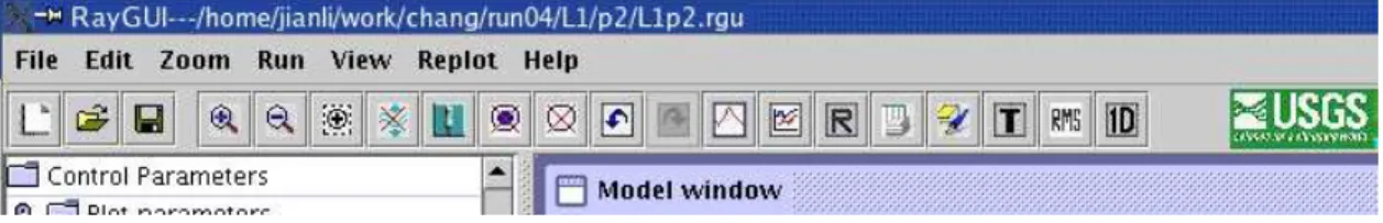
Menu and Toolbar, Control parameter panel, Draw panel and the Curser information panel (Figure 1).
The Menu and Toolbar are located at the top of the window. Most buttons on the toolbar have a corresponding menu item in the submenu of the menu bar, except for delete-layer, add-point, deleted-add-point, go-to-table, and show-time-window buttons.
The Control parameter panel is located on the left side of the window. Click on the button to display the details of each set of parameters.
The Draw panel is on the right side of the window. All the draw functions are completed on this panel. There are two windows available for drawing, one is Model window and another one is Time window. If the Time window is not opened, travel time will be drawn in the Model window together with the model.
The Curser information panel is located at the bottom of the main window which displays the information the curser points to, including current curser screen location in pixels, location x and z values, layer number, upper boundary velocity and lower boundary velocity values. The user can enter the velocity values to update the velocities by pressing the Update velocity button.
13
5.2
Menu and Toolbar
Menu
There are seven menu items on the menu bar: File, Edit, Zoom, Run, View, Replot and Help. Each menu item has several submenu items.
File:
New, creates a new model;
Open, opens an existing model;
Save, saves the current model;
Save as, saves the current model as different name and location;
Import, imports a text model file;
Export PS file, exports current raytrace and travel time as a postscript file;
Export XZV file, exports a text file of X, Z, and V values;
Print, prints the current Draw window (not available currently);
Exit, saves and closes the application.
Edit:
Undo, back to the previous modification;
Redo, redo modification;
Add point, selects the layer to which the point will be added;
Add layer, adds a new layer to the model.
Zoom:
Zoom in, make the model and travel time plots 20% larger;
Zoom out, make the model and travel time plots 20% smaller;
Zoom to original, returns to initial size;
14
Run:
Forward, run forward ray tracing;
Inversion process, run inversion ray tracing or Dmplstsqr (See rayinvr
menu for explanaition).
View:
Show model, model will be shown in the Draw window; Show observed time, observed time will be shown;
Show calculated time, calculated travel time will be shown; Show reduced time, a linearly reduced travel time will be shown; Show rays, rays will be shown;
Show shots, shots will be shown;
Point size, select and change the size of points in the model; Time symbol, draw calculated time as line or as circle.
Replot:
Re-plot the draw without calculation. The user can re-plot the current draw anytime without calculation by pressing R button. If you have the Time window opened, when you change the reduce velocity, you need first press the R button on the Toolbar and then using Draw button on the Time window to re-plot the time.
Help menu will bring up miscellaneous information.
Toolbar
Figure 2 shows the corresponding menu items on the toolbar. The toolbar includes additional functions which are not in the menu. These include Delete layer button, Delete point button, Go to table button, Time window button, RMS button and 1-D profile button.
15
6.
Model
6.1
Create a new model
To create a new model, click on File-New item, a dialog box will pop up. This dialog will ask the user to input the frame parameters for your model, including minimum X, maximum X, minimum Z, maximum Z and the total number of layers in the model (Figure 3).
Figure 3
After filling in the information, press the Ok button. A new table with the information you just entered in above dialog will be brought up (Figure 4). There are six columns in this table: Distance, Upper boundary depth of the layer, Upper boundary velocity of the layer, Lower boundary velocity of the layer, Layer number and Editable. The first row of this table will be the information you entered in the previous dialog. The rest of the rows contain a node of the model. Editable or not corresponds to the values 0 or 1 in the v.in file for each node.
Immediately following the last row of the model parameters, input the shot parameters. Input X, Z values of the shot in the first two columns. Put 0 into the other cells of the shot row.
16
After you finish input the data, press the Save as button. A model will be created and saved as .rgu format and a v.in file will be exported.
Note: the nodes in the table have to be in X order and layer order. For the same layer, the smaller X value node should be first. The layer order has to be in 1,2,3,…
6.2
Import model from a text file
The user can import a model from a text file. Follow the format of the table to create a new model in a text file except for the Editable column. Each point should occupy one row and each row should have six columns:
X, Z, Upper boundary velocity, Lower boundary velocity, layer number
You can use any delimiter between the columns, such as comma, semi colon, space or tab. Again the first row is the model frame information, X-start, X-end, Z-start, Z-end, total layer. Following is the nodes. Shots follow the model nodes and only X, Z values are needed. Bellow is an example of the text file.
0, 100; 0, 50; 2 //X from 0 to 100, Z: 0 to 50, 2 layers 0, 2, 3.2, 4.0, 1 // 1st node of layer 1
10, 1.5, 3.0; 3.8; 1 // 2nd node of layer 1 50; 1.3; 3.5; 4.5; 1 // 3rd node of layer 1 75 2 2.8 3.6 1 // 4th node of layer 1 100 1.7 3.2 4.1 1 // 5th node of layer 1 0, 40, 7.3,7.6,2 // 1st node of layer 2 55, 30, 7.5, 7.7, 2 // 2nd node of layer 2 100, 36, 7.3, 7.6, 2 // 3rd node of layer 2 2, 0.5 // 1st shot
80, 1.0 // 2nd shot 86, 0.6 // 3rd shot
Click on the File-Import, a file dialog will show up. After you select the text file which you want to import, the Load text file window pops up (Figure 5).
17
You have four choices: Load new model, Load model data, Load shots and Load model and shot data.
6.2.1 Import a new model
Load new model option will create a new model using the text file. Press the Next> button to
process to next window to select the format of text file, delimited or fixed width (Figure 6).
Figure 6
Give the start row for the model and the start row for shots and then press the button Next> to select delimiters if you chose Delimited previously (Figure 7).
18
After you select the delimiters, you can press the Preview button to look at the data that will be imported into the model (Figure 8).
Figure 8
You can go through the table to check if there is any error in the model. If there is an error, you can go back a step to correct it. Press Finish button to finish the import and the model will plotted.
Note: Be sure to move the cursor from the last cell you changed to a new cell and click to
choose the new cell before pressing the Finish button, otherwise, the change will not be saved. 6.2.2 Import part of a model
Load model data that option allows user to load part of the model data, such as add layers or
add points to a layer. In this case, you have to open an existing model and your text file contains only layer nodes without the model frame and shots. The operations are similar as Load new model.
6.2.3 Import shots
Load shots that option can add shots to model. The format is same as in the whole model
text file. As described above, an existing model has to be opened before you start to add shots to the model.
Load model and shot data. Use this option if you need to add partial model data and shot
19
6.3
Modify model
The user can add layers to the model, add points to a layer and change X, Z and velocities of a point interactively.
6.3.1 Add/Delete point:
Add points
To add nodes to a layer, go to Edit-Add point and select the layer you want to add points to (Figure 9).
Figure 9
Unlock the Add point button by clicking on it (the cross sign X will disappear when it is unlocked). When Add point button is unlocked, the red-cross disappears. Then you can move the curser to where you want the point added and left click on the mouse button, the node will be added (Figure 10).
Figure 10
To add a point to another layer, change the layer by checking the layer number under Add point submenu of Edit.
Delete point:
20
unlocked), move the curser to the point you want to delete and click on this point, this point will be deleted.
6.3.2 Add/Delete layers
Add a layer
To add a layer, go to the Edit menu and click on Add layer, which brings up the Add layer dialog. You need to give the depth of the layer to be added and select from the following options: Follow higher interface, Follow lower interface, or Straight line interface (Figure 11). The Follow up interface will add a layer which will follow the shape of the layer above it. The velocity values will be copied from the corresponding nodes of the layer above. The user must modify the values of velocities to the new layer.
Figure 11
The Follow lower interface will add a layer which will follow the shape of the layer below it. The velocity values will be copied from the corresponding nodes of the layer below, and user must modify them to the new layer.
The Straight line interface will add a straight interface at the depth you specified. There will be only two nodes at the two ends on this interface. The velocity values are copied from the corresponding nodes in above layer.
Delete layer:
Unlock the Delete layer button by clicking on it (the cross sign will disappear when it is unlocked), then move the curser to any point on the layer that you want to delete, click on the point and this layer will be deleted (Figure 12).
21 6.3.3 Modify location of a point
There are two ways to modify the location of a point. You can drag a point to anywhere within the model to modify its location. Or you can click on the Go to table button to bring up the model table, find the row of the point you want to modify and modify the x and z values. If you use the table to modify a point, you need to save the table and reopen this model.
6.3.4 Modify velocities of a point
The user can modify the velocity by the Update velocity button at the bottom of the window. Move the curser to the point you want to modify, enter the values in the text fields at the bottom of the window and then press the Update velocity button (Figure 13).
Figure 13
The user can press the Go to table button at anytime to bring up the table and modify the model within the table. If you use the table to modify a point, you need to save it and reopen this model.
6.3.5 Pinch layer
There are two steps to completing the pinch layer process.
1. Select the interface to be pinched to: Click on the Pinch layer button or go to Edit-Pinch layer, a dialog will show up and ask you select the interface the layer to be pinched to (See figure 14). The default value is set to Pinch to the upper interface. After you select the interface to be pinch to, press Ok button.
2. Select the distance range to be pinched: When you finish the first step, the cursor will change to an arrow indicating the direction the layer will be pinched to. represents pinch to upper layer and represents pinch to lower interface. Note, on MAC, the cursor status is the same in two cases. Click on a point on the layer where to start to pinch, this point will become red color, then click the point to end the pinch range. This range of the layer will be pinched to the selected interface.
22 6.3.6 Undo/Redo
Undo or Redo action will only take effect on the modifications of model parameters. They will not take effect on the ray draw or time window drawing. The user can undo as many steps as the memory allowed and redo back to the origin.
7.
Travel Time
7.1
Travel time window
The user can split the travel time window from the model window. By pressing the T button on the Toolbar (Figure 15). Initially, the scale in the Time window is same as the scale of Model window horizontal distance and distance range in Time window is same as in the Model window.
23
There are two text fields and five buttons in the Time window. The text fields are the time range (the Y-axis) of the plot. The default start and end range is the full time range of the data. But a narrowed range, and hence, a vertical magnification, can be entered. After entering a new time range, remember to press the Replot button to plot the new travel time range. Within the Time window, the user can zoom in and zoom out the draw scale. Pressing the Original button, the scale will be back to Model window’s scale (Figure 16).
Figure 16
7.2
Observed travel time input file --- tx.in
The observed travel times are still stored in the tx.in file, as rayinvr required. The user must follow the format required by tx.in exactly. Following is an example of tx.in format: shot distance| travel time | uncertainty | phase #
|--- 0 ~ 9 ---|---10 ~ 19 ---|---20 ~ 29 ---|--- 30~39---|
10.000 -1 0.000 0 // shot 1
5.000 0.874 0.050 1 // phase 1 starts 10.000 1.771 0.050 1
……… ………
150.000 26.519 0.050 1 155.000 27.324 0.050 1
15.000 7.413 0.050 2 // phase 2 starts 20.000 7.705 0.050 2
25.000 8.185 0.050 2 ………
………
150.000 26.563 0.050 2 155.000 27.359 0.050 2
24
25.000 9.884 0.050 3 185.000 30.708 0.050 3
……… ………
200.000 32.849 0.050 3 205.000 33.511 0.050 3
90.000 17.485 0.050 4 // phase 4 starts 95.000 18.074 0.050 4
……… ………
300.000 0.300 0.000 0 // shot 2
145.000 27.376 0.050 1 // phase 1 start 150.000 26.503 0.050 1
……… ………
290.000 1 0.050 1 295.000 0.872 0.050 1
145.000 27.463 0.050 2 // phase 2 start 150.000 26.478 0.050 2
………
0.000 0.000 0.000 -1 // end of file
Columns:
0 ~ 9: the shot-receiver offset of receiver
10 ~ 19: travel time observed. For shot, an integer number 1 or -1 to represents the direction that the following travel times are located to shot, 1 to right and -1 to left. 20 ~ 29: travel time uncertainty. For shot, 0.000
30 ~ 39: phase number, it has to be an integer. For shot, 0 Rows:
The first row must be a shot. Following are the phases for this shot. Then, start another shot and its phases. For example,
10.000 -1 0.000 0
or
10.000 1 0.000 0
The second columns indicates the direction of the following travel times located to shot. 1 to right and -1 to left.
Last row of the file has to be:
25
Note: The phase number can be any integer. The user can sign any integer for each phase. However, for one shot, no two phases can have the same number. To facilitate in the inversion, we recommend assigning a number to the observed phase corresponding to the model phase. For example, to the model phase 2.1 (layer 2, refraction, see Figure 19), assign a number 21 to the corresponding observed phase. To model phase 3.2 (layer 3, reflection), assign a number 32 to the corresponding observed phase.
7.3
Observed travel time uncertainty
Observed travel time uncertainties in tx.in file will be used to scale the vertical bar which represents the observed travel time in the plot of travel time. For a larger uncertainty, the travel time vertical bar will be longer. In Figure 17, the uncertainty for three phases are 0.05, 0.10 and 0.15.
26
8.
Running a model
8.1 Control parameters
Plot parameters:
Velocity reduction. There are three options in the velocity reduction, reduce velocity 6,
reduce velocity 8 and user enter reduce velocity. While the Show reduced time in the View menu was checked, the selected reduce velocity will be taken account in drawing (Figure 18).
27 Figure 19
Ray tracing parameters:
Rays. The user can choose the rays to be traced by checking the box corresponding to desired
phases. The user can also define the number of rays to be traced for each phase (Figure 19). The first column, x.1 (x: layer number), is for refraction. The second column, x.2, is for reflection. And the third column 3, x.3, is for head wave. The number of rays to be traced always works for the Forward model option. For inversion, the number of rays always takes the number of observed times. By default, head wave are not selected since they are rarely used.
Shots. The user can choose the shots and the directions to be traced for a shot. Right, left or
28 Figure 20
29
Spacing is the spacing of rays emerging upward for forward modeling. If user enters 0, or
leaves it blank, it will take a default value as (xmax-xmin)/25 (Figure 21). The spacing value only works for head wave.
Inversion parameters:
RayGUI 2.1 will read the tx.in file first before you start the inversion. The arrival types in the tx.in will be shown on this panel (Figure 22).
Ray type, arrivals in the tx.in file. The user can select arrival(s) from this panel for inversion.
In the tx.in file, the user can define the arrival type as he/she wishes, but it has to be an integer.
Uncertainties, the user can define Damping factor, Boundary uncertainty, velocity
uncertainty and travel time uncertainty. These parameters are used for DMPLSTSQR process and is not available at this version
Damping factor is an overall damping factor to control the trade-off between resolution and variance. The default is 1.0.
Boundary uncertainty is the estimated uncertainty of the depth of the boundary nodes (km) written to the file i.out. The default is 0.1.
Velocity uncertainty is the estimated uncertainty of velocities (km/s) written to the file i.out. The default is 0.1.
Time uncertainty is the calculated travel times (s) written to the file tx.out. The default is 0.01.
30
8.2
Forward modeling
When a model is ready, the user can press Forward button on the toolbar or press Forward item under menu Run of the menu bar to run the forward ray tracing (See Figure 23). The user can input the number of rays to be traced for each ray type in the Raytracing parameters panel. If the user does not specify a number, the default number is 10 for each ray type. The larger the number of rays, the longer the time is needed to run the model.
Figure 23
8.3
Inversion
Before starting to run the inversion, the user has to get the observed travel time file tx.in ready. Otherwise the user will be reminded to give the observed time. The inversion parameter panel will show how many observed ray types (phases) you have in the tx.in file. The number next to the checkbox is the number the user defined for that ray type in the tx.in file. In the ray trace parameter selection (Figure 19), user can not select more ray types than observed phases (Figure 22) to run the inversion. For example, suppose you have 5 types of observed phases named 1, 2, 3, 4, and 5, if you want to run inversion for type 2 and 3, you can select only two ray types in the Rays panel under Raytracing parameter. If the selected ray type number in the Rays panel is larger than the number of checked observed ray types (phases), the user will get a warning and the inversion will not run.
For the first time run of dmplstsqr, inversion should be run in advance. Otherwise a warning message will pop up to remind you run inversion first. After each time run of dmplstsqr, inversion will run automatically. This guarantees that dmplstsqr run only one time for an inversion run.
9.
Zoom and View
9.1
Zoom in/out
The user can zoom in or zoom out the plot many times. Each time you zoom in, the scale of plot will enlarge 20% of previous plot, or will shrink by 20% for zoom out. At any zoom
31
scale, the user can go back to original scale (initial scale) by pressing the Zoom to original button. The user can also use the menu item Scale to zoom in or zoom out. Under this option, the scales are 10%, 30%, 50%, 100%, 120%, 150%, 200% and 300% (see Figure 24). The zoom functions under menu bar and tool bar work on both the Model window and the Time window. The Zoom functions in the Time window only work for the Time window.
The zoom in/out functions zoom plots on both dimensions, for the Model window, zoom X and Z dimensions, for the Time window, and zoom X and T dimensions. If the user wants to change the time scale only, he/she can give the time range in the Time window and press the Re-plot button to redraw. The new time range will plot based on your window size.
9.2
Drag and zoom on a defined area.
The user can drag a rectangle in the Model window to zoom in. This rectangle region will be zoomed in to fit the current window size. To do this, the user first left double clicks the
mouse to change the curser into a cross sign, then drags a region. When the mouse is released, the plot will be drawn at the new scale. The distance axis in the Time Window will be
adjusted automatically to correspond to the Model Window. If the user redraws time window in the future, the Time window will take distance range within the rectangle region only to redraw. At any time, the user can press Back to original button to bring the plot back to original scale and the full size.
Fig 24
9.3
View options
There are multiple viewing options: Show model, Show observed time, Show calculated time, Show reduced time, Show rays and Show shots (See Figure 25). The user can select all of them or one of them.
32
There also are two other options: Point size and Time symbol. Point size allows the user to change the size of the plot point in the model. There are four options from 1 - 4. Option 1 is smallest point size and 4 is largest size. The Time symbol option allows user to change the calculated travel time plot symbol. The user can select to draw calculated travel time as a line or as a circle.
Figure 25
10.
Export
This software provides several Export functions for various purposes.
10.1
Export a PostScript file
This function allows the user to export a PS file for current run result. This PS file actually is a copy of PS file from Zelt’s rayinvr package. The PS file will plot travel time and the ray tracing model. The travel time plotted will be at the reduced velocity 8km/s
10.2
Export a XZV velocity model file
This function allows the user to export an xzv velocity model text file. This file will be stored under the current directory by the name “xzv.txt”. The format of the xvz file is “x z v”. Each number is separated by a space.
10.3
Export RMS
Every time when the inversion is completed, the user can press RMS button on the toolbar to show the rms value for the current inversion. When the user presses the RMS button, a dialog box will show up to display the results and ask if the user wants to save the results. The dialog box will display the total number the data used for the inversion and the rms value.
33
10.4
Export 1-D profile
The user can export a 1-D profile of the velocity model using this function. For each 1-D profile, the user has to specify the location where the user wants to take a 1-D profile. When the 1-D profile button is pressed, a dialog will show up and ask the user to input the location for the 1-D profile.
The 1-D profile will be stored under the current project directory and named 1Dxxx.txt, where xxx is the location user input for this 1-D profile. For example, if the user wants to export the 1-D profile at location 126.5km, the 1-D profile will named “1D126.5.txt”
11.
Log
Most information which the rayinvr program outputs should be in the log file, such as forward or inversion result summary, and model error message (Figure 26). The user can press the Log button to show the log information. However, if rayinvr does not end normally, the log information will only show that the rayinvr is aborted. There will be no more
information explaining why the rayinvr failed. In this case, the user can directly run rayinvr under the Working Directory to look at the reason for failure.