Point-by-point reply to final comments by
editor requesting minor changes
GMD-2017-138
C. Lemmen et al.
January 12, 2018
Dear Dr. Valcke,
thank you for your additional efforts to improve our paper. We are very grateful for
your diligent second check of the manuscript and for identifying few remaining issues.
These are now fully addressed in our revision. Please find a point-by-point reply below.
1.
New section 4.4 : Thanks for adding this section but it is quite difficult to follow without an illustration. Please add a Figure sketching the layout of the components on the computing resources used and the coupling interactions between them.Response:
All components in this example run sequentially on the same resources,
thus a sketch of the distribution on compute resources would not help. We made
this clear in the text by adding “This coupled application is to be deployed in
sequential mode on the same set of compute resources for all 13 components”.
Nonetheless we appreciate your confusion (see also your issues below) and agree
to make this point much more clear. We have given special attention throughout
the text for potential pitfalls using the words “shared” and rephrased sentences
that involve sequential/concurrent coupling statements. We also elaborated the
workflow section in several places to explain how this concrete example is related
to the coupling configuration template (Figure 3).
2.
p.6, l.15 to 22 : Thanks for adding this paragraph but I am still not sure which component layout would result from the notation in Fig 3b. As B runs after A and C after B, does it necessarily mean they run sequentially on the same set of computing resources? Or could it be that A and B have each their own set of computing resources, so that A runs for the first coupling period on its resources, then B runs for that first coupling period on its resources with A also running concurrently on its resources for the next coupling period?Response:
We clarified this section and related it better to Figure 3. We also
addressed the confusion between sequential and concurrent coupling. We added
“all components run on shared resources in (default) sequential coupling mode.”
3.
p.6, l.13 : why do you qualify of “sequential” the coupling of Fig 2; in this example the components A, B and C obviously run concurrently.Response:
They
seemingly
run concurrently, but this is an incorrect perspective.
The time axis is in simulation time, and all components share (in “parallel”) the
simulation time. In a wall-clock perspective, they run concurrently. We added the
statement “shown along a simulation time axis, which is independent of the type
of (sequential or concurrent) deployment” in Fig. 2’s caption.
4.
p.17, last paragraph : This assertion on scalability is not meaningful; you have to state that the scalability of MOSSCO applications directly depends on the scalability of the components and on the fact that the coupling workflow does not introduce bottleneck. The statement on the ESMF overhead is OK although a little too qualitative.Response:
We revised the paragraph in multiple places, avoided the confusing
term speedup and provided a percentage ESMF overhead from our scaling
exper-iments.
5.
p.18, first paragraph: the added sentences on speedup are not meaningful either ; this is a speedup with compare to what; it looks like you say that the elapse time is 3000 smaller when running on 192 processors instead of running on 1 processor but I strongly doubt this is the case.Response:
Please see above
6.
p.6, l.7 : I think this sentence is not right ; in Balaji (2016), the atmospheric radiative transfer component has been conFigured to run in parallel with a composite component consisting of ev-ery other atmospheric component, including the atmospheric dynamics and all other atmospheric physics components. , please correct.Response:
We meant the same but you put it better. We now rephrased to “In
their system, an ocean and an atmosphere component run concurrently; within
the atmospheric component, the radiation code is executed concurrently to a
com-posite component containing, in turn, a sequential coupling of all non-radiative
atmospheric processes.”
7.
p.7, last paragraph : What does “scaling” means in this context? Is it just that MOSCCO can couple 0-, 1-, 2-, 3-D models? If so I am not sure that scaling is the right word to use.Response:
We avoided using scaling (or upscaling) in this context as suggested.
We clarified “As a concrete example, the novel Model for Adaptive Ecosystems in
Coastal Seas (MAECS) has been developed iterating between an application for
the lab (zero-dimensional) scale and the three-dimensional regional coastal ocean
scale.”
8.
p.11, l.30 : I would not write identical to the output component because the output component, when used in a parallel model, produces multiple partial files; here the input component will read the different elements in parallel from one global file.Response:
In fact, the input can come from distributed files as well as a global
file. We removed the word parallel to avoid confusion, we rephrased “It inherits
its decomposition from other components in the coupled system. Data can be read
from a single file for the entire domain or from distributed files for all decomposed
compute elements separately. ”
9.
p.13, l.22, I think you cannot write ranging from one-dimensional water-column to three- dimen-sional ... while in your reply to reviewer 2, you write ?There is no coupling between 1D and 3D components in the examples that we currently operate.Response:
We removed the confusing statement and merely talk about
applica-tions at different staapplica-tions, transects, and sea domains.
10.
p.17, l.14&15 : This is misleading ; mediator components will of course have to ensure mass and energy flux when they will include regriddingResponse:
We rephrased the paragraph to address this concern.
11.
p.3, l.1 : for OASIS reference, please use: Craig et al. 2017.p.3, l.2 : for ESMF reference, I think it is better to use : Theurich et al. 2016
Response:
We changed the citations according to the above suggestions
12.
p.3, l.5 : What do you mean by “very differently represented”Response:
rephrased and elaborated as “Their intention is to provide a high-level
user interface and infrastructure for coupling existing and new oceanographic
mod-els whose spatial representation differs greatly, in particular between Lagrangian
and Eulerian representations.”
13.
p.3, l.18 : Given MOSSCO, I think you should not start by Currently, there is no ... ; maybe replace this by something like Up to now, there was no ...p.3, l.29 : This sentence is a bit too heavy, please rephrase it ; I don’t think that the design of a software should emphasize the needs of researchers, instead it should answer them !
Response:
We changed the text accordingly.
14.
p. 5, l.5 : I am not sure coupleability is a real English word ; maybe put this word between quotes, at least the first time it appears in the text.Response:
rephrased as “and provides the basic coupling ability—or “coupleability”—
of the model”
15.
p.5, l.7 : maybe change For the run phase, it is mandatory that this phase refers to for For the run phase, it is mandatory to refer top.5, l.13 : why is operation between brackets ? I think this level of (unclear) detail is not needed here.
Response:
We changed the text accordingly.
16.
p.6, l.15 : I don’t understand what recursive acronym YAML Ain’t Markup Language means.Response:
There’s not much we can do about that. It is meaningless, just like
GNU expands to GNU is Not Unix. We rephrased and added a link: “Users
specify the coupling in a text format using YAML (short for YAML Ain’t Markup
Language, http://yaml.org) notation,”
17.
p.15, l.24 : ... components. In the ... instead of ... components. in the ... p.16, l.17 : Please remove indeed or move it at the beginning of the sentence.p.18, l.6 : This sentence is awkward ; maybe replace it by a simpler sentence like : Multi-component systems may also suffer from low acceptance by the research community.
Response:
We changed the text according to the above suggestions
18.
p.18, l.13 : I am not sure what up-scaling means in this context.Response:
We rephrased: “Yet, it is not clear whether the bottom-up approach
of many interacting modular components leads to an emergent system behaviour
that is desirable and exhibits new insights or whether the system gets tangled up
in coupling complexity.”
19.
p.18, l.24 : benefit from each others? progress ; is the English correct ? Maybe replace by benefit from each other’s progress or benefit from all others’ progress ? p.19, l.33 : please replace OASIS/MCT by OASIS3-MCTResponse:
We changed the text according to the above suggestions
Sincerely
Modular System for Shelves and Coasts (MOSSCO v1.0) – a flexible
and multi-component framework for coupled coastal ocean
ecosystem modelling
Carsten Lemmen
1, Richard Hofmeister
1,4, Knut Klingbeil
2,5, M. Hassan Nasermoaddeli
3,6,
Onur Kerimoglu
1, Hans Burchard
2, Frank Kösters
3, and Kai W. Wirtz
11Institute of Coastal Research, Helmholtz-Zentrum Geesthacht Zentrum für Material- und Küstenforschung,
21502 Geesthacht, Germany
2Department of Physical Oceanography and Instrumentation, Leibniz-Institute for Baltic Sea Research,
18119 Rostock-Warnemünde, Germany
3Section Estuary Systems I, Bundesanstalt für Wasserbau, 22559 Hamburg, Germany
4Institute for Hydrobiology and Fisheries Science, Universität Hamburg, 22767 Hamburg, Germany 5now at Department of Mathematics, University of Hamburg, 20146 Hamburg, Germany
6now at Landesbetrieb Straßen, Brücken und Gewässer, Freie und Hansestadt Hamburg, 20097 Hamburg, Germany Correspondence to:C. Lemmen
Abstract.Shelf and coastal sea processes extend from the atmosphere through the water column and into the sea bed. These processesare driven byreflect::::::::::::intimate::::::::::interactions::::::::betweenphysical, chemical, and biologicalinteractions at local scales, and they are influenced by transport and cross strong spatial gradients. The linkages between domains and many different processes are not adequately described in:::::states::at:::::::multiple::::::scales.::As::a:::::::::::consequence,::::::coastal::::::system::::::::modelling:::::::requires::a::::high
:::
and::::::flexible::::::degree:::of::::::process::::and::::::domain::::::::::integration;::::this:::has::so:::far::::::hardly::::been::::::::achieved::by:current model systems.Their
5
limited integration level in part reflects lackingThe:::::::lack::of:modularity and flexibility; this shortcoming::in::::::::integrated::::::model
hinders the exchange of data and model components and has historically imposed supremacy of specific physical driver models. We here present the Modular System for Shelves and Coasts (MOSSCO, http://www.mossco.de), a novel domain and process coupling system tailored—but not limited—to the coupling challenges of and applications in the coastal ocean. MOSSCO builds on theexisting coupling technologyEarth System Modeling Framework:::::::(ESMF)and on the Framework for Aquatic
10
Biogeochemical Models, thereby(FABM).:::::::::It::::goes:::::::beyond:::::::existing::::::::::technologies:::by:creating a unique level of modularity in both domain and process coupling; the new framework adds rich metadata::::::::including:a:::::clear::::::::separation::of::::::::::component:::and:::::basic :::::
model::::::::interfaces, flexible scheduling, configurations that allow::ofseveral tens of modelsto be coupled, andand::::::::::::facilitation
::
of:::::::iterative::::::::::development::at:::the::::lab,:::the::::::station,::::and:::the::::::coastal:::::ocean:::::scale.:::::::::MOSSCO::is:::rich:::in:::::::metadata::::and::its::::::::concepts:::are
::::::::
applicable::::also::::::outside:::the::::::coastal::::::::domain.:::For::::::coastal:::::::::modelling,::it:::::::contains::::::dozens::of::::::::example:::::::coupling::::::::::::configurations::::and 15
tested setups forcoastalcoupled applications.That wayThus::::, MOSSCO addresses the technology needs of a growing marine coastal Earth System community that encompasses very different disciplines, numerical tools, and research questions.
1 Introduction
Environmental science and management consider ecosystems as their primary subject, i.e. those systems where the organismic world is fundamentally linked to the physical system surrounding it; there exist neither unequivocally defined spatial nor pro-cessual boundaries between the components of an ecosystem (Tansley, 1935). Consequently, holistic approaches to ecological research (Margalef, 1963), to biogeochemistry (Vernadsky, 1998, originally 1926) and to environmental science in general
5
(Lovelock and Margulis, 1974) have been called for.
The need for systems approaches is perhaps most apparent in coastal research. Shelf and coastal seas are described by com-ponents from different spatial domains: atmosphere, ocean, soil; and they are driven by a manifold of interlinked processes: biological, ecological, physical, geomorphological, amongst others. Crossing these domain and process boundaries, the dy-namics of suspended sediment particles (SPM, see Table 2 for abbreviations) and of living particles, or the interaction between
10
water attenuation and phytoplankton growth, for example, are both scientifically challenging and relevant for the ecological state of the coastal system (e.g., Shang et al., 2014; Maerz et al., 2011; Azhikodan and Yokoyama, 2016).
For historical and practical reasons, the representation of the coastal ecosystem in numerical models has been far from holistic. Most often, ecological and biogeochemical processes are described in modules that are tightly coupled to one or a few hydrodynamic models. For example, the Pelagic Interactions Scheme for Carbon and Ecosystem Studies (PISCES, Aumont
15
et al., 2015) has been integrated into the Nucleus for European Modeling of the Ocean (NEMO, Van Pham et al., 2014) and the Regional Ocean Modeling system (ROMS, Jaffrés, 2011). Or, the Biogeochemical Flux Model (BFM) has been integrated in the Massachusetts Institute of Technology Global Circulation Model (MITgcm) (Cossarini et al., 2017) and ROMS. These tight couplings not only exclude important processes at the edges of or beyond the pelagic domain, they also lack flexibility to exchange or to test different process descriptions.
20
To stimulate the development, application and interaction of ecological and biogeochemical models independently of a single host hydrodynamic model, Bruggeman and Bolding (2014) presented the Framework for Aquatic Biogeochemical Models (FABM), which serves as an intermediate layer between the biogeochemical zero-dimensional process models and the three-dimensional geophysical environment models. FABM has been implemented in the Modular Ocean Model (MOM, Bruggeman and Bolding, 2014), NEMO, the Finite Volume Coastal Ocean Model (FVCOM, Cazenave et al., 2016), or the General
25
Estuarine Transport Model (GETM, Kerimoglu et al., 2017). With more than 20 biogeochemical and ecological models included, FABM has enabled marine ecosystem researchers to describe the system’s many aquatic processes.
The process-oriented modularity realized within FABM, however, lacks the means to describe cross-domain linkages. His-torically rooted in atmosphere–ocean circulation models (Manabe, 1969), the coupling of earth domains is the standard concept in Earth System Models (ESM). Domain coupling is also a major challenge in coastal modelling and has been used, for
ex-30
ample, in the Coupled Ocean-Atmosphere-Wave-Sediment Transport (COAWST, Warner et al., 2010) system. COAWST comprises the Regional Ocean Modeling System (ROMS) with a tightly coupled sediment transport model, the Advanced Research Weather Research and Forecasting (WRF) atmospheric model, and the Simulating Waves Nearshore (SWAN) wave model. Each of the components in domain coupling is usually a self-sufficient model that is run in a special “coupled mode”.
Interfacing to other components is done via coupling infrastructure, such as the Flexible Modeling System (FMS, Dunne et al., 2012), the Model Coupling Toolkit (MCT, Warner et al., 2008) and/or the Ocean Atmosphere Sea Ice Soil (OASIS) coupler (Valcke, 2013)(Craig et al., 2017):::::::::::::::, or the Earth System Modeling Framework (ESMF,Hill et al. 2004Theurich et al. 2016::::::::::::::::, see, e.g., Jagers 2010 for an intercomparison of coupling technologies). Recently, Pelupessy et al. (2017) introduced the Oceano-graphic Multipurpose Software Environment (OMUSE) and demonstrated nested ocean and ocean-wave domain couplings.
5
Their intention is to providea:::::::::high-level::::user:::::::interface::::andinfrastructure for couplingvery differently representedexisting and new oceanographic modelswith a high-level user interfacewhose:::::::::::spatial::::::::::::representations:::::differ:::::::greatly,::in::::::::particular::::::::between
:::::::::
Lagrangian:::and::::::::Eulerian:::type:::::::::::::representations. The Community Surface Dynamics Modeling System (CSDMS, Peckham et al., 2013) even allows to couple models implemented in many different languages, as long as all of these describe their capabilities in basic model interface (BMI, Peckham et al., 2013) descriptions. Typically though, only three to five domain components
10
are coupled through one of the above technologies (Alexander and Easterbrook, 2015).
The differentiation between domain and process coupling is not a technical necessity: A typical domain coupling software like ESMF canindeedalso::::be used to couple processes: with the Modeling, Analysis and Prediction Layer (MAPL, Suarez et al., 2007), the Goddard Earth Observing System version 5 (GEOS-5) encompasses 39 process models coupled hierarchically through ESMF; development of these modules, however, is strictly regulated within the developing laboratory. Vice versa, a
15
typical process coupling infrastructure like the Modular Earth Submodel System (MESSy, Jöckel et al., 2005), which initially linked mostly atmospheric processes, has been generalized to support linking at a user-chosen granularity irrespective of the process versus domain dichotomy (e.g., Kerkweg and Jöckel, 2012).
Currently, there isUp::::to:::::now,:::::there:::was:no coastal modelling environment that enables a modular and flexible process (model) integration and cross-domains coupling at the same time, and that is open to a larger community of independent
20
biogeochemical and ecological scientists. The underlying long-term goal for increasingly holistic model systems conflicts with the evolving and diverse research needs of individual scientists or research groups to address very specific problems; it remains difficult to link up-to-date research that is delivered at the (local) process scale to the Earth System scale. Thus we here present the Modular System for Shelves and Coasts (MOSSCO, www.mossco.de), a novelsystem::::::::for:domain and process coupling system:::that::istailored—but not limited—to the coupling challenges of and applications in the coastal ocean. This new system
25
builds on the flexibility of FABM and on the infrastructure provided by ESMF with its cross-domain and many-component hierarchical capability.The coupling philosophy is similar OMUSE and the interoperability follows principles layed out in CSDMS. We here present the major design ideas of MOSSCO and briefly demonstrate its usability in a series of coastal applications.
2 MOSSCO concepts
30
The modularity and coupling concepts proposed in this paperelaborate the design of:::::::describea novel software system that emphasizes::::::::addresses the needs of researchers who want to make maximum use of their existing knowledge in a specific field (e.g., geomorphology or marine ecology) but wish to conduct integrative research in a wider and flexible context. In
strengthening modularitysensuindependence of specific physical drivers, the new concept should, in addition to addressing the problems listed above, support (1) liaisons between traditionally separated modelling communities (e.g., coastal engineers, physical oceanographers and biologists), (2) inter-comparison studies of, e.g., physical, geological, and biological modules, and (3) up-scaling studies where models developed at the laboratory scale in a non-dimensional context are applied to regional, global and Earth System scales.
5
The design of MOSSCO is application-oriented and driven by the demands for enabling and improving integrated regional coastal modelling. It is targeted towards building coupled systems that support decision making for local policies implementing the European Union Water Framework Directive (WFD) and Marine Strategic Planning Directive (MSPD). From a design point of view we envisioned a system that is foremost flexible and equitable.
Flexibility means that the system itself is able to deal on the one hand with a diverse small or large constellation of coupled
10
model components and on the other hand with different orders of magnitude of spatial and temporal resolutions; it is able to deal equally well with zero-, one-, two- and three-dimensional representations of the coastal system. Flexibility implies the capability to encapsulate also existing legacy models to create one or more different “ecosystems” of models. This feature should allow seamless replacement of individual model components, which is an important procedure in the continual development of integrated systems. Flexibly replacing components finally creates a test-bed for model
15
intercomparison studies.
Equitability means that all models in the coupled framework are treated as equally important, and that none is more important than any other. This principle dissolves the primacy of the hydrodynamic or atmospheric models as the central hub in a coupled system. Also, data components are as important as process components or model output; any de facto difference in model importance should be grounded on the research question, and not on technological legacy. As complexity grows
20
by coupling more and more models, this equitability also demands that experts in one particular model can rely on the functionality of other components in the system without having to be an expert in those models, as well.
The equitability design extends to participation: contributions to the development of components or the coupling framework itself is allowed and encouraged. Anyone can use and modify the coupled framework or parts of both in a legal sense by open source licensing, and in an accessibility sense through template codes and extensive documentation.
25
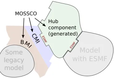
2.1 Wrapping legacy models – first steps inPARSE
As MOSSCO is built around the ESMF hierarchy of components, any existing code that can be wrapped in an ESMF component can be a component in MOSSCO, too. The ESMF user guide (ESMF Joint Specification Team, 2013) suggests a best practice methodPARSEto achieve this componentization of a legacy code.
P repare the user code by splitting it into three phases that initialize, run and finalize a model;
30
R egister the user’s initialize, run, and finalize routines through ESMF;
S chedule data exchange between components;
E xecute a user application by calling it from an ESMF driver.
ThisPARSEconcept allows a smooth transition from a legacy model to an ESMF component. In this concept, the first three steps have to be performed on the model side, and the latter two on the framework side and have been taken care of by the
5
MOSSCO coupling layer. Thepreparationof the code is independent of the use of ESMF and provides the basiccoupleability of:::::::coupling:::::::::ability—or:::::::::::::::::“coupleability”—ofthe model; many existing models already implement this separation into initialize, run, and finalize phases, either structurally, or more formally by implementing a BMI. For the run phase, it is mandatorythat this phase refers toto:::::refer::to:a single model timestep and not to the entire run loop.
Theadaptionof a model’s internal structures to ESMF consists of technically wrapping data into ESMF communication
10
objects, and in providing sufficient metadata for communication. Among these are grid definition and decomposition, units and semantics of data, optimally following a metadata scheme like the widespread Climate and Forecast (CF, Eaton et al., 2011) or the more bottom-up Community Surface Dynamics Modeling System (CSDMS, following a scheme like object +operation ::::::::
operation+ quantity, Peckham 2014). Both are currently being included in the emerging Geoscience Standard Names Ontology (GSN, geoscienceontology.org).
15
ESMF provides the interfaces for models written in either the Fortran or C programming languages; data arrays are bundled together with related metadata in ESMF field objects. All field objects from components are then bundled into exported and imported ESMF state objects to be passed between components. As a third step, the ESMFregistrationfacility needs to be added to a user model; this step is achieved by using template code from any one of the examples or tutorials provided with ESMF. The second and third step (adaptandregister) are typical tasks of what Peckham et al. (2013) refers to as a component
20
model interface (CMI); it is very similar between models (and thus easily accessible from template code) and targets the interface of a specific coupling framework.
MOSSCO contains CMIs for ESMF in all of its provided components (Fig. 1). The current naming scheme follows the CF convention for standard names except for quantities that are not defined by CF; these names (often from biological processes) are modelled onto existing CF standard names as much as possible. MOSSCO also allows the specification within other naming
25
schemes and includes a name matching algorithm to mediate between different schemes. For future development, adoption of the GSN ontology is foreseen.
2.2 Scheduling in a coupled system – the “S” inPARSE
MOSSCO adds onto ESMF a scheduling system (corresponding to the fourth step inPARSE) that calls the different phases of participating coupled models. The coupling time step duration of this new scheduler relies on the ESMF concept of alarms
30
and a user specification of pairwise coupling intervals between models. The scheduler minimizes calls to participating models by flexibly adjusting time step duration to the greatest common denominator of coupling intervals pertinent to each coupled model. Upon reading the user’s coupling specification, (i) models are initialized in random order but with consideration of
special initialization dependencies set by the user; (ii) a list of alarm clocks is generated that considers all pairwise couplings a model is involved in; (iii) special couplers associated with a pairwise coupling are executed; (iv) the scheduler then tells each model to run until that model reaches its next alarm time; (v) advancing of the scheduler to the minimum next alarm time repeats until the end of the simulation.
The MOSSCO scheduler allows for both sequential and for concurrent coupling of model components, or a hybrid coupling
5
mode. In the concurrent mode, components run at the same time on different compute elements::::::::resources; in the sequen-tial mode, components are executed one after anotheron:::::the:::::same:::set::of::::::::compute::::::::resources. Recently, Balaji et al. (2016) demonstrated how a hybrid coupling mode and fine granularity could be used to increase the performance of a system that consists of both highly scalable and less scalable components: In their system,they ran an ocean component concurrently with the radiation code of the atmosphere sequentially to all other atmospheric process components::an::::::ocean:::and:::an::::::::::atmosphere 10
:::::::::
component:::run:::::::::::concurrently;::::::within:::the:::::::::::atmospheric::::::::::component,:::the:::::::radiation:::::code::is:::::::executed:::::::::::concurrently::to::a:::::::::composite
:::::::::
component:::::::::containing:::that:::::::::::encompasses::in::a::::::::sequential::::::::coupling::of::all::::::::::::non-radiative::::::::::atmospheric::::::::processes.
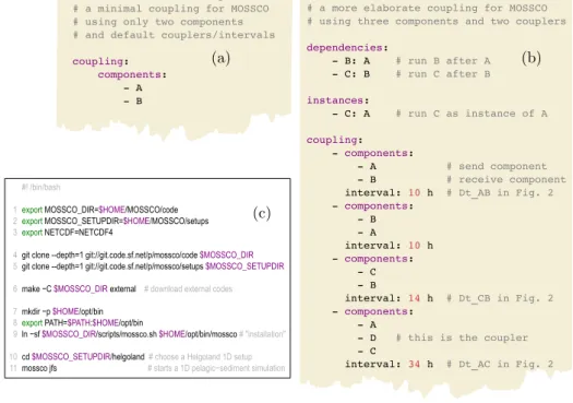
For both concurrent and sequential modes, coupling between components is explicit: the MOSSCO scheduler runs the connectors and mediator components that exchange the data before the components are run. For sequential mode, the coupling configuration allows also a memory efficient scheme where consecutive components operate on shared data that always reflects
15
the most recently calculated data from the previous component (Fig. 2, see also Sect. 3.3.1); such sequential coupling on shared data potentially introduces mass imbalances.
Users specify the coupling in a text format using YAML (recursive acronym::::short:::for:YAML Ain’t Markup Language:, http://yaml.org) notation, a human reader friendly data serialization standard. The itemcouplingcontains a list ofcomponents items that itself contain a list of coupled components; in the simple example (Fig. 3a) two components named “A” and “B”
20
are coupled. By default, these components are coupled in sequential mode with the default connector sharing their data; the execution order of “A” and “B” is not specified. In a more elaborate example (Fig. 3b), the order of components::in:::the::::::::scheduler
is specified in thedependencysection,another instance of “A” with the name::::::::indicating::a:::run::::::::sequence::of::::first::A,::::then:::B,
:::
last::C;:::all::::::::::components:::run::on:::the:::::same:::set::of:::::::compute::::::::resources::in::::::::(default)::::::::sequential::::::::coupling:::::mode.:
:::
The::::::::::::instances::::::section:::::::declares::::that:::the::::::::::component::::::named:“C” is created in the instancessection, and multiple
25
couplings (similar toan:::::::::instance:::(or:::::copy):::of::::“A”;:::this::::::makes::it:::::::possible:::to:::::reuse::::::::::components:::::::multiple:::::times:::in::::::::(possibly
::::::::
different)::::::::::::configurations.::::::::Typically,::::data::::::reader::or::::::writer::::::::::components:::are::::::::::instantiated::::from:a:::::::generic::::::::::input/output::::::::::component ::
to:::::access::::::::different::::files:::for:::::model:::::input:::and::::::output.::::::::Multiple::::::::couplings::::::::between:::the::::three::::::::::components::::“A”,:::::“B”,:::and::::“C”:::are ::::::
present::::with:::::::coupling:::::::::::intervals::::that::::lead::to:::::::::scheduling::of::::::::coupling:::::events:::::::::according::toFig. 2) are provided. Between “A” and “C” a special coupler “D” handles the data exchange instead of the default connector.Coupling time steps are specified as
30
interval.
2.3 Deployment of the coupled system – the “E” inPARSE
MOSSCO provides a Python-based generator that dynamically creates an ESMF driver component in a star topology that then acts as the scheduler for the coupled system. This generator reads the specification of pairwise couplings (Fig. 3) and generates
a Fortran source file that represents the scheduler component. The generator takes care of compilation dependencies of the coupled models, and of coupling dependencies, such as grid inheritance; in addition to the basic init–run–finalize BMI scheme, it also honors multi-phase initialization (as in the National Unified Operational Prediction Capability, NUOPC, ESMF exten-sion) and a restart phase. The generated code structurally and functionally resembles a NUOPC driver, but it does not require implementation of the NUOPC extension, which is currently restricted to handling only structured grid based submodels.
5
A MOSSCO command line utility provides a user-friendly interface to generating the scheduler, (re-)compiling all source codes into an executable and submitting the executable to a multi-processor system, including different high-performance computing (HPC) queueing implementations; this is the fifth step inPARSE. By designing this command line utility and automatic scheduler component creation based on the simple YAML textual coupling specification, MOSSCO provides a fast way to reconfigure, rearrange, extend or reduce coupled systems very quickly, in contrast to more elaborate graphical coupling
10
tools such as the CUPID Eclipse interface (Dunlap, 2013, only for NUOPC).
MOSSCO has been successfully deployed at several national HPC centers, such as the Norddeutsche Verbund für Hoch-und Höchstleistungsrechnen (HLRN), the German Climate Computing Center (DKRZ), or the Jülich Supercomputing Centre (JSC); equally, MOSSCO is currently functioning on a multitude of Linux and macOS laptops, desktops and multiprocessor workstations using the same MOSSCO (bash-based) command line utility on all platforms.
15
The MOSSCO coupling layer is coded in Fortran while most of the supporting structure is coded in Python and partially in Bash shell syntax. The system requirements are a Fortran 2003 compliant compiler, the CMake build system, the Git distributed version control system, Python with YAML support (version 2.6 or greater), a Network Common Data Form (NetCDF, Rew and Davis, 1990) library, and ESMF (version 7 or greater). For parallel applications, a Message Passing library (e.g., OpenMPI) is required. Many HPC centers have toolchains available that already meet all of these requirements. For an individual user
20
installation, all requirements can be taken care of with one of the package managers distributed with the operating system, except for the installation of ESMF, which needs to be manually installed; MOSSCO provides a semiautomated tool for helping in this installation of ESMF. The steps to get MOSSCO running quickly on any suitable computer system are outlined in Fig. 3c. These instructions should get a reader started on carrying out first simulations with a coupled system by typing a dozen lines of code, provided that all requirements are met.
25
3 MOSSCO components and utilities
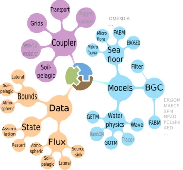
Driven by user needs, MOSSCO currently entails utilities for I/O, an extensive model library, and coupling functionalities (Fig. 4 and Table 1). As a utility layer on top of ESMF, MOSSCO also extends the Application Programming Interface (API) of ESMF by providing convenience methods to facilitate the handling of time, metadata (attributes), configuration, and to unify the provisioning and transfer of scientific data across the coupling framework. The use of this utility layer is not mandatory;
30
any ESMF based component can be coupled to the MOSSCO provided components without using this utility layer.
One of the major design principles of MOSSCO is seamlessscalingdeployment::::::::::from zero-dimensional to three-dimensional spatial representations, while maintaining the coupling configuration to the maximum extent possible. This design principle
builds on the dimensional-independency concept of FABM achieved by local description of processes (often referred to as a box model), where the dimensionality is defined by the hydrodynamic model to which FABM is coupled; MOSSCO generalizes this concept to enable especially the developers of new biological and chemical models to scale up from a box-model (zero-dimensional) to a water-column (one-(zero-dimensional), sediment plate or a vertically resolved transect (two-(zero-dimensional), and a full atmosphere or ocean (three-dimensional) setup. As a concrete example,upscaling ofthe novel Model for Adaptive
Ecosys-5
tems in Coastal Seas (MAECS, Wirtz and Kerimoglu, 2016; Kerimoglu et al., 2017) has been developedin this way going forth and back between the lab:::::::iterating:::::::between::an::::::::::application::for:::the:::lab::::::::::::::::(zero-dimensional)scale and the:::::::::::::::three-dimensional
regional coastal ocean scale.
All utility functions and components, especially the model-independent I/O facilities from MOSSCO, are able to handle data of any spatial dimension. Components that do not define their own spatial representation as a grid or mesh are able to inherit the
10
complete spatial information from a coupled component that provides such a grid: Usually (but not necessarily) biological and chemical models inherit the spatial configuration from a hydrodynamic model; equally well, this information can be obtained from data in standardized grid description formats like Gridspec (Balaji et al., 2007) or the Spherical Coordinate Remapping and Interpolation Package (SCRIP, Jones, 1999). Grid inheritance is specified as a dependency in the coupling specification. 3.1 Model library: Basic Model Interfaces for scientific model components
15
The model library (right branch in Fig. 4) includes new models (e.g., for filter feeders and surface waves) and wrappers to legacy models and frameworks such as FABM or GETM. Some of these wrappers are under development, among them the Hamburg Shelf Ocean Model (HamSOM, Harms, 1997) and a Lagrangian particle tracer model. Here, we briefly document the model collection in particular with respect to their preparation and functioning within the new coupling context.
3.1.1 Pelagic ecosystem component
20
The pelagic ecosystem component (fabm_pelagic_component) collects (mostly biological) process models for aquatic systems. This component makes use of the Framework for Aquatic Biogeochemical Models (Bruggeman and Bolding, 2014). FABM is a coupling layer to a multitude of biogeochemical models which provide the source-minus-sink terms for variables, their vertical local movement (e.g., due to sinking or active mobility), and diagnostic data. Each model variable is equipped with metadata, which is transferred by the ecosystem component into ESMF field names and attributes. Similarly, the forcing
25
required by the biogeochemical models is communicated within the framework and linked to FABM. The pelagic ecosystem component includes a numerical integrator for the boundary fluxes and local state variable dynamics. Advective and diffusive transport are not part of this component but are left to the hydrodynamical model through thetransport_connector (Sect. 3.3.2). The close connection between transport and the pelagic ecosystem requires that the spatial representation of the FABM state variables is inherited from the hydrodynamic model component that performs the transport calculations.
30
Many well known biogeochemical process models have been coded in the FABM standard by various institutes, such as the European Regional Seas Ecosystem Model (ERSEM, Butenschön et al., 2016), ERGOM (Hinners et al., 2015), PCLake (Hu
et al., 2016) and the Bottom RedOx Model (BROM, Yakushev et al., 2017). All pelagic biogeochemical models complying with the FABM standard can equally be used in MOSSCO, while retaining their functionality.
3.1.2 Sediment/soil component
The sediment componentfabm_sediment_componenthosts (mostly biogeochemical) process descriptions for aquatic soils. To allow efficient coupling to a pelagic ecosystem, the sediment component inherits a horizontal grid or mesh from
5
the coupled system and adds its own vertical coordinate, a number of layers of horizontally equal height for the upper soil (typical domain heights range from 10–50cm). State variables within the sediment are defined through the FABM framework
within the 3D grid or mesh in the sediment. As in the pelagic ecosystem component, the state variables, metadata, diagnostics and forcings are communicated via the ESMF framework to the coupled system. The sediment component is the numerical integrator for the tracer dynamics within each sediment column in the horizontal grid or mesh, including diffusive transport,
10
driven by molecular diffusion of the nutrients or bioturbative mixing. Additionally, a 3D variable porosity defines the fraction of pore water as part of the bulk sediment, while all state variables are measured per volume pore water in each cell. FABM’s infrastructure of state variable properties is used to label the new boolean propertyparticulatein FABM models to define whether a state variable belongs to the solid phase within the domain. A typical model used in applications of the sediment component is the biogeochemical model of the Ocean Margin Exchange Experiment OMEXDIA (Soetaert et al., 1996); a
15
version of this model with added phosphorous cycle is contained in the FABM model library as OMEXDIA_P (Hofmeister et al., 2014).
3.1.3 1D Hydrodynamics: General Ocean Turbulence Model (GOTM))
The General Ocean Turbulence Model (GOTM, Burchard et al., 1999, 2006) is a one-dimensional water column model for hy-drodynamic and thermodynamic processes related to vertical mixing. MOSSCO provides a component for GOTM and a
com-20
ponent hierarchy that considers a coupled GOTM with internally coupled FABM within one component (gotm_fabm_component), as many existing available model setups rely on the direct coupling of FABM to GOTM. This way, the modularization—taking a coupled GOTM/FABM apart and recoupling it through the MOSSCO infrastructure, can be verified; the encapsulation of GOTM is implemented in thegotm_component.
3.1.4 3D Hydrodynamics: General Estuarine Transport Model (GETM)
25
MOSSCO provides an interface to the 3D coastal ocean model GETM (Burchard and Bolding, 2002). GETM solves the Navier-Stokes Equations under Boussinesq approximation, optionally including the non-hydrostatic pressure contribution (Klingbeil and Burchard, 2013). A direct interface to GOTM (see Section 3.1.3) provides state-of-the-art turbulence closure in the vertical. GETM supports horizontally curvilinear and vertically adaptive meshes (Hofmeister et al., 2010; Gräwe et al., 2015). The interface to GETM is provided by thegetm_component; any model coupled to GETM via the transport component can
30
topology is made available as an ESMF grid object; typically this grid and subdomain decomposition is communicated to the coupled system where the spatial and parallelization information is inherited by other components.
3.1.5 Model components for erosion, sedimentation, and their biological alteration
The erosion/sedimentation routines of the Deltares Delft3D model (EROSED, van Rijn, 2007) were encapsulated in a MOSSCO component. EROSED uses a Partheniades–Krone equation (Partheniades, 1965) for calculating the net sediment flux of
co-5
hesive sediment at the water–sediment interface for multiple SPM size classes. MOSSCO’s BMI for uses the current version of EROSED maintained by Deltares; it isolates with the help of subsidiary infrastructure the original code from the deeply intertwined dependencies in the Delft3D system. Theerosed_componentcan provide its own spatial representation as a structured grid or unstructured mesh; it can also inherit the spatial information from a coupled component. The functionality of the erosion/sedimentation component is described in more detail by Nasermoaddeli et al. (2014).
10
Flow and sediment transport can be affected by the presence of benthic organisms in many ways. Protrusion of benthic animals and macrophytes in the boundary layer changes the bed roughness and thus the bed shear stress and consequently the sediment transport. The erodibility of sediment can be modified by the mucus produced by benthic organisms; the erodi-bility of the upper bed sediment can be altered by bioturbation generated by macrofauna (de Deckere et al., 2001). In the benthos_component, these biological effects of microphytobenthos and of benthic macrofauna on sediment erodibility
15
and critical bed shear stress are parameterized and provided to other coupled components (e.g. the erosion/sedimentation component) as additional erodibility and critical shear stress factors. The benthos effect model is described in detail by Naser-moaddeli et al. (2017).
3.1.6 Filter feeding model
Thefiltration_componentdescribes the instantaneous filtration by suspension feeders within the water column. This
20
biological filtration model follows Bayne et al. (1993) and describes the filtration rate as a function of food supply; it can be adapted to different species of filter feeders and was recently applied to describing the ecosystem effect of blue mussels on offshore wind farms as thefiltration_componentof MOSSCO (Slavik et al., “The large scale impact of offshore windfarm structures on pelagic primary production in the southern North Sea”, manuscript submitted to Hydrobiologia). The filtration model uses an arbitrary chemical species or compound, say phytoplankton carbon as the “currency” for processing.
25
The amount of ambient phytoplankton carbon concentration is sensed by the model organisms and it is filtered along with the other nutrients (in stoichiometric proportion) out of the environment, creating a sink term for subsequent numerical integration in the pelagic ecological model.
3.1.7 Wind waves
A simple wind wave model is part of the MOSSCO suite. Based on the parameterization by Breugem and Holthuijsen 2007,
30
wave data enable the inclusion of wave effects especially for idealized 1D water column studies, e.g. the consideration of erosion processes due to induced bottom stresses. Coupling to 3D ocean models and the calculation of additional wave-induced momentum forces there, following either the Radiation stress or Vortex Force formulation (Moghimi et al., 2013), is possible as well. For the inclusion of wave–wave or wave–current interaction in realistic 3D applications, the coupling to a more advanced third generation wind wave model like SWAN, WaveWatch III or Wave Atmospheric Model (WAM) would be
5
necessary.
3.2 Input/Output utilities
The input and output (I/O) utilities include general purpose coupling functionalities that deal with boundary conditions, provide a restart facility, add surface, lateral and point source fluxes (lower left branch in Fig. 4).
3.2.1 NetCDF output
10
This component of MOSSCO provides an output facilitynetcdf_componentfor any data that is communicated in the coupling framework. The component writes one- to three-dimensional time sliced data into a NetCDF (Rew and Davis, 1990) file and adds metadata on the simulation to this output. Multiple instances of this component can be used within a simulation, such that output of different variables, differently processed data, and output at various output time steps can be recorded. The output component is fully parallelized with a grid decomposition inherited from one of the coupled science or data components.
15
In order to reduce interprocess communication during runtime, each write process considers only the part of the data (its data tile) that resides within its compute domain. This comes at a cost to the user, who has to postprocess the output tiles to combine for later analysis; a python script is provided with MOSSCO that takes care of joining tiled files.
The output component also adds metadata that is collected from the system and the user environment at the creation time of the output files. Diagnostics about the processing element and run time between output steps are recorded. The structure of the
20
NetCDF output follows the Climate and Forecast (CF, Eaton et al., 2011) convention for physical variables, geolocation, units, dimensions and methods modifying variables. When (mostly biological) terms are not available in the controlled vocabulary of CF, names are built to resemble those contained in the standard.
3.2.2 NetCDF input
Thenetcdf_input_componentof MOSSCO reads from NetCDF files and provides the file content wrapped in ESMF
25
data structures (fields) to the coupling framework. Itis parallelized identical to the output component, andinherits its decom-position from other components in the coupled system. Data can be read::::from::a:::::single:::file:for the entire domain orfrom::::
:::::::::
distributed::::files for all decomposed compute elements separately. Upon reading of data, fields can be renamed and filtered before they are passed on to the coupled system.
The input component is typically used to initialize other components, for restarting, to provide boundary conditions, and
30
with nearest, most recent, and linear interpolation. It also supports reading climatological data and translates the climatological timestamp to a simulation present time stamp in the coupling framework.
3.3 MOSSCO connectors and mediators
Information in the form of ESMF states that contain the output fields of every component are communicated to the ESMF driver; requests for data by every component are also communicated to the ESMF driver component. MOSSCO connectors
5
are separate components that link output and requested fields between pairwise coupled components. MOSSCO informally distinguishes between connector components that do not manipulate the field data on transfer at all (or only slightly), and mediator components that extract and compute new data out of the input data.
3.3.1 Link, copy and nudge connectors
The simplest and default connecting action between components is to share a reference (i.e. a link) to a single field that resides
10
in memory and can be manipulated by each component; in contrast, thecopy_connectorduplicates a field at coupling time. The consideration of a link or copy connector is important for managing the data flow sequence in a coupled system: the copy mechanism ensures that two coupled components work on the same lagged state of data, whereas the link mechanism ensures that each component works on the most recent data available.
Thenudge_connectoris used to consolidate output from two components by weighted averaging of the connected
15
fields. It is typically used as a simple assimilation tool to drive model states towards observed states, or to impose boundary conditions.
These connectors can only be applied between components that run on the same grid (but maybe with a different subdomain decomposition). Thelink_connectorcan only be applied between components with an identical subdomain decompo-sition so that the components have access to the same memory. Components on different grids require regridding, which is
20
currently under development in MOSSCO. 3.3.2 Transport connector
A model component qualifies as a transport component when it offers to transport an arbitrary number of tracers in its numerical grid; this facility is present, for example, in the currentgotm_componentandgetm_component. Thetransport_connector collects state variables to be transported from any coupled component and communicates this collection to the hydrodynamic
25
component based on the availability of both, the tracer concentrations as well as their rate of vertical movement independent of the water currents. This connector is usually called only once per coupled pair of components during the initialization phase. 3.3.3 Mediators for soil–pelagic coupling
One aspect of the generalized coupling infrastructure in MOSSCO is the use of connecting components that mediate between technically or scientifically incompatible data field collections. The soil–pelagic coupling of biogeochemical model
nents with a variety of different state variables raises the need for these mediators. The use of mediators leaves the level of data aggregation and dis-aggregation, and unit conversion to the coupling routine, instead of requiring specific output from a model component depending on its coupling partner component.
For soil–pelagic (or benthic–pelagic) coupling, thesoil_pelagic_connectormediates the soil biogeochemistry out-put towards the pelagic ecosystem inout-put and thepelagic_soil_connectormediates the pelagic ecosystem output
to-5
wards the soil biogeochemistry input, e.g.: (i) dis-aggregation of dissolved inorganic nitrogen to dissolved ammonium and dissolved nitrate (ii) filling missing pelagic state fields for phosphate using the Redfield-equivalent for dissolved inorganic nitrogen (iii) calculation of the vertical flux of particulate organic matter (POM) from the water column into the sediment depending on POM concentrations in the near-bottom water, its sinking velocity and a sedimentation efficiency depending on the near-bottom turbulence. The effective vertical flux is communicated into the pelagic ecosystem component to budget the
10
respective loss, and is communicated to the soil biogeochemistry component to account for the respective new mass of POM. The mediator also handles (iv) dis-aggregation of a single oxygen concentration (allowing positive and negative values) into dissolved oxygen concentration, if positive, and dissolved reduced substances, if negative. (v) aggregation of pelagic POM composition (variable nitrogen to carbon ratio) into fixed stoichiometry POM pools in the soil biogeochemistry.
4 Selected applications as feasibility tests and use cases
15
MOSSCO was designed for enhancing flexibility and equitability in environmental data and model coupling. These design goals have been helpful in generating new integrated models for coastal researchranging from one-dimensional water- column to three-dimensional,with applications at different marine stations (1D),::::::::::::transects::::(2D),transects, and sea domains::::(3D). Below, we describe from a user perspective the added value and success of the design goals obtained from using MOSSCO in selected applications; here, the focus is not on the scientific outcome of the application (these are described elsewhere by, e.g.,
20
Nasermoaddeli et al. 2017, Slavik et al. (subm.),Wirtz and Kerimoglu 2016,and Kerimoglu et al. 2017). All setups described in the use cases are available as open source (with limited forcing data due to space and bandwidth constraints).
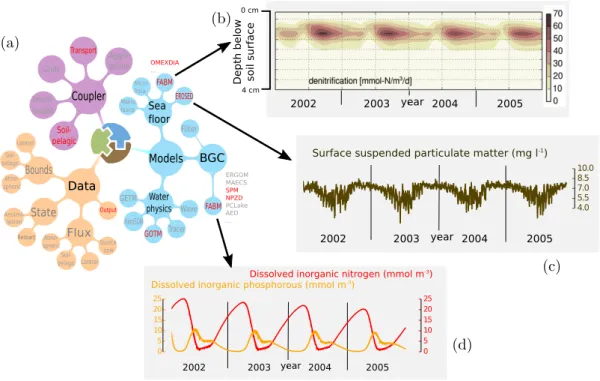
4.1 Helgoland station
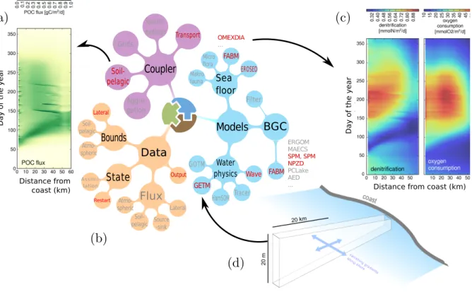
The seasonal dynamics of nutrients and turbidity emerges from the interaction of physical, ecological and biogeochemical processes in the water column and the underlying sea floor. We resolve these dynamics in a coupled application for a 1D vertical
25
water column for a station near the German offshore island Helgoland. Average water depth around the island is 25 m; tidal currents are affected by the M2 and S2 tides with a characteristic spring–neap cycle, with current velocity not exceeding 1 m s−1.
The Helgoland 1D application is realized by a coupled system consisting of GOTM hydrodynamics, the pelagic FABM component with a nutrient–phytoplankton–zooplankton–detritus (NPZD) ecosystem model (Burchard et al., 2005) and two
30
early diagenesis submodel, and coupler components for soil–pelagic, pelagic–soil and tracer transport. This system and setup is described in more detail by Hofmeister et al. (2014).
Simulations with this application show a prevailing seasonal cycle in the model states (Fig. 5). Dissolved nutrients (referred as dissolved inorganic nitrogen) are taken up by phytoplankton, which fills the pool of particulate organic nitrogen during the spring bloom (Fig. 5d). The particulate organic matter sinks into the sediments, where it is remineralized along axis,
sub-5
oxic and anoxic pathways; denitrification, for example, shows a peak in late summer (Fig. 5b). At the end of a year, nutrient concentrations are high in the sediment and diffuse back into the water column up to winter values of 20–25 mmol m−3. The seasonal variation of turbidity is a result of higher erosion in winter and reduced vertical transport in summer (Fig. 5c). 4.2 Idealized coastal 2D transect
The coastal nitrogen cycle is resolved in an idealized coupled system for a tidal shallow sea. This two-dimensional setup
10
represents a vertically resolved cross-shore transect of 60 km length and 5–20 m water depth and has been used by Hofmeis-ter et al. (2017) to simulate sustained horizontal nutrient gradients by particulate matHofmeis-ter transport towards the coast. Within the MOSSCO coupling framework, the 2D transect scenario additionally provides insights into horizontal variability of ero-sion/sedimentation and benthic biogeochemistry. Its coupling configuration builds on the one used for the 1D station Helgoland (Sect.Section::::::4.1); the water-column hydrodynamic model GOTM, however, is replaced by the 3D model GETM; a local wave
15
component and data components for open boundaries and restart has been added.
FigureFig.:::6 shows exchange fluxes between the water column and the sediment for one year of simulation. The simulation of turbidity, as a result of pelagic SPM transport and resuspension by currents and wave stress, provides the light climate for the pelagic ecosystem. The flux of particulate organic carbon (POC) into the sediment reflects bloom events in summer during calm weather conditions. Macrobenthic activity in the sea floor brings fresh organic matter into the deeper sub-oxic layers
20
of the sediment, where denitrification removes nitrogen from the pool of dissolved nutrients. The coupled simulation reveals decoupled signals of benthic respiration, denitrification and nutrient reflux into the water column, which is not resolved in monolithically coded regional ecosystem models of the North Sea (Lorkowski et al., 2012; Daewel and Schrum, 2013). 4.3 Southern North Sea bivalve ecosystem applications
A Southern North Sea (SNS) domain was used in two studies concerning the effects of bivalves on the pelagic ecosystem.
25
Slavik et al. (subm.) investigated how the accumulation of epifauna on wind turbine structures (Fig. 7d) impacts pelagic primary production and ecosystem functioning in the SNS at larger spatial scales. This study is the first of its kind that extrapolates ecosystem impacts of anthropogenic offshore wind farm structures from a local to a regional sea scale. The authors use a MOSSCO coupled system consisting of the hydrodynamic model GETM, the ecosystem model MAECS as described by Kerimoglu et al. (2017), the transport connector, the filter feeder component, and several input and output components (Fig. 7e).
30
They assess the impact of anthropogenically enhanced filtration from blue mussel (Mytilus edulis) settlement on offshore wind farms that are planned to meet the 40-fold increase in offshore wind electricity in the European Union until 2030; they find a
small but non-negligible large-scale effect in both phytoplankton stock and primary production, which possibly contributes to better water clarity (Fig. 7f).
Biological activities of macrofauna on the sea floor mediate suspended sediment dynamics, at least locally. In the study by Nasermoaddeli et al. (2017), the large-scale biological contribution of benthic macrofauna, represented by the key species Fabulina fabula(Fig. 7a), to suspension of sediment was investigated. Simulation results for a typical winter month revealed
5
that SPM is increased not only locally but beyond the mussel inhabited zones. This effect is not limited to the near-bed water layers but can be observed throughout the entire water column, especially during storm events (Fig. 7c). In this coupled application, the hydrodynamic model GETM, the pelagic ecosystem component with three SPM size classes, the erosion– sedimentation and benthic mediation components, several input and one output components, and the transport connector were used (Fig. 7d).
10
4.4 Exemplary workflow
For the SPM bivalve example above (Nasermoaddeli et al. 2017 and Fig. 7c), the coupled system contains 13:modular components: the hydrodynamicgetm_componentandsimplewave_component, a pelagicfabm_component, the benthic erosion/sedimentationerosed_component andbenthos_component, four input and one output component, and the default link_connector, the nudge_connectoras well as thetransport_connector.::::Each:::of:::::these 15
::
13::::::::::components:::is:::::::involved:::in::at::::least::::one:::::::pairwise::::::::coupling:::::::::described::in::a:::::::::::couplings::::::section::of:::the:::::::YAML::::::::coupling
:::::::::::
configuration::::(Fig.::::3b).::::This:::::::coupled:::::::::application::is::to:::be::::::::deployed::in:::::::::sequential:::::mode::on:::the:::::same:::set::of::::::::compute::::::::resources
::
for:::all::13:::::::::::components.
The coupling specification prescribes that grids of the ::::::::horizontal::::::spatial::::::::::::representation::::and:::::::domain::::::::::::decomposition::::are :::::::
provided:::by:::the::::grid::::that::is::::::created::in:::the:::::::::::::hydrodynamic:::::model::::and::::that::is::::::::::::communicated::to:::the:wave, pelagic ecosystem,
20
benthic and input componentsare all inherited from the hydrodynamic component; it also creates four:;:::this::is::::::::achieved:::by
::::::::
specifying:::the::::::::::::hydrodynamic::::::model::as:a::::::::::dependency::of:::::these::::::::::components:(:::::::::::::::dependencies::in:::Fig.::::3b)::::Fourinstances of the netcdf_input_component, for::::(see::::3.2.2:::and::::::::::::instances::in:::Fig.:::3b):::are::::::created::to:::::::providemacrofauna forcing, lateral open ocean boundariesand rivers , as well as restarting,:::::rivers::::::fluxes,::::and:::::restart::::::::::information::::from:::::::netCDF::::files. In the::::first::of
:::
twoinitialization phases, the output components and the hydrodynamic component are initialized first,the latter communicates
25
its spatial grid to the dependent components . in theas:::::they:::::have:::not::::::::::::dependencies.:::::::::Dependent::::::::::components::::then:::::::receive:::the
:::::
spatial::::grid::::::::::information::::from:::the::::::::::::hydrodynamic::::::::::component.:::All::::::::::components:::::::advertise:::::what::::::::::information::::theycan:::::::::provide:::::(e.g.,
:
a::::::certain::::::::quantity):::and::::what::::::::::information::::they::::need:::::(e.g.,::::grid::::::::::information)::in:::the:::::::coupled:::::::system. ::
In:::thesecond initialization phase, thetransport_connectorensures that all fields from the ecosystem component are made available in the hydrodynamic component for advection and diffusion. For all other pairwise couplings, thelink_connector
30
communicatesthe::::::::advertised:data from a sending component as a pointer to the receiving component;:::::::passing:::::::pointers::to::::data
::::::
instead::of::::::copies::of:::the::::data::::itself::is::::only::::::::possible::in::::::::sequential:::::mode::::and:::on:::::::identical:::::grids. In the restart phase, additional initialization data is communicated to all components implementing this (optional) phase; here, the bed mass and SPM
con-centrations are updated in the ecosystem and erosion components via a coupling to an instance of the input component that reads data from disk that was created in prior model runs::::::::(“restart”).
In the run phase, all pairwise couplings are called in the same order as during the initialization phase. First, the connector (or coupler) is called to synchronize the two components’ data, then each of the coupled components in this pairwise coupling is executed for the minimum time interval to the next coupling time step of the involved components (see Fig. 2). With the
5
boundary conditions read with the input component from file at each coupling interval, the SPM fields that reside in the ecosystem component are updated by way of connecting these components with thenudge connector::::::::::::::::::nudge_connector. Finally, at the end of a simulation, all output components are run once more to ensure that the final state of the system is recorded; then, all components go through their finalize phase and clean up reserved memory.
5 Discussion and Outlook
10
In merging existing frameworks that address distinct types of modularity and by developing a super-structure for making the multi-level coupling approach applicable in coastal research, the MOSSCO system largely meets the design goalsflexibility andequitability. In doing so, structural deficiencies of legacy models and the need for practical compromises became very apparent.
For legacy reasons,equitabilityis the harder to achieve design goal. Both the distribution of compute resources as well as the
15
spatial grid definition can be in principle determined by any one of the participating components; de facto, in marine or aquatic research, they are prescribed by the hydrodynamic models that have so far not been enabled to inherit a grid specification or a resource distribution from a coupler or coupled system. With the ongoing development and diversification of hydrodynamic models, and no immediate benefit for the different physical models to outsource grid/resource allocation, this situation is not likely to change. MOSSCO compromises here by its flexible grid inheritance scheme and with the grid provisioning component
20
that delivers this information to the coupled system whenever a hydrodynamic component is not used.
Beyond grid/resource allocation, however, theequitability concept is successfully driving independent developments of submodules. We found thatindeedexperts in one particular model, e.g. the erosion module, could rely on the functionality of the other parts of the system without having to be an expert themselves in all of the constituent models in the coupled application. The limitations to this black-box approach became evident in the scientific application and evaluation of the coupled model
25
system, which was only possible when a collaboration with experts in these other model systems was sought. By taking away the inaccessibility barrier and by enforcing clear separation of tasks the modular system stimulated a successful collaboration. Sustained granularity also helped to align with ongoing development in external packages. These can be integrated fast into the coupled system, which does not rely on specific versions of the externally provided software unless structural changes occur. Long-term supported interfaces on the external model side facilitate MOSSCO being up-to-date with e.g. the fast evolving
30
GETM and FABM code bases.