MUSE GAS FLOW AND WIND
(
MEGAFLOW
)
. I. FIRST MUSE RESULTS ON BACKGROUND QUASARS
*I. Schroetter1,2, N. Bouché3, M. Wendt4,5, T. Contini1,2, H. Finley1,2, R. PellÓ1,2, R. Bacon6, S. Cantalupo7, R. A. Marino7, J. Richard6, S. J. Lilly7, J. Schaye8, K. Soto7, M. Steinmetz4, L. A. Straka8, and L. Wisotzki4
1
IRAP, Institut de Recherche en Astrophysique et Planétologie, CNRS, 14, avenue Edouard Belin, F-31400 Toulouse, France 2
University Paul Sabatier of Toulouse/UPS-OMP/IRAP, F-31400 Toulouse, France 3
IRAP/CNRS, 9, avenue Colonel Roche, F-31400 Toulouse, France 4
AIP, Leibniz-Institut für Astrophysik Potsdam, An der Sternwarte 16, D-14482 Potsdam, Germany 5
Institut für Physik und Astronomie, Universität Potsdam, D-14476 Golm, Germany 6
Univ Lyon, Univ Lyon1, Ens de Lyon, CNRS, Centre de Recherche Astrophysique de Lyon UMR5574, F-69230, Saint-Genis-Laval, France 7
ETH Zurich, Institute of Astronomy, Wolfgang-Pauli-Str. 27, 8093 Zurich, Switzerland 8
Leiden Observatory, Leiden University, P.O. Box 9513, 2300 RA Leiden, The Netherlands
Received 2016 May 4; revised 2016 September 15; accepted 2016 September 30; published 2016 December 6
ABSTRACT
The physical properties of galactic winds are one of the keys to understand galaxy formation and evolution. These properties can be constrained thanks to background quasar lines of sight(LOS)passing near star-forming galaxies (SFGs). We present thefirst results of the MusE GAs FLOw and Wind survey obtained from two quasarfields, which have eight MgIIabsorbers of which three have rest equivalent width greater than 0.8Å. With the new Multi Unit Spectroscopic Explorer(MUSE)spectrograph on the Very Large Telescope(VLT), we detect six(75%)MgII
host galaxy candidates within a radius of 30″from the quasar LOS. Out of these six galaxy–quasar pairs, from geometrical argument, one is likely probing galactic outflows, where two are classified as“ambiguous,”two are likely probing extended gaseous disks and one pair seems to be a merger. We focus on the wind-pair and constrain the outflow using a high-resolution quasar spectra from the Ultraviolet and Visual Echelle Spectrograph. Assuming the metal absorption to be due to ga;sflowing out of the detected galaxy through a cone along the minor axis, we
find outflow velocities in the order of≈150km s-1(i.e., smaller than the escape velocity)with a loading factor, h=M˙out SFR, of≈0.7. We see evidence for an open conicalflow, with a low-density inner core. In the future,
MUSE will provide us with about 80 multiple galaxy−quasar pairs in two dozen fields.
Key words:galaxies: evolution–galaxies: formation–intergalactic medium–quasars: individual(SDSS J213748
+001220, SDSS J215200+062516)
1. INTRODUCTION
In spite of the successes of theΛCDM cosmological model (i.e., Springel et al. 2005), a major discrepancy remains between the predicted number density of dark matter halos and the observed number density of galaxies in the low-mass regime(L<L*) (i.e., Guo et al.2010; Papastergis et al.2012; Moster et al.2010,2013; Behroozi et al.2013). This behavior is usually explained by supernova(SN)-driven outflows(Dekel & Silk 1986), which expel baryons from the galactic disk. Indeed, these galactic outflows are observed in almost every star-forming galaxy(SFG) (Veilleux et al.2005, for a review) and are likely to enrich the intergalactic medium(e.g., Dekel & Silk1986; Aguirre et al.2001; Oppenheimer & Davé2006).
The physical mechanisms for driving galactic winds are complex and the cold gas could be accelerated by thermal energy injection (Springel & Hernquist 2003), by momentum injection from radiation pressure(e.g., Murray et al.2005), by cosmic ray pressure (e.g., Booth et al.2013; Salem & Bryan2014)or by a combination of these mechanisms(e.g., Hopkins2015). The wide range of physical scales, which describe SN explosions from astronomical units to tens of kiloparsecs (kpc), are beyond the capabilities of cosmological simulations.
Hence, in most of these simulations, outflows are usually implemented with subgrid prescriptions(e.g., Oppenheimer et al.
2010; Schaye et al.2010; Vogelsberger et al.2014). A popular subgrid recipe is to let the loading factorη, i.e., the ratio between
the outflow rate M˙out and the star formation rate (SFR), be a function of galaxy(halo)mass or circular velocityVc( Oppenhei-mer et al.2010)such ash µVc-1 for momentum-driven winds and h µVc-2 for energy-driven winds. An alternative way to implement the collective effect of SN explosions is the(stochastic) implementation of thermal feedback, where galactic winds develop without imposing any input outflow velocity or mass loading factor such as in the EAGLE simulations (e.g., Schaye et al.2015), the FIRE simulations(Hopkins et al.2014; Muratov et al.2015), and the multi-phase scheme of Barai et al.(2015).
Given the high impact of SN feedback on galaxy formation and the wide range of mass loading factors used in numerical simulations (see the compilations in Torrey et al. 2014; Zahid et al.2014; Schroetter et al.2015), observational constraints are of paramount importance. Unfortunately, our knowledge of the loading factor or the mass outflow rateM˙outis incomplete despite the many efforts made in the past decades (i.e., Lehnert & Heckman1996; Martin1998,1999; Heckman et al.2000; Rupke et al. 2005; Rubin et al. 2010; Martin et al. 2012). Indeed, estimates of the ejected mass flux M˙out using standard galaxy absorption lines(e.g., Heckman et al. 1990, 2000; Martin et al.
2002,2012,2013; Pettini et al.2002; Martin2005)are uncertain by orders of magnitude mainly due to the difficulty in constraining the location of the probed outflowing gas.10 Indeed, the gas responsible for the blueshifted absorption lines in galaxies could be 0.1, 1, or 10 kpc away from the host. Some recent studies have
The Astrophysical Journal,833:39(17pp), 2016 December 10 doi:10.3847/1538-4357/833/1/39
© 2016. The American Astronomical Society. All rights reserved.
*Based on observations made at the ESO telescopes under programs 094.A-0211(B)and 293.A-5038(A).
10
Furthermore, outflow rates from these low-ionization metal lines also require uncertain ionization corrections(e.g., Chisholm et al.2016).
made serious attempts at determining the scaling of outflow rates with galaxy properties by setting the absorbing gas at a fixed distance (Chisholm et al. 2015; Heckman et al. 2015; Wood et al.2015).
Background quasars can give us the minimum distance of the gas from the impact parameter b and, thereby, potentially yield more accurate outflow rates (Bouché et al. 2012; Kacprzak et al. 2014; Muzahid et al. 2015; Schroetter et al.
2015). One difficulty is that it is rare for the lines of sight (LOS)to a background quasar to pass near a SFG. Hence, one needs to devise strategies to build large samples of galaxy– quasar pairs. Another difficulty is that background quasars can probe not only the circumgalactic medium, but also the outer regions of gaseous disks and the gas near other, undetected galaxies.
In order to obtain large samples of galaxy–quasar pairs, one can select quasars around galaxies or galaxies around quasars with absorption systems. The former requires quasar followup observations, while the latter requires one to detect the associated galaxies. In the era of large quasar catalogs from the Sloan Digital Sky Survey(SDSS), we favor the absorption-selection technique combined with integral field unit (IFU) observations. Indeed, from MgII absorption-selected quasar spectra, because we know the host galaxy redshift without knowing its position, IFUs can detect galaxies at previously unknown impact parameters. This kind of instrument also allows us to determine geometrical and kinematic properties of galaxies in the same observation. So far, IFUs such as SINFONI allowed us to probe galaxies within 20 kpc from the quasar LOS (at redshift around 1). With the new Very Large Telescope (VLT)/Multi Unit Spectroscopic Explorer (MUSE) instrument (Bacon et al. 2006, 2009), one can now detect galaxies further away(∼250 kpc away atz=1)thanks to its field of view of 1×1 arcmin (compared to 8″×8″ for SINFONI). The large wavelength coverage of MUSE (4800–9300Å)allows us to target quasar fields with multiple MgII (λλ2796, 2802) absorption lines having redshifts from 0.4–1.4 for [OII](λλ3727, 3729) identification. We comple-ment the VLT/MUSE IFU observations (which have a resolution R∼2000 or 150km s-1)with VLT/Ultraviolet and Visual Echelle Spectrograph(UVES)followup high-resolution spectra of the quasars in order to study the LOS kinematics with the resolution (<10km s-1) necessary for obtaining accurate constraints on outflow properties.
In this paper, we present thefirst results on galactic outflows from our MUSE survey. In Section 2, we present the survey, the MUSE+UVES data and the data reduction. Section 3
describes the sample results, while Section4presents our wind model as well as individual galaxy properties. Conclusions are then discussed in Section 5.
We use the ΛCDM standard cosmological parameters: H0=70kms−1,ΩΛ=0.7, andΩM=0.3.
2. THE MEGAFLOW SURVEY
2.1. Target Selection Strategy
Current samples of galaxy–quasar pairs for strong MgII
absorbers, as in Bouché et al.(2012), Schroetter et al.(2015), Muzahid et al.(2015)and Bouché et al.(2016), are made of a dozen pairs. Here, we seek to increase the sample size by almost an order of magnitude in order to allow for statistical analysis of the relation between the absorption properties (and
ultimately wind properties such as outflow rates and loading factors)and the galaxy properties. Thanks to the multiplexing capabilities of MUSE, having a sample 80–100 pairs is now within reach using 20–25 quasar fields.
As in our previous surveys, we first select background quasar spectra with MgII λ2796 absorption lines. For our MusE GAs FLOw and Wind (MEGAFLOW) survey, our strategy consists in selecting multiple MgII absorbers(three, four, or five) in quasar spectra from the Zhu and Ménard catalog11 (Zhu & Ménard 2013) based on the SDSS survey (Ross et al.2012; Alam et al. 2015). These MgIIabsorptions should have redshifts between 0.4–1.4 such that the [OII] λλ3727, 3729 galaxy emission lines fall into the MUSE wavelength range(4800–9300Å).
To restrict the impact parameter range, we constrain the rest equivalent width (REW) of these absorptions Wrl2796 to
> l
Wr 0.5
2796
Å, because of the well known anticorrelation between the impact parameter and Wrl2796 (Lanzetta &
Bowen 1990; Steidel 1995; Chen et al. 2010; Bordoloi et al. 2011; Kacprzak et al. 2011b; Nielsen et al. 2013; Werk et al.2013). Also, the largestWrl2796tends to be associated with outflows(e.g., Kacprzak et al.2011b; Lan et al.2014). We define a strong absorber to be an absorber withWrl >0.3 0.5
2796
– Åas
in Nestor et al. (2005). This limit of 0.5Å corresponds to b100 kpc. We also need to pay attention to where the galaxy emission lines will appear in the spectrum and try to avoid bright sky emission lines as much as possible.
The MEGAFLOW survey will consist of 20–25 quasarfields and the MUSE observations started in 2014 September. In 2014 October, we obtained UVES observations on thefirst two
fields(Table1).12In this paper, we present thefirst results on these two fields toward SDSS J213748+0012 and SDSS J215200+0625, which have four MgII absorption sys-tems each.
2.2. Observations and Data Reduction
2.2.1. MUSE Observations
MUSE data were taken in 2014 September in visitor mode during the first Guaranteed Time Observations (GTO) run (program ID 0.94A-0211). Wefirst point the telescope toward a quasar and then we offset thefirst exposure by≈4″–5″in R.A. and decl. Thisfirst offset is made to avoid the quasarflux falling in the same pixels as the first pointing. Each observation was composed of four exposures of 900 s with a rotation of 90° between every exposure as well as small dithering (<1″). This
Table 1
Summary of MUSE 094.A-0211(B)Observations
Field zqso PSF(″) Texp(s) Date
(1) (2) (3) (4) (5)
J213748+0012 1.668 0.8 3600 2014 Sep 23 J215200+0625 2.409 0.7 7200 2014 Sep 24
Note.(1)Quasar name;(2)Quasar emission redshift;(3)FWHM of the seeing point-spread function (PSF) (at ≈7000Å); (4)Exposure time; (5)Date of observations.
11
This catalog can be found athttp://www.pha.jhu.edu/~gz323/Site/ Download_Absorber_Catalog.html.
12
observation strategy is used in order to minimize systematics. From each MUSE observation, we obtain a combined cube of 317×316 spatial pixels (spaxels). Each spaxel has ∼3680 spectral pixels ranging from 4750–9350Å. With a spectral sampling of 1.25Åpixel−1, the average spectral resolution of the data is∼2.4ÅFWHM. The spatial resolution for the two quasar
fields is ∼0 8 FWHM with spatial sampling of 0 2 pixel−1 at 7000Å. The seeing constraint(<0 9)is necessary if we want to derive galaxy parameters and detect them. Indeed, galaxies at redshift ∼1 can be small(<1 2)and we need the seeing to be smaller than the galaxy to better derive its parameters.
2.2.2. MUSE Data Reduction
The data are reduced using version 1.0 of the MUSE data reduction software(DRS)pipeline.13We process bias,flat-field calibrations and arc lamp exposures taken during the night of the observations. Following calibration processing, raw science
frames are bias subtracted andflat-fielded using master bias and masterflatfields respectively. Theflat-fielding is renormalized in each slice to account for slight changes due to temperature variations using a singleflat-field exposure taken hourly before the science observation or when the instrument temperature changes by more than 0.5°C. An additionalflat-field correction was performed using the twilight sky exposures taken at the beginning of each night to correct for slight optical path differences between sky and calibration unit. Geometrical calibration and astrometric solution are then applied. The wavelength solution is obtained from the arc lamps and calibrated in air. Wavelengths are also corrected for the heliocentric velocity. The flux calibration is obtained from a spectrophotometric star observed for each night.
On each individual exposure, we use the default confi gura-tion of the DRS recipe and with the sky removal method turned off. This produces, for the four individual exposures, a large table called the“pixel-table.”For each individual exposure, star positions were registered in order to have accurate relative astrometry as shifts can occur between exposures due to the derotator wobble (<0 3). The “pixel-tables” were then combined into a single data cube using the previously calculated offsets. The sky subtraction was performed on this combined data cube with Zurich Atmosphere Purge(ZAP), an algorithm developed by Soto et al. (2016a, 2016b). ZAP operates by first subtracting a baseline sky level, found by calculating the median per spectral plane and then uses principal component analysis and determines the minimal number of eigenspectra, which can reconstruct the residual emission features in the data cube. Absolute astrometry is obtained by matching the positions of point sources in the data cube against the SDSS astrometry.
Finally, we cross-checked theflux calibration of these point sources against the SDSS magnitudes in therandifilter bands (the central wavelengths areλr=6165Åandλi=7481Åforr and i filters, respectively), whose bandpasses are within the MUSE wavelength coverage. Using therandiimages obtained from the MUSE data cube convolved with the SDSSfilters, we
fitted a Moffat profile on each of the stars to calculate their total
flux in eachfilter and then compare them with the SDSS ones. SDSSfilters are designed to be in AB magnitudes, but there are still corrections needed for somefilters. Given that for therand ifilters, the AB to SDSS magnitudes correction is negligible, we can correct fluxes into AB magnitudes directly using the
Table 2
Magnitude Differences between MUSE and SDSS for J213748+0012 and J215200+0625 Fields
Field Object Instrument R.A. Decl. magr magi Difference
(1) (2) (3) (4) (5) (6) (7) (8)
J213748+0012 QSO MUSE 21:37:48.41 +00:12:20.49 18.33 18.19 −0.13
SDSS 21:37:48.44 +00:12:20.00 18.20 18.05
Star MUSE 21:37:47.65 +00:12:21.29 19.71 19.55 −0.09
SDSS 21:37:47.65 +00:12:20.89 19.61 19.46
J215200+0625 QSO MUSE 21:52:00.05 +06:25:17.26 19.42 19.44 −0.07
SDSS 21:52:00.03 +06:25:16.36 19.42 19.30
Star MUSE 21:51:59.84 +06:25:05.48 16.71 16.47 −0.17
SDSS 21:51:59.83 +06:25:04.72 16.53 16.29
Note.(1)Field;(2)Object type;(3)Instrument(MUSE or SDSS);(4)Right Ascension(R.A.);(5)Declination(Decl.);(6)Magnitude inrfilter(central wavelength λr=6165Å);(7)Magnitude inifilter(central wavelengthλi=7481Å);(8)Average difference SDSS−MUSE(mag).
Table 3
Summary of UVES 293.A-5038(A)Observations
Target Settingλc(nm) Texp(s) Date
J213748+0012 390+580 5970 2014 Oct 19 J215200+0625 390+580 9015 2014 Oct 21, 24, 2014
Nov 18
Table 4
Summary of MUSE Galaxy Detection
Field name zabsorber Wrl2796 Ndet b
(1) (2) (3) (4) (5)
J213748+0012 0.8063 0.724±0.09 1 88 1.0437 0.767±0.08 0a L 1.1890 0.308±0.06 1 63 1.2144 1.144±0.06 3 87, 212, 246 J215200+0625 1.0534 0.522±0.14 2 45, 189
1.1761 0.526±0.15 0 L 1.3190 1.347±0.12 1 34 1.4309 1.152±0.11 4 62, 78, 184, 211
Notes.(1)Quasar field name;(2)MgII absorption lines’redshift;(3)MgII (λ2796)REW(Å);(4)Number of detected galaxies near absorber redshift;(5) Impact parameter(s)of the detected galaxy(ies) (kpc).
a
Affected by OH emission line at 7618Å.
13
A short description of the pipeline is given in Weilbacher et al.(2014).
3
following relation:
l
= - f - á ñ
-AB 2.5 log10( ) 5 log10( ) 2.406 ( )1
where f is the flux in erg s−1cm−2Å−1 and 〈 λ 〉 the filter central wavelength inÅ.
The comparison between MUSE and SDSS magnitudes is shown in Table 2. For both fields (J2137+0012 and J2152
+0625), the agreement is around 1/10 of a magnitude. In addition, another data reduction was performed using CubeFix and CubeSharp(S. Cantalupo 2016, in preparation)in order to show cleaner images of thefields in theAppendix(Figures14
and 15).
2.2.3. UVES Observation and Reduction
The high-resolution spectra for J213748+0012 and J215200
+0625 were taken with UVES mounted on the 8.2 m VLT at Paranal, Chile (Dekker et al. 2000). These two fields were observed in DDT time under the program 293.A-5038(A). UVES is a cross-dispersed echelle spectrograph with two arms, which are functionally identical: one covers the wavelengths in the range 3000–5000Å(Blue) and the other covers the range 4200–11000Å(Red). The details of the observational cam-paigns are presented in Table3. The slit width of 1.2 arcsec and a CCD readout with 2×2 binning used for all the observations resulted in a spectral resolution power R≈38000 dispersed on pixels of ∼1.3km s-1. The settings were chosen in order to have a maximum of absorptions from host galaxies(from FeII λ2586 to MgI λ2852). The Common Pipeline Language (version 6.3)of the UVES pipeline was used to bias correct and
flat-field the exposures and then to extract the wavelength and
flux calibrated spectra. After the standard reduction, the custom software UVES popler14 (version 0.66) was used to combine the extracted echelle orders into single 1D spectra. The continuum wasfitted with low-order polynomials.
3. MEGAFLOW SAMPLE FIRST RESULTS
3.1. Galaxy Detections
As mentioned, the two fields (SDSS J213748+0012 and SDSS J215200+0625)were selected to each have at least three absorbing systems withWr>0.5Å(see Table 4).
In each MUSE field, we search for [OII] λλ3727, 3729 emission lines corresponding to the MgIIabsorption redshifts
seen in the quasar spectrum. However, the MUSEfield of view of 1′×1′ allows us to search for other companions in the
fields, giving insight into the environment related to the host. We allow the potential host galaxies to have a redshift difference within a velocity interval of ≈1000km s-1 with respect to the absorber redshift (zgal=zabs±0.01 for a z≈1
galaxy). This velocity interval is set to prevent selection effects on surrounding gas velocities and thus not rejecting gas, which is able to escape the gravitational well of the host galaxy in case of outflowing gas (more details on escape velocity in Section 4.2). In the cases where there are multiple galaxy candidates for a single MgIIline, we select the galaxy with the smallest impact parameter from the quasar LOS. Table4shows the detection rates for each field. For one of the undetected galaxies, the expected emission line falls near a sky emission line at 7618Å (the z≈1.0437 absorber in SDSS J213748
+0012) and the other line is too faint to be detected. For the reader interested in all of the galaxies detected in these MUSE data, we provide in the appendix a catalog with all the galaxies for which a redshift could be determined.
We detect galaxies at redshifts of three of the four MgII
absorbers for the SDSS J213748+0012 quasar field (see Table 4). For the MgII absorber atz=0.8063, we find one [OII] emission-line galaxy at a distance b of 88kpc. For the z=1.1890 MgII absorber, we also find one galaxy at an impact parameter of 63kpc. For the last z=1.2144 MgII
absorber, wefind three[OII]emitters, at impact parameters of 87, 212, and 246kpc. Given the large impact parameters of the latter two galaxies compared to the typical galaxy halo at these redshifts, and given the large MgIIREW of 1Å, we assume the galaxy with the smallest impact parameter to be the host galaxy.
For the SDSS J215200+0625field, we also detect galaxies at the redshifts of three out of the four MgII absorbers (see Table4). Two galaxies are identified for thefirst MgIIabsorber atz=1.0534, at impact parameters of 45 and 189kpc. The host of the second absorber at z=1.1761 is not detected in spite of the wavelength for the expected[OII]line being clear of OH lines. The third MgIIabsorption has a redshift of 1.3190 and has only one galaxy corresponding to that redshift at an impact parameter of 34kpc. The last MgII absorption is at z=1.4309 and we found four[OII] emitters at that redshift, which have impact parameters of 62, 78, 184, and 211kpc(see Figure 7) and might be indicative of a group environment. Among these four, two have impact parameters very close to each other (62 and 78 kpc). We choose to assume that the
Table 5
Surface Brightness and Flux Limits
Quasarfield zabsorber LSF Noise PSF Surface Brightness Limit [OII]Flux Limit
(1) (2) (3) (4) (5) (6) (7)
J213748+0012G1 0.8063 2.48 2.3×10⁻²⁰ 0.82 1.43×10⁻¹⁸ 1.47×10⁻¹⁸ J213748+0012 1.0437 2.37 3.7×10⁻²⁰ 0.78 2.19×10⁻¹⁸ 2.14×10⁻¹⁸ J213748+0012G2 1.1890 2.57 2.4×10⁻²⁰ 0.75 1.54×10⁻¹⁸ 1.45×10⁻¹⁸
J213748+0012G3 1.2144 2.43 2.4×10⁻²⁰ 0.76 1.45×10⁻¹⁸ 1.39×10⁻¹⁸
J215200+0625G1 1.0534 2.28 2.1×10⁻²⁰ 0.67 1.19×10⁻¹⁸ 1.01×10⁻¹⁸
J215200+0625 1.1761 2.60 1.7×10⁻²⁰ 0.66 1.10×10⁻¹⁸ 9.14×10⁻¹⁹
J215200+0625G2 1.3190 2.41 3.6×10⁻²⁰ 0.66 2.17×10⁻¹⁸ 1.79×10⁻¹⁸
J215200+0625G3 1.4309 2.60 2.1×10⁻²⁰ 0.66 1.36×10⁻¹⁸ 1.13×10⁻¹⁸
Note.(1)Quasarfield name;(2)MgIIabsorption line redshift;(3)Line-spread function(LSF)FWHM of the MUSE data(Å);(4)Data cube noise at the expected
[OII]wavelength(erg s−1cm−2Å−1)given at 1σ;(5)PSF of the data(″);(6)Surface brightness limit(erg s−1cm−2arcsec−2)given at 1σ;(7)[O
II]flux limit (erg s−1cm−2)given at 1σ.
14
Table 6
Morphokinematics Results on Host Galaxies
Galaxy zabs zgal b S/N Size i Vmax Flux α Class
(1) (2) (3) (4) (5) (6) (7) (8) (9) (10) (11)
J213748+0012G1 0.8063 0.80690±0.00001 88.1±0.2 11 2.43±0.06 49.6±1.4 126.2±5 8.67×10⁻¹⁷ 25±1 Inflow
J213748+0012G2 1.1890 1.18925±0.00001 63.7±0.2 11 3.15±0.08 55.6±0.8 15.9±8 1.47×10⁻¹⁶ L Merger
J213748+0012G3 1.2144 1.21397±0.00003 87.2±0.2 4.5 5.38±0.33 40.4±5.0 166.5±18 4.18×10⁻¹⁷ 47±2 Ambig.
J215200+0625G1 1.0534 1.05335±0.00001 45.4±0.2 9.3 5.52±0.09 69.4±0.7 161.4±2 1.09×10⁻¹⁶ 4±1 Inflow
J215200+0625G2 1.3190 1.31843±0.00005 34.0±0.2 4.2 3.06±0.51 58.9±10.8 130.6±29 1.99×10⁻¹⁷ 88±5 Wind
J215200+0625G3 1.4309 1.43033±0.00004 62.5±0.2 10.5 1.51±0.12 13.3±3.4 298.5±39 5.05×10⁻¹⁷ 72±20 Wind/Ambig.
Note.(1)Quasar name;(2)MgIIabsorption redshift;(3)Galaxy redshift;(4)Impact parameter(kpc);(5)S/N per pixel;(6)Galaxy half-light radius(kpc);(7)Galaxy inclination(degrees);(8)Galaxy maximum velocity
(km s-1);(9)Integrated[OII]flux of the galaxy(erg s−1cm−2);(10)Azimuthal angle(degrees);(11)Class(inflow-pair/wind-pair)based onαselection.
5
The
Astrophysical
Journal,
833:39
(
17pp
)
,
2016
December
10
Schroetter
et
closest galaxy (at 62 kpc) should be responsible for the MgII
absorption, because it is the most massive and the brightest (Vmax=298 and 200km s-1, [OII] fluxes being
5.05×10⁻¹⁷erg s−1cm−2 and 1.38×10⁻¹⁷erg s−1cm−2, respectively).
Using the propagated noise in the MUSE data cube, we can estimate flux (and surface brightness) limits on the expected [OII]emission line for the non-detected host galaxies. For the SDSS J213748+0012 quasarfield, at thefirst expected [OII]
wavelength (∼6730Å), with a noise of 2.3×10⁻²⁰ erg s−1cm−2Å−1(1σ), we estimate a surface brightness limit of 1.43×10⁻¹⁸erg s−1cm−2arcsec−2 (1σ) for emission-line objects (assuming a FWHM=2.48Å). This corresponds to a
flux limit of 1.04×10⁻¹⁸erg s−1cm−2(1σ)for an unresolved emitter at 0 82 seeing. Theflux limit is 2 times for the[OII]
doublet (assuming a resolved doublet), or 1.47×10⁻¹⁸ erg s−1cm−2 (1σ), which corresponds to an SFR of 0.13Myr-1atz=1, typical of our sample. Surface
bright-ness andflux limits are shown in Table5. 3.2. SFR Determination
We use theLOII(λλ3727, 3729)luminosity to estimate the
SFR as follows. We use the Kennicutt (1998) calibration, which assumes a Salpeter (1955)initial mass function(IMF):
= ´
- -
-
M L
SFR yr 1.4 0.4 10 O erg s
2 II 1 41 o 1 ( ) ( ) ([ ]) ( ) ( )
where L([OII])o is the [OII] observed luminosity. Using a
Chabrier(2003)IMF and assuming a meanflux attenuation of AV=1, which is typical for z=1 galaxies (e.g., Charlot et al. 2002), gives the same results (within 10%) as Equation(2).
Equation(4) (Kewley et al.2004, hereafter K04)also uses a Salpeter IMF, but makes no assumption of reddening. In their paper, they show that using the “average” attenuation correction of 0.3 mag leads to underestimation of the high SFR[OII] (>1Myr-1)and overestimation of the low SFRs.
They provide a way of deriving theE B( -V)(Equations(16) and(18)ofK04)color excess, which leads to a more accurate mean attenuation, assuming that AV =3.1´E B( -V). We
choose to use the following equations (Equations (3) and (4)
fromK04)to derive our SFRs.
= ´
- -
-
M L
SFR yr 6.58 1.65 10 O erg s 3 II 1 42 i 1 ( ) ( ) ([ ]) ( ) ( ) = ´
-L OII i 3.11 10 20L OII o 4
1.495
([ ]) ([ ]) ( )
3.3. Galaxy Morphokinematic Properties
Before classifying the galaxy–quasar pairs as favorable for gas outflows or inflows based on the azimuthal angle α of the apparent quasar location with respect to the galaxy major axis, we need to determine the galaxy’s major-axis position angle(PA).15 We determine the PAs from the morphokinematic properties of each galaxy, using two approaches. First, we used the 2D
fitting tool Camel16 on the [OII] emission lines to extract velocity and dispersion maps as in Epinat et al.(2012)in order to establish whether the galaxy has a regular velocity field compatible with a disk. Second, we use the GalPaK3D algorithm (Bouché et al. 2015a, 2015b) to derive simulta-neously the morphological and kinematic properties of these galaxies using the continuum-subtracted subcubes extracted around the [OII] emission lines. GalPaK3D17 uses a disk parametric model with 10 free parameters and a Monte Carlo Markov Chain algorithm with nontraditional sampling laws in order to efficiently probe the parameter space. Because the algorithm uses a 3D kernel to convolve the model with the spatial PSF or seeing, and the instrument LSF, it returns the intrinsic(free of the PSF) galaxy properties(such as half-light radius, inclination, and maximum velocity). Other parameters include the major-axis PA, the galaxy flux, position, redshift, and intrinsic velocity dispersion. Results on the geometrical and kinematic properties of each galaxy are presented in Table6.
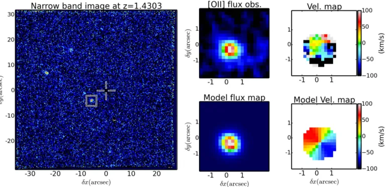
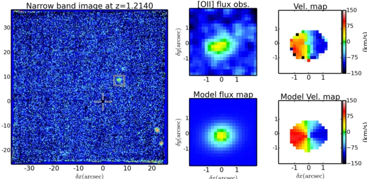
Figures2–7 show GalPaK3Dreconstructed models as well as Camel velocity maps for the six galaxies in the twofields. In Figure 2 (SDSS J213748+0012 field), the other emission sources are the quasar and a star’s residual continuum. In these
figures, the left panel corresponds to a narrow-band image of 30 pixels (37.5Å) around the galaxy’s [OII] emission lines. The background continuum has been subtracted, so that we can only see the galaxy in emission. In each of these Figures, we see the galaxy (inside the white rectangles) within 15″ of the quasar LOS(represented by a white cross). In the two right columns of these Figures,[OII]integratedflux and velocity maps are shown. The top row corresponds to a 2×2(2 pixels FWHM)spatial Gaussian-smoothedflux map(left)and the Camel velocity map (right). The bottom row shows the GalPaK3Dmodel flux(left) and the PSF-deconvolved velocity(right)maps. We can see that in all cases, except in Figure 3 for the dispersion-dominated SDSS J213748+0012G2 galaxy, the model flux maps from GalPaK3Dare in a good agreement with the observedflux, and that GalPaK3Dand Camel velocity maps are consistent. Table6
lists the resulting parameters for each galaxy.
GalPaK3Dresults are reliable if the central galaxy pixel has, at minimum, an S/N pixel−1of 3 (Bouché et al. 2015). For each galaxy, we have S/N pixel−1of 11.0, 11.0, 4.5, 9.3, 4.2, and 10.5 for SDSS J213748+0012G1, G2, G3 and SDSS J215200+0625G1, G2 and G3, respectively. We checked that
Figure 1.Scheme representing the azimuthal angle: the galaxy is represented at the center in black, the red arrows represent the outflowing gas expelled from both side of the galaxy minor axis. The azimuthal angleαis represented by the blue angle between the galaxy major axis and the quasar LOS(in yellow).
15
The PA of a galaxy is the angle between the galaxy major axis and the celestial north.
16
The source code can be found athttps://bitbucket.org/bepinat/camel.git. 17
the parameters have converged for each galaxy as well as cross-checked on raw data.
3.4. Classification and Notes on the Individual Cases
To put constraints on galactic outflows, we first need to select galaxy–quasar pairs suitable for wind studies (
wind-pairs). To do so, we measure the angle between the galaxy major axis and the apparent quasar location, which is referred to as the azimuthal angle α (see Figure 1). Depending on this angle, the quasar LOS is likely to probe different phenomena around the galaxy. If 55°α90°, the quasar’s position on the sky is roughly along the galaxy minor axis and is likely to cross the outflowing material of
Figure 2.GalPaK and Camel results on galaxy J213748+0012G1. Left: narrow-band image(30 pixels corresponding to 37.5Å)for[OII]λ3727, 3729 at redshift
z=0.8069. The quasar LOS is represented by the white cross and the galaxy is inside the white rectangle. The other spot on the right corresponds to continuum residuals from a star. Right: from left to right:[OII]doublet integratedflux and velocity maps. The top row corresponds to a 2×2 Gaussian-smoothedflux map(the left panel)and Camel velocity map(top right). The bottom row represents the GalPaK3Dmodelflux(left)and PSF-deconvolved velocity maps(right). Color bars on the right show the velocities of the corresponding velocity maps, inkm s-1. This galaxy has a maximum signal-to-noise ratio(S/N)pixel−1of≈11.
Figure 3.Same as Figure2, but for J213748+0012G2 at redshiftz=1.1893. This galaxy has a maximum S/N pixel−1of≈11. For this galaxy, we can see that the
velocity maps do not agree with each other. Because one part of the galaxy is not reproduced by our model and clearly has aflux component(top middle panel), this galaxy seems to be a merger and, therefore, the azimuthal angle of this pair is not reliable.
7
the galaxy18 (e.g., Bordoloi et al. 2011, 2014; Kacprzak et al. 2012, 2014). If a pair has such an azimuthal angle, it will be classified as a wind-pair. On the other hand, if the quasar is positioned along the galaxy major axis (0°α30°), the quasar LOS is likely to probe inflowing or circumgalactic gas. With such a configuration, we classify
the pair as suitable for accretion studies (inflow-pair). In between, (35°α55°), we cannot distinguish between these two extreme cases.
In addition to the azimuthal angle, if a galaxy has a low inclination, classification can be ambiguous given that the uncertainty on the PA will be large. Figure 8 shows galaxy inclination as a function of quasar azimuthal angle. From thefive detected galaxies in the two quasar fields that are non-mergers, two are classified as inflow-pairs, one is an ambiguous case as its
Figure 4.Same as Figure2, but for J213748+0012G3 at redshiftz=1.2140. This galaxy has a maximum S/N pixel−1of 4.5. The spots located bottom right in the narrow-band image corresponds to other galaxies. These galaxies have very low probability to be the host of the MgIIabsorption line in the quasar spectrum as they are located further away from the quasar LOS(212 and 246 kpc).
Figure 5.Same as Figure2, but for J215200+0625G1 at redshiftz=1.0534. This galaxy has a maximum S/N pixel−1of 9.3. The spot located top middle-right in the narrow-band image corresponds to another galaxy. Like the one in Figure4, this galaxy is less likely to be the host of the MgIIabsorption line in the quasar spectrum as it is located further away from the quasar LOS(189 kpc).
18
azimuthal angle is 47°, one is a face-on galaxy and only 1 (J215200+0625G2)can be robustly classified as a wind-pair.
3.4.1. SDSS J213748+0012G1 Galaxy
The first detected galaxy(“G1”)in the SDSS J213748+0012 quasar field(Figure2)has an impact parameterb≈88 kpc and corresponds to the zabs≈0.8063 MgII absorption lines with a
REW Wrl2796 of 0.789Å. This J213748+0012G1 galaxy is inclined by i≈49±1.4° and its derived maximum rotation velocity isVmax≈127±5km s-1. With an[OII]integratedflux
of 8.7×10⁻¹⁷erg s−1cm−2, its SFR is≈6.3±0.7Myr-1. In
Figure2, it can be seen that the morphology and the PA are well reproduced by GalPaK3D. The azimuthal angleαwith the quasar LOS isα=25 deg, i.e., the LOS is aligned with the major axis.
3.4.2. SDSS J213748+0012G2 Galaxy
The galaxy J213748+0012G2 (Figure 3) corresponding to thezabs≈1.1890 MgIIabsorption lines with a REWWrl
2796of
0.308Åin the J213748+0012 quasar spectrum, has an impact parameter of b≈64 kpc and a total [OII] doublet flux of 1.47×10⁻¹⁶erg s−1cm−2. From the[OII]integratedflux we derive an SFR of≈41±8.0Myr-1. This galaxy has a large
velocity dispersion σ≈114±2.3km s-1, i.e., it is a disper-sion-dominated system with V/σ∼0.2. Furthermore, the velocity field derived from the line-fitting algorithm Camel does not agree with its morphology, i.e., its morphological and kinematic main axes are strongly misaligned, by ≈80° (Figure 3). This is a strong indication for a merger, and therefore, this galaxy will not be considered as a wind case, since the PA of this galaxy is ambiguous.
3.4.3. SDSS J213748+0012G3 Galaxy
The other galaxy (J213748+0012G3, Figure 4) from the J213748+0012 field corresponding to the MgII absorption lines at redshift zabs≈1.2144 and a REWWrl
2796 of 1.144Å
has an impact parameter b of ≈87kpc. This galaxy has an inclination i≈40±5°, a maximum rotational velocity Vmax≈166±18km s-1, and an [OII] flux of 4.17×
10−17erg s−1cm−2. From this flux, we derive an SFR of
≈8.9±1.1Myr-1. In contrast to J213748+0012G2, the
kinematic and morphological PAs agree well(Figure4), hence the 3D GalPaK3Dmodel accounts for the 3D emission of this galaxy. In this case, the quasar LOS is at≈45°from the major axis of this galaxy, and this pair is thus classified as ambiguous.
3.4.4. SDSS J215200+0625G1 Galaxy
The first detected galaxy from the SDSS J215200+0625 quasarfield corresponds to the MgIIabsorption lines at redshift zabs∼1.0534 with a REW Wrl
2796 of 0.545Å. This galaxy
(J215200+0625G1) has an impact parameter b≈45 kpc, a maximum rotational velocity Vmax≈161±2km s-1, and an
inclination i≈69°±0°. 7. With an [OII] integrated flux of 1.09×10⁻¹⁶we derive an SFR of≈19.0±3.1Myr-1. For
this galaxy, Figure 5 shows a good agreement between the GalPaK3Dand Camelflux and velocity maps. We can clearly see that the quasar LOS is aligned with the major axis of this galaxy withα=4 deg, and is thus classified as an inflow-pair.
3.4.5. SDSS J215200+0625G2 Galaxy
The galaxy(J215200+0625G2)19corresponding to the redshift zabs≈1.3190 MgII absorption lines with a REW Wrl2796 of
1.424Åhas an impact parameterb≈34 kpc. The derived galaxy redshift is 1.31845 with an inclination of i≈59±11° and a maximum rotational velocity Vmax≈130±29km s-1. With an
[OII]flux of≈1.99×10⁻¹⁷erg s−1cm−2, we derive an SFR of
≈4.6±0.4Myr-1. Even if this galaxy is faint, as can be seen
in Figure 6, its GalPaK3D-derived morphology and PA are in
Figure 6.Same as Figure2, but forJ215200+0625G2at redshiftz=1.3184. This galaxy has a maximum S/N pixel−1of 4.2 and is thus difficult to see in the left image, but can be seen in the smoothed[OII]flux image.
19
In the paper(text, tables andfigures), the only wind-pair will appear in bold font to help the reader.
9
good agreement with Camel maps. The quasar LOS is aligned with the minor axis of this galaxy withα=88±5 deg.
3.4.6. SDSS J215200+0625G3 Galaxy
The last galaxy (J215200+0625G3) in the J215200+0625 quasar field has an impact parameter b≈63 kpc and corresponds to the MgII absorption lines at redshift zabs≈1.4309 with Wrl =1.152
2796
Å. The galaxy has an inclination of i≈13±4°, a maximum rotational velocity Vmax≈298±40km s-1, and an [OII] integrated flux of
≈5.05×10⁻¹⁷erg s−1cm−2. With thisflux, we derive an SFR of≈19±3.0Myr-1. Figure7shows that the morphology is
in agreement with Camel, but the PA derived for this galaxy is more uncertain due to the low inclination of this galaxy. With an azimuthal angle ofα=72±20 deg and its low inclination, we cannot determine whether the quasar LOS is aligned with the minor or major axis of the galaxy.
3.5. Radial Dependence of CGM
For each quasar spectrum, we measure the REW for the MgIIabsorption lines(Wrl2796)in the UVES data and compare
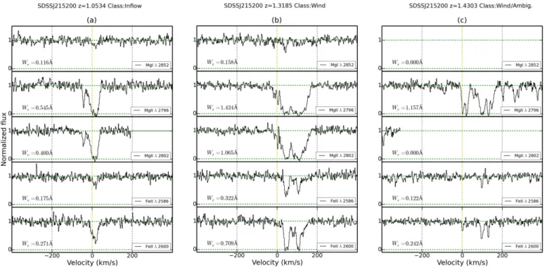
them with the SDSS valuesWrl2796(see Table7). Wefind that the results are consistent with each other. We also calculate REWs of the MgIIλ2803, MgIλ2852, FeIIλ2586, and FeII λ2600 in UVES quasar spectra. Results are shown in Table7. Figures 9 and 10 show the UVES MgIλ2852, MgII λλ2796,2802, and FeII λλ2586,2600 absorption profiles and label the measured REW of each profile for both quasarfields. One of thefirst deductions we can make from Figures9and
10is that there is no clear difference(like different asymmetry behavior for instance) between what seems to be outflowing material and circumgalactic or inflowing gas concerning the different absorption lines.
Figure11 shows the distribution of REWWrl2796 for pairs with an azimuthal angle α>45° as a function of impact parameter b for this work as well as Kacprzak et al.(2011a,
2011b)and Schroetter et al.(2015). This Figure shows that for wind-pairs, as mentioned in Bouché et al.(2012), we clearly see a tight correlation betweenWrl2796 and b. This Wrl2796–b
correlation goes approximatively asb−1. Thisfigure shows that the anticorrelation between impact parameterbandWris again confirmed at b<100 kpc. The scatter around the relation in Figure11is ≈0.3 dex(delineated with the dotted lines). The
Figure 7.Same as Figure2, but for J215200+0625G3 at redshiftz=1.4303. Note that the emissions around the galaxy in the observed[OII]flux panel is noise and not tidal tails. This galaxy has a maximum S/N pixel−1of 10.5. Again, as in Figures4and5, residual spots are galaxies further away from the quasar LOS and are thus less likely to be the host of the absorbing materials(78, 184, and 211 kpc). The 78kpc away galaxy is close enough to be considered as a host galaxy, but we choose to ignore it based on impact parameter argument.
Figure 8.Galaxy inclinations as a function of azimuthal angleαfor thefive nonmerger galaxies detected in the two fields J213748+0012 and J215200
solid line traces the fiducial 1/b relation for mass-conserved biconical outflows(see Bouché et al.2012).
4. WIND MODEL
In this section, we describe the wind modeling. We create a cone with an opening angle corresponding20toθmaxand fill it randomly with particles representing cold gas clouds being pushed away by a hot medium or radiation pressure. These particles are distributed such that their number goes like 1/r2, whereris the distance to the galaxy center. The particle density is normalized arbitrarily to reproduce the optical depth of the absorption profiles.
Such entrained clouds are accelerated to their terminal velocity quickly in a few kpc or<10 kpc, since the pressure from the hot medium or the radiationfield scales as 1/r2. The range of impact parameters for the galaxy−quasar pair in our sample is always
larger than 30kpc. Hence, we assume, for simplicity, that the particles have a constant radial velocity corresponding toVout. In
addition, a single LOS probes a rather small range of distances from the host galaxy such that a gradient in the outflow velocity would have no significant impact on our results. So far, only in one LOS with an impact parameter less than 10 kpc in Schroetter et al.(2015), did we require an accelerated wind profile.
We then orient the cone following the galaxy inclination and simulate the quasar LOS such that the galaxy–quasar pair matches the geometrical configuration of the MUSE data.
The particle velocities are then projected along the simulated quasar LOS and the distribution of the projected velocities gives us a simulated optical depthτv, which we turn into an absorption profileµexp(-tv). In order to facilitate comparison with the data, Poisson noise is added to the simulated absorption profile to simulate the instrumental noise. This noise is chosen to have the same level as the data.
The model has two main free parameters, the wind speed Vout and θmax the wind opening angle. These two parameters
Table 7
UVES Rest Equivalent Widths
Galaxy Wrl2796(SDSS) Wrl2796 Wrl2802 Wl
r2852 Wrl2586 Wrl2600 log(NHi) Class
(1) (2) (3) (4) (5) (6) (7) (8) (9)
J213748+0012G1 0.724±0.09 0.789±0.02 0.572±0.02 0.145±0.02 0.135±0.02 0.309±0.02 19.24 Inflow J213748+0012G2 0.308±0.06 0.294±0.02 0.155±0.02 0.039±0.02 L 0.058±0.02 18.61 Merger J213748+0012G3 1.122±0.06 1.132±0.02 1.040±0.02 0.223±0.02 0.707±0.02 0.947±0.02 19.58 Ambig. J215200+0625G1 0.522±0.14 0.545±0.02 0.460±0.02 0.116±0.02 0.175±0.02 0.271±0.02 19.01 Inflow
J215200+0625G2 1.347±0.12 1.424±0.02 1.065±0.02 0.158±0.02 0.322±0.02 0.709±0.02 19.71 Wind J215200+0625G3 1.152±0.11 1.157±0.02 L L 0.122±0.02 0.242±0.02 19.59 Wind/Ambig.
Note.(1)Quasar name;(2)SDSS MgIIλ2796 REW(Å);(3)UVES MgIIλ2796 REW(Å);(4)UVES MgIIλ2803 REW(Å);(5)UVES MgIλ2852 REW(Å);(6) UVES FeIIλ2586 REW(Å);(7)UVES FeIIλ2600 REW(Å);(8)Gas column density at the impact parameter(cm−2);(9)Class(inflow-pair/wind-pair)based onα selection.
Figure 9.UVES MgIλ2852, MgIIλλ2796, 2802, and FeIIλλ2586, 2600 absorption lines centered at host galaxy systemic velocity for the SDSS J213748+0012 quasar spectrum. The left panel corresponds to absorption lines from the SDSS J213748+0012G1 host galaxy(a). The middle panel to the SDSS J213748+0012G2 host galaxy(b), and right panel to SDSS J213748+0012G3(c). Note that in the right column, the FeIIλ2586 REW is calculated without the≈200km s-1absorption
component.
20
θmaxis defined from the central axis, and the cone subtends an area Ω
ofp q· max2 .
11
are independent for a given galaxy inclination, as one can see from the following arguments(see also Schroetter et al.(2015)
for more details). The outer edges of the absorption profile (reddest for a cone pointing away from the observer, bluest for a cone pointing toward the observer) depend directly on the wind velocity(Figure A-1 in Schroetter et al.2015). The inner edge (toward Vsys)of the absorption profile depends directly on the wind opening angleθmax(Figure A-1 in Schroetter et al.
2015). Note that the galaxy inclination impacts the absorption profiles similarly to the θmax parameter, but since the inclination is determined by our 3D fit with GalPaK3D, there are no degeneracies.
In order to determine which model best reproduces the data, the best-fit model is visually found. However, given that there
are stochastic features in the simulated profiles, we generate dozens of simulated profiles for a given set of parameters. The errors on these parameters are given by the range of values allowed by the data. We proceed as follows: Wefirst generate models, changing only one parameter to fit one part of the absorption profile (outer part for Vout or inner part for θmax).
Then, we change only the other parameter (θmax or Vout)
generating other models tofit the other part of the absorption. We generate models with a range of values of 10–500km s-1 (with steps of 10km s-1)for V
out and 20°–50°(with steps of
5°)for θmax. As mentioned before, with these two parameters being independent, there is no degeneracy between the generated models. We use these parameter ranges to fit the data, since outflows are likely to be collimated in a cone with an opening angle around 30°(e.g., Chen et al.2010; Bordoloi et al.2011, 2014; Bouché et al. 2012; Kacprzak et al. 2012; Martin et al.2012; Rubin et al.2014)
Examples on how the wind model behaves, as we change the different parameters, can be seen in the appendix of Schroetter et al.(2015).
4.1. The Wind-pair Case of J215200+0625G2
Figure10, middle column(b), shows the UVES MgIλ2852, MgIIλλ2796, 2802, and FeII λλ2586, 2600 absorption lines for this galaxy–quasar pair. Fromthis Figure, we can see that the MgIIλλ2796, 2802 absorption lines are saturated and thus the need to simulate the absorption from FeIIλ2586, which are the only nonsaturated absorption lines in the presented transitions.
The bottom right panel of Figure12shows the UVES FeII λ2586 absorption lines corresponding to the J215200+0625G2 galaxy redshift of z=1.3184. This absorption is the one we intend tofit in order to constrain outflow properties, since other absorption lines like MgII are saturated (see panel (b) of Figure 10). In this profile, we can see a suppression of
Figure 10.UVES MgIλ2852, MgIIλλ2796, 2802, and FeIIλλ2586, 2600 absorption lines centered at host galaxy systemic velocity for the SDSS J215200+0625 quasar spectrum. The left panel corresponds to absorption lines from the SDSS J215200+0625G1 host galaxy(a). The middle panel to theSDSS J215200+0625G2 host galaxy(b), and right panel to SDSS J215200+0625G3(c).
Figure 11.Wl
r2796as a function of impact parameterbfor galaxy–quasar pairs
classified as wind-pairs. The dashed blue lines show the 0.3 dex scatter. The horizontal dotted black lines represent theWrl2796=0.8ÅandWrl2796=0.5Å
absorption around 80km s-1. We first tried to fit this absorption with our wind model described in Section 4, but failed to reproduce this gap, even with stochastic effects. This lack of absorbing particles at these velocities shows that the outflowing cone must have a low-density region inside it.
Given that the geometry of this galaxy–quasar system(with a galaxy inclinationiof 59°)and that the quasar line of sight is crossing the outflowing cone near its middle(α=88°), we thus developed a partially empty cone model in order to reproduce the absorption profile.
The principle is the same as in the wind model described in Section4, except that we onlyfill the cone with particles from a certain opening angleθintoθmax. The inner cone is thus empty. This model should only work if the azimuthal angle α of a galaxy−quasar system is above∼80°, and thus the quasar LOS is crossing this empty region and creating a gap of velocities in the simulated profile.
This empty inner cone could be the signature of a hotter gas
filling the inner cone, while the ionized gas traced by our low-ionization lines would correspond to the walls of the outflowing cone in a manner similar to Fox et al.(2015) for the Milky Way and to Veilleux & Rupke(2002)for NGC1482. Figure 12 illustrates the resulting wind modeling for this galaxy. The first left column corresponds to the wind model representation. The top left panel shows a[OII]integratedflux, continuum-subtracted image with the orange cross showing the
quasar LOS position. The inclined circles represent the outflowing cone. The bottom left panel represents a side view of the cone, with the quasar LOS being represented by the dashed red line, and with the observer on the left. This representation allows us to see if the outflowing material is ejected toward or away from us, assuming our cone model is representative. The red part of the cone represents the empty inner part.
In the middle column are represented the simulated profiles (top) and UVES spectrum around the absorption line FeII λ2586 (bottom). The red part of the simulated profile is the profile without instrumental noise and the apparent noise is due to stochastic effects from the Monte Carlo particle distribution. The red simulated absorption profile does not change much for the UVES data compared to the noise-added one. We also present in Figure12, top right panel, a similar simulated profile (with the same parameters), but without the empty inner cone model. It can clearly be seen in this Figure that we cannot reproduce the gap shown in the data without an empty region. The bottom middle panel corresponds to UVES data. It corresponds to the QSO spectrum absorption lines centered at the galaxy systemic velocity. The element FeII λ2586, corresponding to the absorption lines, is shown in the bottom middle column panel.
To reproduce the shape of this absorption profile and generate the simulated profile shown in the top middle panel of
Figure 12.Representation of the cone model and quasar spectrum associated with theJ215200+0625G2galaxy(z=1.31845). Top left: the cone model seen in the sky plane(xy). This is a narrow-band image centered around the galaxy[OII]emission lines with the continuum subtracted. The dashed circle represents the inclined galaxy disk and the black and white inclined circles illustrate the gas outflow cone. The orange cross represents the position of the quasar LOS. Bottom left: a side view of the cone, where thez-axis corresponds to the quasar LOS direction with the observer to the left. The red part of the cone represents the empty inner cone. Middle: Normalizedflux for the FeII(λ2586)absorption line observed with UVES(bottom)and the reconstructed profile(top). Note that this model does not reproduce the depth of the absorption line. In the UVES simulated absorption profile, the red line corresponds to the simulated profile without any instrumental noise. This wind model uses a very low-density inner cone, as described in Section4.1. Right: same as the top middle panel, but with no empty inner cone model. This simulated profile has the same parameters as the empty inner cone one. It can clearly be seen that we cannot reproduce the gap in absorptions seen in the UVES absorption profile without the empty cone model. This outflow has aVoutof 150±10km s-1, a cone opening angleθmaxof 20±5°, and an inner opening angleθin
of 7±2°.
13
Figure 12, we adjust the outflow speed Vout and the cone
opening angleθmax, while keeping the geometrical parameters of the galaxyfixed, as described in Section4.
The best values for reproducing the UVES FeII λ2586 absorption profile are an outflow velocity Vout of
150±10km s-1 and a cone opening angle θmaxof 20°±5°. For this specific case, we derive an inner opening angle of the cone ofθin≈7°.
4.2. Outflow Rates
Having constrained the outflow velocity and cone opening angle for the wind-pair, we can now derive the ejected mass rate M˙out as well as the loading factor.
For our wind-pair, the equivalent width of the absorption lines only depends on θmax and Vout (see Section 4). After
testing several opening angles and outflow velocities, wefitted the width of the absorption profile created by gas outflowing from the galaxy. The asymmetry of the profile depends on the
Table 8
Results for the GalaxyJ215200+0625G2
Galaxy b(kpc) log(NH(b)) Vmax Vout θmax SFR M˙out
V V
out
esc η
(1) (2) (3) (4) (5) (6) (7) (8) (9) (10)
J215200+0625G2 34.0 19.7±0.07 140.8±51 150±10 20±5.0 4.6±0.4 1.7-+0.81.1 0.52 0.75
1.1-+0.60.9 0.49
Note.(1)Galaxy name;(2)Impact parameter(kpc);(3)Gas column density at the impact parameter(cm−2);(4)Maximum rotational velocity of the galaxy(km s-1);
(5)Wind velocity(km s-1);(6)Cone opening angle(degrees) (7)SFR(Myr-1);(8)Ejected mass rate for one cone(Myr-1);(9)Ejection velocity divided by
escape velocity;(10)Mass loading factor: ejected mass rate divided by SFR(for both cones). Values in the second row(M˙out=1.1+-0.60.9Myr-1andη=0.49) correspond to the empty inner cone model.
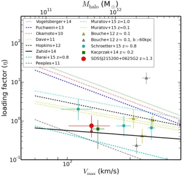
Figure 13. Comparison of mass loading factors assumed by theoretical/ empirical models (curves) with values derived from background quasar observations (dots and triangles)as a function of the maximum rotational velocity. The result from this work is represented by the red circle. The red arrow represents the loading factor of theSDSS J215200+0625G2galaxy with the subtracted mass from the inner cone model. The cyan circles show the results for galaxies atz≈0.8 from Schroetter et al.(2015). The green square shows the mass loading factor for az≈0.2 galaxy(Kacprzak et al.2014). The triangles show the results forz≈0.2 galaxies from Bouché et al.(2012). The gray triangles show the galaxies with quasars located at>60 kpc, where the mass loading factor is less reliable due to the large travel time needed for the outflow to cross the quasar LOS (several 100 Myr) compared to the short timescale of the Hα-derived SFR(∼10Myr). The upper halo mass axis is scaled onVmaxat redshift 0.8 from Mo & White(2002).
Table 9
MUSE Sources in the SDSS J213748+0012 Field with Redshifts
ID R.A. Decl. Redshift Lines
obj001 21:37:48.303 +00:12:21.69 0.132 OIII, Hβ, Hα, NII obj002 21:37:48.757 +00:12:19.29 0.156 OIII, Hβ, Hα, NII obj003 21:37:50.157 +00:12:52.89 0.315 Hβ, OIII obj004 21:37:48.370 +00:12:23.89 0.325 OII, OIII, Hβ,
Hα, NII obj005 21:37:48.370 +00:12:24.09 0.325 OII, OIII, Hβ, Hα obj006 21:37:48.930 +00:12:38.69 0.409 OII, OIII, Hα, NII obj007 21:37:49.223 +00:12:20.09 0.410 OII, OIII, Hβ obj008 21:37:49.810 +00:12:15.69 0.442 OII obj009 21:37:48.477 +00:12:30.09 0.543 OII, OIII, Hβ obj010 21:37:48.450 +00:12:29.49 0.543 OII, OIII, Hβ obj011 21:37:50.450 +00:12:02.89 0.580 OIII, Hβ obj012 21:37:48.983 +00:12:55.09 0.616 OII, OIII, Hβ obj013 21:37:49.343 +00:12:52.09 0.684 OII, OIII, Hβ obj014 21:37:47.743 +00:12:46.69 0.711 OII obj015 21:37:49.530 +00:12:14.69 0.766 OII obj016 21:37:48.317 +00:12:15.69 0.767 OII obj017 21:37:49.463 +00:12:16.49 0.767 OII, OIII obj018 21:37:49.023 +00:12:27.29 0.806 OII, OIII, Hβ obj019 21:37:48.823 +00:12:27.49 0.806 OII, OIII obj020 21:37:50.157 +00:12:30.89 0.806 OII, OIII obj021 21:37:49.490 +00:12:33.69 L 8281.3 obj022 21:37:50.103 +00:12:53.29 L 6823. obj023 21:37:49.117 +00:12:11.89 L 6897. obj024 21:37:47.663 +00:12:12.69 0.900 OII obj025 21:37:48.930 +00:12:09.49 0.902 OII? obj026 21:37:48.517 +00:12:05.69 L 7079.69 obj027 21:37:48.063 +00:12:33.69 L 7376.81 obj028 21:37:48.437 +00:12:46.29 1.010 OII obj029 21:37:48.837 +00:12:42.69 1.010 OII obj030 21:37:48.970 +00:12:09.49 1.045 OII obj031 21:37:49.970 +00:12:09.09 1.044 OII obj032 21:37:49.970 +00:12:15.29 1.122 OII obj033 21:37:48.903 +00:12:17.69 1.188 OII obj034 21:37:46.837 +00:12:02.89 1.212 OII obj035 21:37:47.970 +00:12:29.09 1.213 OII obj036 21:37:46.943 +00:12:08.89 1.214 OII obj037 21:37:47.850 +00:12:33.49 1.214 OII obj038 21:37:50.410 +00:12:20.09 1.257 OII obj039 21:37:48.370 +00:12:04.69 1.300 OII obj040 21:37:47.717 +00:12:46.89 L 8569.12 obj041 21:37:48.730 +00:12:15.29 5.941 8434.53 Lyα? obj042 21:37:48.823 +00:12:27.49 6.442 9043.03 Lyα?
system geometry. To constrain the ejected mass rate probed by the quasar LOS, we use Equation(5)from Bouché et al.(2012)
and Schroetter et al.(2015):
m p q
m
q
»
»
-
-
M N b b V
M M
N b
b V
2
0.5 yr 1.5 10 cm
25 kpc 200 km s 30 5
out H out max
out 1
H
19 2
out 1
max
˙ · ( ) · · · ·
˙
· ( )
· · · ( )
μbeing the mean atomic weight,bthe impact parameter,θmax the cone opening angle,21Voutthe outflow velocity andNH(b)
is the gas column density at the bdistance.
The only parameter, which is yet to be constrained, is the gas column densityNH(b). To do that, we use the empirical relation
between the neutral gas column density and the MgII λ2796 REWWrl2796(Equation6 of Ménard & Chelouche2009):
=
´ ´ l
-
N
W log cm log 3.06 0.55
10 r . 6
H 2
19 2796 1.7 0.26
I
( )( ) [( )
( ) ] ( )
To compute the errors, we assume a Gaussian error distribution. As described in Schroetter et al. (2015), for regions with HI column density above log(NHI)=19.5, the
ionized gas contribution is negligible. Also argued by Jenkins
Table 10
MUSE Sources in the SDSS J215200+0625 Field with Redshifts
ID R.A. Decl. Redshift Lines
obj001 21:52:02.018 +06:25:47.66 0.433 OII, OIII, Hβ obj002 21:52:02.246 +06:25:25.06 0.439 OII obj003 21:51:58.905 +06:25:20.26 0.452 OII, OIII, Hβ obj004 21:52:02.085 +06:25:13.26 0.489 OII, OIII, Hβ obj005 21:51:58.409 +06:24:54.86 0.517 OII obj006 21:51:59.429 +06:25:43.06 0.554 OII, OIII obj007 21:52:02.273 +06:24:56.06 0.597 OII, OIII, Hβ obj008 21:52:00.770 +06:25:17.26 3.931? 5992.37 Lyα? obj009 21:51:59.200 +06:24:54.86 4.196? 6314.05 Lyα? obj010 21:51:58.878 +06:25:01.46 0.742 OII, OIII, Hβ obj011 21:51:59.912 +06:25:15.66 0.748 OII, Hβ obj012 21:52:02.139 +06:25:31.26 0.770 OII, OIII, Hβ obj013 21:51:59.375 +06:25:40.26 0.786 OII
obj014 21:52:00.341 +06:25:22.46 0.332 OII, OIII, Hα obj015 21:52:01.092 +06:25:16.26 0.824 OII, OIII obj016 21:52:00.636 +06:25:37.66 0.289 Hα, NII obj017 21:51:58.597 +06:25:11.86 0.847 OII? obj018 21:51:59.818 +06:25:29.66 0.873 OII obj019 21:52:00.126 +06:25:13.06 0.879 OII, OIII obj020 21:52:00.234 +06:24:50.86 0.438 OII, OIII, Hβ obj021 21:51:59.630 +06:25:40.46 0.943 OII obj022 21:52:00.287 +06:25:06.46 0.989 OII obj023 21:52:02.058 +06:25:40.46 1.013 OII obj024 21:51:58.436 +06:25:04.46 1.013 OII obj025 21:52:00.381 +06:25:20.46 1.052 OII obj026 21:51:59.549 +06:25:39.06 1.053 OII
obj027 21:52:02.380 +06:24:58.06 0.185 OIII, Hβ, Hα, NII obj028 21:51:58.583 +06:25:34.26 L 8413.87 obj029 21:52:00.904 +06:24:50.26 1.302 OII obj030 21:52:00.019 +06:25:13.26 1.318 OII obj031 21:51:59.952 +06:25:15.46 1.318 OII obj032 21:51:58.355 +06:25:03.06 1.349 OII obj033 21:51:58.489 +06:24:59.06 L 8757.32 obj034 21:52:02.354 +06:25:15.46 1.362 OII obj035 21:51:58.355 +06:25:23.66 1.403 OII obj036 21:52:00.435 +06:25:13.46 1.430 OII obj037 21:52:00.623 +06:25:15.86 1.430 OII obj038 21:52:01.629 +06:25:24.06 1.431 OII obj039 21:52:00.972 +06:25:33.06 1.433 OII obj040 21:52:00.703 +06:25:43.06 1.435 OII obj041 21:52:00.180 +06:25:41.26 1.432 OII
Note.Within these 41 galaxies, 40 have identified emission lines.
Figure 14. Red giant branch image of the J213748+0012 field with identifications of emission-detected galaxies. The white cross points out the quasar location. Circles represent emission-detected galaxies corresponding to Table9. Not all the galaxy-like spots are circled on the image. These spots are either stars or galaxies with a continuum, but without obvious emission line.
Figure 15.Same as Figure14, but for the J215200+0625 quasarfield. Again, the white cross shows the quasar location, and galaxies with emission lines are circled and listed in Table10.
21
We remind the reader thatθmaxis defined in Section4.
15
(2009), if this column density is above this limit, one can use the correlation between the MgIIequivalent width andNHIas a
proxy for the NH gas column density. For the wind-pair
J215200+0625G2, we have a gas column density oflog(NHI)»19.70.07.
Another aspect of outflow properties is whether the outflowing gas is able to escape from the galaxy gravitational well. To determine this, we derive the escape velocityVescfor
the J215200+0625G2 galaxy. The escape velocity for an isothermal sphere is defined by Equation (7) (Veilleux et al.2005).
⎜ ⎟ ⎡ ⎣⎢ ⎛ ⎝ ⎞⎠ ⎤ ⎦⎥ = +
V V R
r
2 1 ln 7
esc max
vir
· ( )
Vmaxbeing the maximum rotation velocity of the galaxy andRvir
its virial radius. The virial radius of the galaxies can be defined as Rvir≈Vmax/10H(z), where H(z) is the Hubble parameter at
redshiftz. In Table8, we compare the outflow velocity with the escape velocity for the wind-pair. This ratio Vout/Vesc of 0.52
shows that the outflowing material is not able to reach the escape velocity and thus will be likely to fall back onto the galaxy, assuming we are tracing the gas going out of the galaxy. One can ask whether we are already tracing the gas falling back onto the galaxy. If this is the case, we should see another opposite component (with respect to the systemic velocity) in the absorption profile corresponding to the outflowing gas.
Table8 also lists the estimated outflow rate. The errors on the ejected mass rateM˙outare dominated by the ones on the gas column density NHIand the SFR.
From the outflow rate, we compute the mass loading factorη by comparing it to the SFR (h =M˙out SFR). For our SDSS
J215200+0625G2 pair, we used the empty cone model to reproduce the absorption profile with an inner cone opening angleθinof 7°. To be consistent with the other cases, we give two solutions for this galaxy−quasar pair: one with the filled cone and one with the inner cone subtracted.
Figure13 shows the loading factorη as a function of halo mass and maximum rotational velocityVmaxfor this work and
previous similar studies (Bouché et al. 2012; Kacprzak et al.2014; Schroetter et al.2015). The derived loading factor for galaxySDSS J215200+0625G2follows the same trend as the others. The red arrow shows the loading factor for the subtracted mass from the low-density inner cone.
MUSE allows us to probe galaxies with an impact parameter larger than before with an IFU. But, in Figure13, we caution the reader that the loading factor for galaxies with impact parameters larger than 60 kpc are less reliable, because of the time needed for the gas to travel from the galaxy to the quasar LOS (∼400 Myr at Vout≈150km s-1 with b=60 kpc). A
major limitation for the comparison between data and models in Figure13, is thatηin simulations are usually measured on a scale of a few kpc away from the galaxy, which is one order of magnitude lower than most of the observations(tens of kpc).
5. SUMMARY
We present results on two GTO VLT/MUSEfields in which we searched for galaxy–quasar pairs. Thesefields were selected from the SDSS database, where we searched for multiple MgII
absorbers, withz≈0.8–1.4 andWrl2796>0.5Å, in the quasar
spectra. Out of eight MgIIabsorptions in the quasar spectra of
these two fields, we detect six redshift-corresponding SFGs. For these twofields(J213748+1112 and J215200+0625), we also have high-resolution spectra of the quasars from the VLT/ UVES instrument. In each of these two fields, we detected more than 40 emitters in the 1′×1′MUSEfield of view(see the Appendix). We focused on galaxies at MgII absorption redshifts in the quasar spectra and for which the associated quasar LOS is aligned with their minor axis (α>55°) and is thus likely to probe outflowing materials(wind-pairs). Among the six detected SFGs, one is likely to be a wind-pair due to its orientation with respect to its relative quasar.
In summary, thanks to our new GTO VLT/MUSE and VLT/UVES data, MUSE allows us to detect galaxies far away from their associated quasar(∼100 kpc)compared to previous similar works (i.e., Bouché et al. 2012; Kacprzak et al.2014; Schroetter et al. 2015). For the wind-pair SDSS J215200
+0625G2, we found that the outflow velocity Vout is ≈150km s-1. The outflowing gas is likely to stay inside the gravitational well of the galaxy and the loading factor is
η≈0.7. We showed a gap in velocities in the absorption profile, which led to a low-density inner cone modeling. At this point, we have outflowing constraints for one galaxy, but we showed that MUSE is able to provide very good data and will play a fundamental role in thisfield.
MUSE allowed us to probe multiple galactic wind cases at the same time and enhance the number of cases with only two quasarfields. We also have a case of low-density inner cone, which opens discussions on geometrical properties of
out-flowing materials. The MEGAFLOW sample is currently growing and is successful in detecting galaxies in each quasar
field (≈84% detection). Future work will be done with a lot more observation with MUSE+UVES, and in a short time, the MEGAFLOW sample should be large enough to produce statistical results on outflow properties.
N.B. acknowledges support from a Career Integration Grant (CIG) (PCIG11-GA-2012-321702) within the 7th European Community Framework Program. This work has been carried out thanks to the support of the ANR FOGHAR ( ANR-13-BS05-0010-02), the OCEVU Labex (ANR-11-LABX-0060) and the A*MIDEX project (ANR-11-IDEX-0001-02) funded by the“Investissements d’Avenir”French government program managed by the ANR. This work received financial support from the European Research Council under the European Unions Seventh Framework Programme (FP7/2007-2013)/ ERC Grant agreement 278594-GasAroundGalaxies.
APPENDIX
MUSE FIELDS’EMITTERS DETECTION
For completeness, we looked for these emitters by visual inspection and found 42 galaxies with emission lines in each of these two fields (see Table 9 for SDSS J213748+0012 and Table10for SDSS J215200+0625).
REFERENCES
Aguirre, A., Hernquist, L., Schaye, J., et al. 2001,ApJ,561, 521
Alam, S., Albareti, F. D., Allende Prieto, C., et al. 2015,ApJS,219, 12
Bacon, R., Bauer, S., Boehm, P., et al. 2006,Proc. SPIE,6269, 62690J
Bacon, R., Bauer, S., Brau-Nogué, S., et al. 2009,ASSP,9, 331
Barai, P., Monaco, P., Murante, G., Ragagnin, A., & Viel, M. 2015,MNRAS,
447, 266

![Figure 2. GalPaK and Camel results on galaxy J213748+0012G1. Left: narrow-band image (30 pixels corresponding to 37.5 Å) for [O II ] λ3727, 3729 at redshift z =0.8069](https://thumb-us.123doks.com/thumbv2/123dok_us/8271881.2190886/7.918.74.853.77.444/figure-galpak-camel-results-galaxy-pixels-corresponding-redshift.webp)
![Figure 6. Same as Figure 2, but for J215200 +0625G2 at redshift z=1.3184. This galaxy has a maximum S/N pixel −1 of 4.2 and is thus dif ficult to see in the left image, but can be seen in the smoothed [O II ] flux image.](https://thumb-us.123doks.com/thumbv2/123dok_us/8271881.2190886/9.918.82.849.80.450/figure-figure-redshift-galaxy-maximum-ficult-image-smoothed.webp)