Hardware design optimization for human motion tracking systems

(1)

Hardware Design Optimization

for

Human Motion Tracking Systems

by

Bonnie Danette Allen

A dissertation submitted to the faculty of the University of North Carolina at Chapel Hill in partial fulfillment of the requirements for the degree of Doctor of Philosophy in the

Department of Computer Science.

Chapel Hill 2007

Approved by

Advisor: Gregory F. Welch

Reader: Gary Bishop

Reader: Henry Fuchs

Reader: Russell M. Taylor II

Reader: Leandra Vicci

(2)

ABSTRACT

BONNIE DANETTE ALLEN: Hardware Design Optimization for

Human Motion Tracking Systems

(Under the direction of Gregory F. Welch)

A key component of any interactive computer graphics application is the system for tracking user or input device motion. An accurate estimate of the position and/or orientation of the virtual world tracking targets is critical to effectively creating a convincing virtual experience. Tracking is one of the pillars upon which a virtual reality environment is built and it imposes a fundamental limit on how real the “reality” of Virtual Reality can be.

(3)

designers to predict or develop intuition about the expected performance impact of adding, removing, or moving source/sensor devices, changing the device parameters, etc.

This research introduces a stochastic framework for evaluating and comparing the ex-pected performance of sensing systems for interactive computer graphics. Incorporating models of the sensor devices and expected user motion dynamics, this framework enables complimentary system- and measurement-level hardware information optimization, inde-pendent of algorithm and motion paths. The approach for system-level optimization is to estimate the asymptotic position and/or orientation uncertainty at many points throughout a desired working volume or surface, and to visualize the results graphically. This global performance estimation can provide both a quantitative assessment of the expected per-formance and intuition about how to improve the type and arrangement of sources and sensors, in the context of the desired working volume and expected scene dynamics. Us-ing the same model components required for these system-level optimization, the optimal sensor sampling time can be determined with respect to the expected scene dynamics for measurement-level optimization.

Also presented is an experimental evaluation to support the verification of asymptotic analysis of tracking system hardware design along with theoretical analysis aimed at sup-porting the validity of both the system- and measurement-level optimization methods. In addition, a case study in which both the system- and measurement-level optimization meth-ods to a working tracking system is presented.

Finally, Artemis, a software tool for amplifying human intuition and experience in tracking hardware design is introduced. Artemis implements the system-level optimiza-tion framework with a visualizaoptimiza-tion component for insight into hardware design choices. Like fluid flow dynamics, Artemis examines and visualizes the “information flow” of the source and sensor devices in a tracking system, affording interaction with the modeled devices and the resulting performance uncertainty estimate.

(4)

ACKNOWLEDGEMENTS

As a civil servant at the National Aeronautics and Space Administration (NASA) Lan-gley Research Center (LaRC), I had the opportunity to pursue a Ph.D. as part of LaRC’s Graduate School Program. In the Fall of 1999, I handed off my project design work and began the first of four semesters on campus at UNC Chapel Hill. During that time, I joined the tracker research group, found a mentor and advisor, formed a committee and proposed. This tremendous progress was made possible through the efforts of many people, some of whom I thank specifically below but there are many more who contributed in more ways than I can enumerate. In 2001, I moved back to NASA LaRC where I went back to project work fulltime and focused on my research between projects and as my personal schedule permitted. This meant that spans of time would pass when I was unable to make research progress and I am grateful to everyone at UNC who helped me to stay focused and advanced the research in my absence.

(5)

and is the product of all contributors. When I refer to “we” or “our” and am not refer-ring to the reader, I am referrefer-ring to all of the contributors to this research but especially to collaboration with Dr. Greg Welch.

There are so many people who helped me along the way that I know I run the risk of forgetting someone in any attempt to acknowledge specific individuals. With apologies in advance to anyone I have overlooked, I want to express my gratitude to the following people:

• my advisor, Greg Welch, for his unwavering enthusiasm and many ideas,

espe-cially the idea of steady-state covariance as a performance metric.

• my Committee as a whole for their continued support of my stop-and-go research

while working full time.

• Gary Bishop for sharing his uncanny ability for making the most complicated

concepts seem intuitive.

• Henry Fuchs for always taking the time to stop by when he saw me in Sitterson to

offer his support and encouragement.

• Russell Taylor for his feedback on my defense practice talk and his “expert”

dis-cussion.

• Leandra Vicci for her insights into the murky world of analog noise and her always

interesting and educational “tangents”.

• Mary Whitton for her heroic efforts leading up to my defense and invaluable

ap-plication focus.

• Marcel Prastawa and Erica Stanley for advancing the research with their work on

the Artemis prototypes.

• Adrian Ilie for his assistance with the 3DMC setup and DragonFly camera data

acquisition.

• John Thomas and David Harrison for their advice and assistance in setting up

experiments.

(6)

• Tim Quigg, Janet Jones and Karen Thigpin for always finding a desk for me,

helping with registration and making sure I had the forms I needed while studying remotely.

• Nick Englund and Ben Elgin of 3rdTech, Inc. for access to the inner workings of

the HiBall tracking system and unending patience for my barrage of questions.

• Duane Armstrong, NASA LaRC’s analog guru, for continuing to take my calls to

answer my many questions about noise.

• George Allison, the head of LaRC’s Graduate School Program, for seeing me (and

others) through the program in the face of funding cuts.

And on a more personal note:

• Michael Nelson for his love and support. It’s been a long road and you can finally

rest easy. I’m finished.

• My parents, Tom and Bonnie Allen, for allowing their grown daughter (and her

dogs!) to intermittently move back in with them from 1999 to 2007.

• My sister and best friend, Julianne Allen, for always being there.

Financial support for this work came from:

• NASA Langley Research Center (LaRC) Graduate School program

• National Science Foundation Information Technology Research grant IIS0121657,

“Electronic Books for the Tele-Immersion Age: A Paradigm for Teaching Surgical Procedures”

• National Library of Medicine (NIH) contract N01LM33514, “Telepresence for

Medical Consultation: Extending Medical Expertise Throughout, Between and Beyond Hospitals”

• DARPA DSO contract for “Wide Area Visuals for a Simulator in a Box”, Award

(7)

• National Science Foundation grant “High-Fidelity Tele-Immersion for Advanced

Surgical Training”, UNC/UPenn/Brown, with Henry Fuchs, Kostas Danillidis, and Andy van Dam.

• Naval Research Lab contract “Technology for Full-Body Tracking”, with Gary

Bishop. Larry Rosenblum, NRL program manager.

The motion capture data used in this thesis was obtained from mocap.cs.cmu.edu [22]. The CMU database was created with funding from NSF EIA-0196217.

The charm and challenge of life and human tracking.

(8)

LIST OF FIGURES

Figure 1.1. The traditional tracking system design process . . . 3

Figure 1.2. An Example Art Gallery . . . 5

Figure 1.3. Computed pressure contours on the body surface, a wing cross-sectional plane and surface oil-flow patterns for a generic business jet configuration (left) and an Blade Acoustic Pressures (right). Both visualizations courtesy of NASA LaRC. . . 6

Figure 1.4. Two volume visualizations of the “flow” of acoustic sensor information in the tracking domain . . . 7

Figure 1.5. Hardware Optimization (in red) integrated into the traditional tracking system design process . . . 10

Figure 1.6. A simple acoustic 3D position tracker example. . . 14

Figure 1.7. Phases of Modeling and Simulation: Qualification, Verification and Validation (QV&V) [2] . . . 14

Figure 2.1. Example of visualized error in the Constellation tracker [38] . . . 18

Figure 2.2. Accelerometer output while walking (top) and context detection performance (bottom) [57]. The vertical axis label on the bottom plot was added for clarification. . . 20

Figure 2.3. Tracking performance of magnetic (left) and inertial (right) systems [43] . . . 21

Figure 2.4. ThePandoraInteractive Camera Placement and Visibility Simulator [89] . . . 21

Figure 2.5. Example of visualized mean radial spherical errors [73] . . . 23

Figure 2.6. Visualizations of position [62] and rotation [61] error from calibration of Ascension’s Flock of Birds for use in Augmented Reality environments . . . 24

Figure 2.7. Organ pipe sources with performer and audience cut planes (left) and time delay isosurface (right) [55] . . . 25

Figure 2.8. Sound Clarity in (from left to right) fan-shaped, box-shaped and reverse-fan-shaped concert halls [91] . . . 26

(14)

Figure 2.9. Example of error (3D uncertainty) vs. number of cameras surrounding

a sphere with and without occlusion [24] . . . 27

Figure 3.1. The Qualification Process . . . 29

Figure 3.2. Traditional Motion Models . . . 32

Figure 3.3. Boxing Motion Capture right hand y-axis data (from top to bottom) position, velocity, acceleration and jerk . . . 35

Figure 3.4. Block diagram of a linear stochastic dynamic system in discrete time (based on a Figure in [42]). Both ¯u_kvectors are zeroed because there is no controllable input. . . 37

Figure 3.5. DARE Existence Test Flow . . . 53

Figure 4.1. Artemis: The Computational Model . . . 58

Figure 4.2. Artemis Functional Architecture . . . 59

Figure 4.3. Artemis Parameter Interaction GUI with sliders and text boxes . . . 61

Figure 4.4. Artemis GUI . . . 63

Figure 4.5. Artemis input file for volume (left) and surface (right) system analysis 65 Figure 4.6. Artemis input file (.INT) for intrinsic parameters . . . 67

Figure 4.7. Artemis grouping specification in EXT input file . . . 69

Figure 4.8. Acoustic Isosurface for -1.76 log meters (left) and -1.6 log meters (right) . . . 72

Figure 4.9. Acoustic Interval Volume for -1.77 to -1.4 log meters (left) and -1.4 to -1.08 log meters (right) . . . 73

Figure 4.10. Acoustic Image Plane at z=0.6 and 0.4 and x = 0.35 meters . . . 73

Figure 4.11. Patient Biopsy in Pandora. . . 74

Figure 4.12. Patient Biopsy in Artemis withP∞_{performance on the left and camera} coverage shown on the right. . . 74

(15)

Figure 5.2. Experimental setup. Left: shows the LED strips on ceiling, the precision 80/20TM rail, the mobile rail supports, and the sliding HiBall sensor fixture (see also the inset). Right: the tape on the floor marks the 28 different linear rail paths that collectively form a grid intended to span the edge of the ceiling (dashed red line) and some portion of the interior. . . 77

Figure 5.3. P∞_{estimates at Left: 1.9 meter “head” height, and Right: 1.0 meter}

“waist” height . . . 79

Figure 5.4. P∞_{volume analysis with image planes for full (left) and sparse (right)}

ceilings . . . 79

Figure 5.5. Rail Deflection Formulas for (right) distributed load and (left) a point load . . . 80

Figure 5.6. Rail Deflection Behavior [1] . . . 81

Figure 5.7. Comparison of measured HiBall position stddev withP∞ _estimates.

Top: position stddev (from curve fit) of the real system. Bottom: P_∞estimates over a plane fit to the rail data. . . 82

Figure 5.8. Comparison of measured HiBall position stddev (top) withP∞_estimates

(bottom) when alternating rows of LEDs are disabled. See also caption for Figure 5.7. 84

Figure 5.9. The 3DMC equipment setup. . . 85

Figure 5.10. 3DMC test setup and Camera Views. . . 85

Figure 5.11. Standard Deviation of 1D Gaussian Blobs. . . 86

Figure 5.12. Standard Deviation of 1D Gaussian Blobs as measured (top) and as estimated (bottom). . . 88

Figure 5.13. Absolute difference in measured and estimated performance. . . 89

Figure 5.14. TheP∞_{analysis of an 8-camera vision-based acquisition rig. The grey}

camera icons indicate accurate positions and rotations of the cameras. . . 90

Figure 5.15. A P∞ _{visualization for a hypothetical hybrid system with acoustic}

devices and cameras. Acoustic transmitters and cameras are depicted with small red and gray icons. . . 92

Figure 5.16. A hypothetical eight-camera motion capture system. Left: picture depicting the arrangement of the eight cameras in the room. Center: volume

(16)

visualization of P∞ _{throughout the space. Right: Surface plot at plane of peak}

performance (z=5.6 ft). . . 93

Figure 6.1. The Verification Process . . . 94

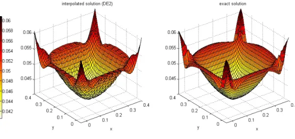
Figure 6.2. Coarse grid solution vs. the exact solution . . . 99

Figure 6.3. Fine grid solution vs. the exact solution . . . 99

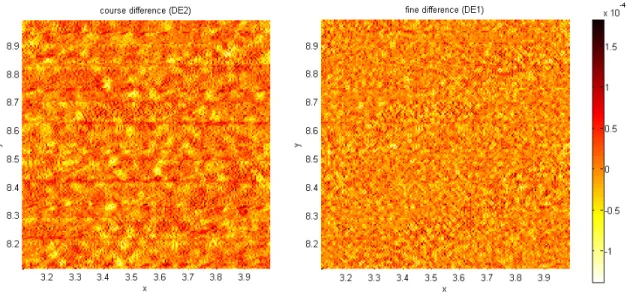
Figure 6.4. Difference between two mesh level and the “exact” solution . . . 100

Figure 6.5. Coarse grid solution vs. the exact solution . . . 100

Figure 6.6. Fine grid solution vs. the exact solution . . . 101

Figure 6.7. Difference between both mesh levels and the “exact” solution . . . 101

Figure 6.8. Coarse grid solution vs. the exact solution with denser sampling . . . . 102

Figure 6.9. Fine grid solution vs. the exact solution with denser sampling . . . 102

Figure 6.10. Difference between both denser mesh levels and the “exact” solution 103 Figure 6.11. The (false) impact of changing dt on the Acoustic System performance 106 Figure 6.12. Noise Density of the LT1124CSB op amp . . . 108

Figure 7.1. The HiBall-3000 . . . 110

Figure 7.2. HiBall P∞ _{estimates rotated 10, 20 and 30 degrees (top to bottom)} around x-axis. . . 112

Figure 7.3. HiBall P∞ _{estimates rotated 10, 20 and 30 degrees (top to bottom)} around y-axis. . . 114

Figure 7.4. HiBall P∞ _{estimates rotated 10, 20 and 30 degrees (top to bottom)} around z-axis. . . 115

Figure 7.5. Full (upper) and Half (lower) Performance with Current (6 LEPD) HiBall Configuration . . . 117

Figure 7.6. P∞_{results for the “checkerboard” ceiling strip pattern . . . 118}

Figure 7.7. Analysis of HiBall measurement noise vs. potential process noise . . . 122

(17)

Figure 7.9. The HiBall Sensor LEPD Configuration [106] . . . 124

Figure 7.10. Current (6 LEPD on top) and Proposed (4 LEPD on bottom) HiBall LEPD configurations with sensor top view on the left and sensor side view on the right . . . 125

Figure 7.11. Full (top) and Half (bottom) Performance with current (6 LEPD) WFOV HiBall configuration at 1.9 meters . . . 127

Figure 7.12. Full (top) and Half (bottom) Performance with proposed (4 LEPD) WFOV HiBall configuration using primary and secondary views at 1.9 meters . . . 128

Figure 7.13. Full (left) and Half (right) Performance with proposed (4 LEPD) WFOV HiBall configuration using primary views only at 1.9 meters . . . 129

Figure 8.1. Effect Size per HiBall Dark-Light-Dark Sample Period from two-sided statistical power analysis . . . 135

Figure 8.2. Number Samples required per HiBall Dark-Light-Dark Sample Period for various net effects . . . 137

Figure A.1. Boxing motion capture right hand y-axis position (top) and velocity (bottom). Note different vertical scale and units. . . 139

Figure A.2. Boxing motion capture right hand y-axis acceleration (top) and jerk (bottom). Note different vertical units. . . 140

Figure D.1. Area in One Tail of the Standard Normal Distribution . . . 163

(18)

LIST OF TABLES

Table 3.1. Stochastic Motion Models . . . 32

Table 3.2. Parameters for P, PV, and PVA Motion Models . . . 41

Table 3.3. Pseudo-code for steady-state evaluation . . . 47

Table 3.4. Existence of the DARE solution [52] . . . 51

Table 6.1. Sensitivity of the Hamiltonian . . . 104

Table 6.2. Values for the (false) impact of changing dt on the Acoustic System performance . . . 105

Table 6.3. Electronic Noise Sources . . . 107

(19)

CHAPTER 1

Introduction

Virtual Reality (VR) is a human-computer interface (HCI) modality that involves real-time simulation and interactions through multiple sensory channels [19], most commonly visual. VR applications immerse the user in a computer-generated virtual environment (VE) that simulates reality through the use of interactive devices, which send and receive information to detect a user’s input and modify the rendered virtual world accordingly. Thus, a VR system or environment can be separated into four components [45]:

• Input

• Simulation

• Rendering

• World Database

If any one of the components does not perform as required, the result is a less than satis-factory virtual experience that can cause a wide variety of negative effects ranging from misinformation (object location for example) to simulation sickness [53].

A key input process into any interactive virtual reality application is the system for tracking user or input device motion. An accurate estimate of the position and/or orien-tation of both people and objects of the virtual world is critical to effectively creating a convincing virtual experience.

(20)

tracking system, the fundamental source of information is the same: pose estimates are de-rived from electrical measurements of mechanical, inertial, optical, acoustic, and magnetic source/sensors [104]. Each type of hardware device has inherent limitations related to the physical medium and practical limitations imposed by the measurement systems. The lim-itations imposed by hardware design affect the rate and quality of the information through-out the working volume for a given system configuration in complex and often unintuitive ways. This complexity often makes it difficult for designers to predict or develop intuition about the expected performance impact of adding, removing, or moving source/sensor de-vices, changing device parameters, etc. For example, what would be the likely effect of removing or re-arranging a tracking system’s optical or acoustic beacons? How and where will the addition of nearby light or sound-occluding objects affect performance? How will moving or redirecting one motion capture camera affect the precision? Will it help to add another camera? How many do you need? What happens if you change the camera lenses or field-of-view (FOV)?

1.1. System Design

Whether working on a new or modified tracking system, designers typically begin the design process with requirements for the size and shape of the working volume, the ex-pected user motion, and the allowable infrastructure. Considering these requirements, they develop a candidate design that includes one or more tracking mediums (optical, acoustic, etc.), medium appropriate source/sensor devices (hardware), and some algorithm (soft-ware) for combining the information from the devices. They then simulate the candidate system in order to estimate the performance for some specific motion paths. This traditional design process is illustrated in Figure 1.1.

(21)

FIGURE1.1. The traditional tracking system design process

design process, it is the choice and configuration of the source/sensor devices (i.e. the hardware) before tracker algorithm selection, and irrespective of the motion paths, that imposes an upper bound on performance. If the necessary information is not available at a sufficient rate and quality throughout the desired working volume, the performance is inherently limited in those areas. In effect the hardware device choices set an upper bound on how well the system as a whole will perform and no estimation algorithm can or should be expected to overcome suboptimal choices of devices, parameters, or geometric arrangement.

(22)

A major aspect of the work in this dissertation is a new hardware design optimization approach to be used prior to the traditional techniques of simulation and prototyping. This hardware design optimization serves to gain insight into the expected overall system per-formance as a function of the hardware choices alone. Ideally, one would specify desired performance goals throughout the working volume, and have a computer search the entire solution space and present the optimal (i.e. minimal) design – a tracking “oracle”. However for all but the most trivial systems the design space is so large as to render such a search intractable, thus making automatic optimization impractical, if not impossible, except in relatively restricted circumstances [74]. This oracle-like approach can be compared to a class of problems known as the Art Gallery problems.

1.2. Problem Complexity

Victor Klee originally posed the problem of determining the minimum number of secu-rity guards sufficient to cover the interior of an n-wall art gallery room [75]. Vasek Chvatal used triangulation to prove thatbn/3cguards are sometimes necessary and always sufficient to cover a two dimensional polygon of n-vertices [26]. Ntafos extended the original Art Gallery problem when he considered the problem of finding the minimal cover for guards in a 2D grid [71]. He found this problem to be solvable in polynomial time. However, he also found that the minimal guard coverage of a three-dimensional grid is NP-complete. A solution for an NP-complete problem can be verified for correctness in polynomial time but cannot be solved in polynomial-time so that every possible solution in a solution set must be tested [28]. As posed by Ntafos, in both the 2D and 3D problems, each point in the plane or volume must be visible by at least one guard without the occlusion by walls as with the original art gallery problem.

(23)

FIGURE 1.2. An Example Art Gallery

measurements. More generally, we need to “see” every point in a tracking volume without interference and we need to see each point more than once because it takes multiple mea-surements to solve for pose. This interference includes the aforementioned occlusion but also includes parameters such as drift in inertial sensors and the effect of ferrous materials on magnetic sensors. Interference can prevent signal reception between sources and sen-sors or degrade it so that the signal is unusable, blinding the system (at least partially) to the occluded points in the tracking volume.

1.3. Intelligence Amplification

Given the intractability of the “oracle” solution, we focus on amplifying human intu-ition and experience in tracking design with a method and tool to be used in conjunction with traditional design techniques and employing a human-in-the-loop approach to “aug-ment the human intellect [beyond that of an] unaided human” [33]. This “intelligence amplification” [6] should help tracking system designers understand the consequences of

(24)

every hardware design specification and decision, their interdependencies and how one may be balanced with another in order to achieve optimum performance [53].

An area where a similar type of intelligence amplification is already in use is com-putational simulation, specifically comcom-putational fluid dynamics (CFD) and finite element modeling (FEM). In CFD, fluid or air-flow visualizations make “invisible” information “visible” as shown in Figure 1.3. Example FEM applications include simulation of elec-tromagnetism, heat transfer, climate, atoms, traffic, and network systems [7]. While the tracking domain discussed here is not CFD or FEM, it does fall into the broader category ofComputational Simulation(see Section 1.6.3). Computational simulation provides qual-itative and quantqual-itative insights into natural phenomena (typically from an area of science or engineering) via mathematics and computer science to gain an improved understanding of a problem.

FIGURE 1.3. Computed pressure contours on the body surface, a wing

cross-sectional plane and surface oil-flow patterns for a generic business jet configuration (left) and an Blade Acoustic Pressures (right). Both visu-alizations courtesy of NASA LaRC.

(25)

design choices. The articulation of such a framework and its exploration as an intelligence amplification tool for tracker design is the primary result of this dissertation. In the follow-ing sections I introduce the framework and its use for both system- and measurement-level design optimization.

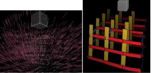
FIGURE 1.4. Two volume visualizations of the “flow” of acoustic sensor information in the tracking domain

1.4. A Stochastic Framework for Tracking System Design Optimization

Along with many dimensions to the design space, there are many possible criteria for performance of a tracking system. For example one might be concerned about resolu-tion/precision, noise, static accuracy, or dynamic accuracy. In a 6D system one might be more concerned about orientation than position, or visa-versa. See [53, 19, 4] for more specific criteria and discussion of performance. Without presupposing a particular perfor-mance metric, the framework for an intelligence amplification tool in the tracking domain should meet several requirements:

(1) Accommodate currently-known device types and update rates;

(2) Accommodate different device arrangements (e.g., on user, in environment);

(26)

(3) Accommodate and account for occlusion and interference (i.e. observability); (4) Account for growing uncertainty due to expected user motion;

(5) Avoid path and algorithm-dependent analysis;

(6) Support designer interaction with the proposed design; and (7) Calculate and effectively display estimated performance.

A few of these considerations bear further explanation. The term observability in the third point refers to the amount of information provided by the devices. It is formally described in Section 3.7.4, but it suffices to say here that different devices provide different degrees and amounts of information depending on, for example, the distance and angle between a source and sensor. The fourth point recognizes that the performance depends on the rate of information from the devices, when compared to the expected user motion. The notion of path and algorithm-dependent analysis in point five refers to the common practice of simulating the results of a particular user motion “track” through space and time, using a particular system design and tracking algorithm (see [101]).

After investigating many possible performance metrics, we decided on a stochastic ap-proach based on the asymptotic variance (uncertainty) throughout the working volume. This stochastic framework is attractive for many reasons, including meeting the above re-quirements. In particular, as described in Section 3.3, any tracking system can be consid-ered and described using state-space models. In addition, as described in Section 2.2, there are relatively well-understood methods for estimating the asymptotic (a.k.a. steady-state) performance of systems described in this form.

1.5. Hardware Information Optimization

(27)

software algorithms and motion paths as described in Section 1.5.1. In addition, the param-eters required as input to compute the system-level analysis can be evaluated and compared for optimization of the hardware devices themselves as described in Section 1.5.2. This is another contribution of the work presented in this dissertation.

Figure 1.5 shows the human-in-the-loop hardware design optimization process inserted into the traditional design sequence. Notice that it occurs before algorithm selection (i.e. it is algorithm-independent) and does not replace simulation and prototyping. Given de-scriptions of hardware devices, the desired working volume, and a model for the expected user motion, a tracking system designer can iterate through various system configurations to produce a graphical depiction of the expected position and/or orientation uncertainty throughout the working volume ofanytracking system. In this way, a designer can explore the variations between designs for a single tracking system. In addition, a designer can compare the performance of multiple systems that may use completely different physical mediums.

1.5.1. System-Level Optimization. The fundamental metric computed in the stochastic framework for hardware design optimization is steady-state covariance,P∞_{. It can be}

cal-culated before either real or simulated system measurements are available. P∞ _{is defined}

as

(1) P∞₌ _lim

t→∞

En(x(t)¯ −x(t))(ˆ x(t¯ )−x(t))ˆ To

where ¯xand ˆxrepresent thetrueandestimatedstates (position and/or rotation, for example) andEdenotes statistical expectation.

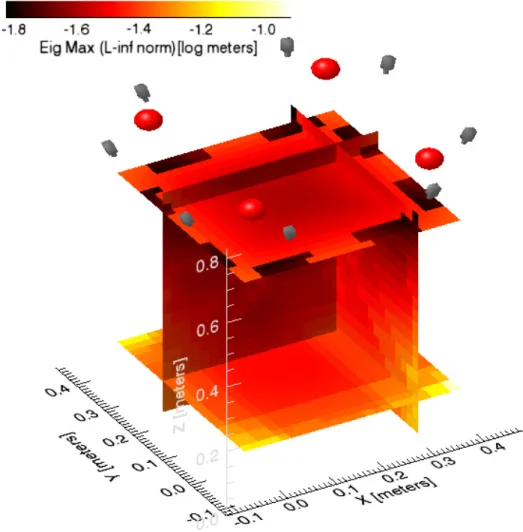
An example ofP∞ _{analysis for an acoustic tracking system is illustrated in Figure 1.4.}

The red spheres at the top of the visualization represent four speakers and performance is better (darker) near the transmitters (speakers) and towards the center of the volume where the four acoustic sensor ranges overlap and declines (lighter) in the downward direction.

(28)

FIGURE1.5. Hardware Optimization (in red) integrated into the traditional tracking system design process

Once a system has been defined and analyzed, one can alter or interact with a candidate hardware system, varying the types and configurations of devices and graphically visualiz-ing the correspondvisualiz-ing effects on the system performance. From this interaction, designers gain insight intoparticulardesign choices, as well as the relative effects of variations be-tweencandidate designs, independent of the tracking algorithm chosen for the real system and specific motion paths.

1.5.2. Measurement-Level Optimization. In addition to computing the fundamental met-ric (P∞_{) for system-level performance evaluation, the elemental building blocks of this}

(29)

motion) can be used for analysis of measurement devices. For some types of measure-ments, the quality may increase with sampling duration (i.e., averaging or correlation) but during this sampling time, a tracked target may be moving. So while the system is waiting to acquire improved measurements, it is unable to observe to the movement of the tracked target in discrete steps and may ironically see increased noise in the measurement due to the motion of the target. By examining the relationship between user motion and measure-ment behavior over time, the optimal balance between these opposing system elemeasure-ments can be determined. This measurement-level analysis is presented in Section 6.2 and is applied to a working tracking system in Section 7.3.

1.6. This Dissertation

1.6.1. Thesis Statement. Characterization of a human motion tracking system in a state-space stochastic form offers new opportunities to optimize the hardware design, indepen-dent of the estimation algorithm used in the actual system. One can employ closed-form steady-state analysis to explore and compare the expected overall performance correspond-ing to different hardware configurations. Further, one can determine the optimal sensor sampling time to maximize the filtering of random measurement noise while minimizing the impact of intra-measurement target motion.

1.6.2. Contributions.

• Establish that the stochastic framework (Chapter 3) enables complimentary

system-and measurement-level hardware information optimization, independent of algo-rithm and motion paths;

– The system-level analysis (Section 1.5.1) provides human-in-the-loop intelli-gence amplification for optimization of aggregate hardware information against expected user motion;

(30)

– The measurement-level analysis (Section 1.5.2) provides a method for opti-mization of individual measurement information against expected user mo-tion;

• Mapping of the stochastic framework to a software architecture and prototype

(Chapter 4).

• Experimental evaluation (Chapter 5) in support of verification of system-level

steady-state analysis of tracking system hardware design.

• Theoretical analysis (Chapter 6) aimed at supporting the validity of both the

system-and measurement-level optimization methods;

• Application of both the system- and measurement-level optimization methods to

a working system (Chapter 7);

– The conclusions reached in the case study analysis could improve the already high performance of the HiBall tracking system;

– The conclusions reached in the case study analysis enable reduction of the infrastructure of the HiBall tracking system;

(31)

world. In short, verification deals with mathematics and validation deals with physics (i.e., the physical world). Both qualification and validation attempt to establish the representa-tional fidelity of the conceptual (qualification) and computation (validation) models to the physical system and so qualification may be considered another form of validation [67]. Therefore, instead of QV&V, most of the literature speaks to V&V where validation may mean either conceptual or computation validation. Once a system has attained a level of validation, it can be used forprediction, the use of a computational model to foretell the state of a system under conditions for which it has not been validated [2]. Prediction is an inference based on validation evidence. Examples of the predictive capability of the framework will also be presented.

1.6.4. Nomenclature. Throughout this thesis I use lower-case variables with over-bars, hats or tildes (x, ˆx, ˜x for example) to denote a vector, and upper-case variables to denote matrices. I use the termdesigner or user to refer to the engineer or researcher evaluat-ing the system, and the termtarget to refer to the object being tracked. Example targets include a sensor on a person’s head, a retroreflective sphere on a joint or limb, and poten-tial 3D surface points that one wants to reconstruct using cameras and image/vision-based techniques.

I use a simple acoustic 3D position-tracking system to provide a concrete basis for discussion. This system is depicted in Figure 1.6, and a corresponding visualization of the estimated performance from one possible set of descriptive system parameters is shown in Figure 1.4. There are four speakers permanently mounted in the upper corners, and a microphone mounted on the moving tracking target (or user). The curve in the middle represents an example target motion path through the 3D space over time, and the point

¯

x(t)∈ℜ3represents the 3D position orstateof the target at timet.

(32)

FIGURE 1.6. A simple acoustic 3D position tracker example.

1.6.5. Structure of this Dissertation. In Figure 1.7, the AIAA QV&V model is presented on the left and a mapping to the structure of this thesis is shown on the right.

FIGURE 1.7. Phases of Modeling and Simulation: Qualification, Verifica-tion and ValidaVerifica-tion (QV&V) [2]

(33)

framework and visualize the resulting performance estimate. Typically, scientists and en-gineers speak to verification before validation. However, I will present validation before verification in order to better provide an understanding of what steady-state analysis does and a context for verification. In Chapter 5, I present experiments aimed at validating the use of asymptotic estimates and visualizations, and concrete examples of the approach used to evaluate systems. After presenting the validation results, I address the importance of ac-curate modeling parameters in Chapter 6 and apply the techniques from this chapter in a case study (Chapter 7) and predict the behavior of modified tracking systems. In Chapter 8, I discuss future plans for this research.

(34)

CHAPTER 2

Related Work

2.1. Tracking System Performance Analysis

Tracking and motion capture for interactive computer graphics have been explored for over 35 years [94, 70, 9, 66, 104] by both commercial and academic researchers who have utilized mechanical, magnetic, acoustic, inertial, and optical technologies. For example, commercial magnetic tracking systems from Ascension and Polhemus have enjoyed pop-ularity as a result of a small user-worn component, relative ease of use, and robustness for many applications. Optical systems include the HiBall-3000TMsystem by 3rdTech, the FlashPointTMand PixsysTMsystems by Image Guided Technologies, and the laserBIRDTM system by Ascension Technology. Foxlin et al. at Intersense in particular have had suc-cess developing hybrid systems that combine inertia measurements with acoustic signals [37, 38, 40], and with passive optical signals [37]. Similarly, optical systems for 3D motion capture have a long history, having been explored for over 30 years [107]. Today, compa-nies like Vicon, Motion Analysis, and Ascension make turn-key optical systems that are used in human and animal motion analysis and industrial applications. Much work has also been done on vision-based approaches to motion capture [68].

(35)

The U.S. Army Research Laboratorys Army Research Office (ARO) stated in a 2005 BAA [95] that “there are no effective methods for predicting the performance of an Image Analysis and Processing system, given the input signal or parameters of the scene such as time of day or nature of clutter”. This extends to broader category of tracking systems where, instead of or in addition to parameters such as time of day or nature of clutter, we speak of camera placement, field-of-view, occlusion, diffraction, multipath, etc. With or without these “effective methods”, tracking system researchers and commercial developers must analyze their systems and offer some measure of performance.

Since tracking systems often exhibit non-uniform performance over space, the com-mon practice of using a single set of statistics to specify a system’s global performance is inadequate and potentially misleading [39]. The engineers at Northern Digital, Inc. (NDI) contend that typical assessments are not likely to accurately reflect performance in most users’ intended environments and that a tool is needed to enable users to sample perfor-mance throughout regions of the tracking volume. To this end, NDI provides an Accuracy Assessment Kit to test the accuracy of PolarisTMpositions sensors in the field. While such tool is useful to the end-user and is a step in the right direction for analysis and assess-ment of tracking system performance, this tool is specific to a single tracking technology, algorithm and medium.

Whether predicted or assessed, performance measures vary not only in magnitude (one system is twice as accurate as another, for example) but also in modality (accuracy vs. precision metrics, for example). The ultrasonic Lincoln Wand [83] (1966) claims a posi-tional resolution of 0.02 inches and absolute accuracy of 0.2 inches. In 1974, Burton and Sutherland reported accuracy of 7.3 mm for their optical position tracker, Twinkle Box [20]. The laser-based Minnesota Scanner [88] reported accuracy of 0.04 inches RMS and 0.034 in tangential resolution in 1989. In 1999, Welch reported estimation errors of 0.2 mm at 1.9 meters and 0.5 mm at a height of approximately 1 meter for nearly all of the

(36)

working volume of the HiBall optical tracking system [103]. Polhemus advertises accu-racy and resolution of 0.03 inches RMS and 0.0002 inches per inch [78], respectively for its FASTRAKTMelectromagnetic tracking system. With the exception of the Constellation tracking system [38] in Figure 2.1, published literature about the performance of tracking systems from the first acoustic system [83] through today, typically reports performance metrics in terms of a handful of statistics that may or may not characterize the complete system performance nor permit direct comparison between tracking systems.

FIGURE2.1. Example of visualized error in the Constellation tracker [38]

(37)

Section 2.5). Further, some systems also consider the type of motion to be tracked (see Sec-tion 2.6). Within each of these secSec-tions,prediction andassessment(or some variant) will be used to distinguish between analyses that provide predictive performance estimates and those that provide performance measurements of an existing tracking system, respectively.

2.2. Qualitative Performance Analysis

Laerhoven et al. [57] instrumented a wearable harness with thirty accelerometers to assess whether system performance improves with the addition of sensors. The authors defined performance as the system’s context-awareness algorithm’s ability to distinguish between twenty defined contexts such as walking, standing, running, in a meeting, etc. Fig-ure 2.2 shows the output stream from the thirty accelerometer configuration while walking and the performance metric of context distinction (i.e., the ability to successfully discern the correct context) as the number of possible contexts are increased from 1 to 20. Note that the number of sensors increases as expected from right to left on the left axis (# sensors) but that the number of contexts decreases from left to right on the right axis (# contexts). The system performs better per this qualitative metric given the greatest number of available sensors and the fewest number of contexts from which to select (the back corner of the plot where the z-axis value is highest and largest).

Hollerer et al. [43] qualitatively assessed the accuracy of magnetic and inertial tracking systems in indoor environments by tracking users traveling along a known path (an outer hallway of their research building) and plotting the tracked path on the floor plan of the re-search building. The loop in the path on the left edge of the left image in Figure 2.3 shows the most dramatic effect of magnetic distortion from a nearby magnetic resonance imaging (MRI) device (two floors directly above) on the performance of the magnetic tracking sys-tem and the effect of “drift” on the performance of the inertial device is shown on the right. The arrows on both the left and right plots show the start and direction of the traveled track.

(38)

FIGURE2.2. Accelerometer output while walking (top) and context detec-tion performance (bottom) [57]. The vertical axis label on the bottom plot was added for clarification.

2.3. Qualitative Performance Analysis with Interaction

(39)

FIGURE 2.3. Tracking performance of magnetic (left) and inertial (right) systems [43]

cameras at will to predict system performance. It provides a realtime visualization of the mapping of camera pixels to a targeted surface for a qualitative assessment of performance as shown in Figure 2.4. With this tool, a user can locate occluded areas or, for example, determine whether the areas of interest are covered by two cameras for stereo. Further, in terms of available information, four cameras is qualitatively better than three is better than two is better than one or none. A particularly useful output of Pandora are the calibration matrices for the cameras in the scene which can be used as input for further analysis.

FIGURE 2.4. The Pandora Interactive Camera Placement and Visibility Simulator [89]

(40)

2.4. Quantitative Performance Analysis

In an environment like telesurgery, it may not be sufficient to know that the tracking system configuration in use is the best possible one. Instead, numerical performance met-rics are mandatory to show that the tracking system performance requirements are being met. Due in part to applications of this kind, methods and tools for camera placement for vision-tracking are a popular topic for both performance prediction and assessment.

Davis et al. proposed a method for designing marker-based tracking probes [30] and for predicting accuracy in pose estimation of these same type systems [29]. Using their “Viewpoints Algorithm” and a first-order error propagation to apply the errors from indi-vidual markers to overall pose estimation, an optical system using fiducials can be designed and analyzed but this approach does not extend beyond this context.

In 2000, Fleishman et al. [36] presented a predictive, automatic camera placement for image-based modeling from scenes with known geometry. Beginning with a large database of potential camera positions, they present a visibility algorithm to produce a minimal subset of camera positions that covers every visible polygon in a scene. This work draws heavily from the work presented by McMillan and Bishop [65], specifically the plenoptic function which describes all of the image information visitable from a particular viewing position.

(41)

FIGURE 2.5. Example of visualized mean radial spherical errors [73]

Olague [74] addresses the problem of minimizing error in 3D measurements for pre-dicting optimal camera placement for accurate reconstruction. A criterion using the maxi-mum eigenvalue of a computed covariance matrix is established and a global optimization process employing genetic algorithms is applied to minimize this criterion. While this approach is similar to the one presented here, it is specific to camera network design.

Livingston and State [62] created a noise metric for use in magnetic tracker calibra-tion assessment for augmented reality applicacalibra-tions within a defined working volume. After collecting sample data from both Ascension Technology’s Flock of Birds magnetic track-ing system and Faro Metrecom’s IND-1 mechanical Faro arm, they defined error metrics in terms of the local coordinate systems of the two tracking systems. For both position and orientation, the difference in either distance or quaternion angles (respectively) was calculated for multiple readings at each sample point. In both cases, the length of the di-agonal of a bounding box around the plotted errors is the noise metric. In a coincident publication, Livingston [61] presented four methods for the visualization of rotation fields

(42)

resulting from the calibration of the Flock of Birds magnetic tracking system as described above. Animated axis stream surfaces and axis streamlines were shown to be the best for highlighting heterogeneity in the rotation field and areas of large tracker error, respectively. Figure 2.6 shows position error (left) and rotation error using the axis stream surface visu-alization technique (right).

FIGURE 2.6. Visualizations of position [62] and rotation [61] error from calibration of Ascension’s Flock of Birds for use in Augmented Reality en-vironments

2.5. Quantitative Performance Analysis with Interaction

A tool developed for real-time prediction and visualization of acoustic sound fields [55] was applied to the design of the Center for New Music and Audio Technologies (CNMAT). Real-time interaction with proposed design elements such as shape of the room, position and orientation of the sound sources, microphones and audience seating aided sound en-gineers in tradeoff studies for the varied uses of the theater. Example visualizations of acoustic field behavior are shown in Figure 2.7.

(43)

FIGURE 2.7. Organ pipe sources with performer and audience cut planes (left) and time delay isosurface (right) [55]

diffuse ray–tracing along with Monte Carlo techniques to generate visualizations of acous-tic simulation. C80 (measured in decibels) is defined as the logarithmic ratio of the early arriving sound energy from 0 ms to 80 ms divided by the late sound energy arriving after 80 ms. Figure 2.8 shows a visualization of simulated sound clarity in (from left to right) fan-shaped, box-shaped and reverse-fan-shaped concert halls. The reverse fan-shape (right) has the bestC₈₀ values and the least variation in those values of the three possible concert hall shapes.

More recently, Pulkki [80] introduced Vector Base Amplitude Planning (VBAP) to create two- and three-dimensional sounds fields into which any number of virtual sound sources can be inserted interactively for predictive planning. A digital simulator that im-plements this method for up to eight loudspeakers was also developed.

2.6. Performance Analysis with User Motion

Incorporation of user motion into the analysis of tracking system performance could be the difference between an accurate simulation of performance and not. Systems that

(44)

FIGURE 2.8. Sound Clarity in (from left to right) fan-shaped, box-shaped

and reverse-fan-shaped concert halls [91]

work well in dynamic environments may not perform as effectively in static environments and vice versa. Research in the area of acoustic system performance is typically specific to quantitative acoustic behavior (as opposed to a measure of system performance quality) but must take into account the inherently dynamic environment of a concert hall for example. Godot [97] is a predictive software system for room acoustics design. Sound beams are traced as they traverse a polygonal model of a room and linear least-squares prediction is used to determine the coefficients of a digital filter that matches the frequency response of each acoustic path. From this an audible simulation of the proposed acoustic design can be generated. Unlike many point-design analysis tools, Godot II [98] accommodates moving objects (i.e. people) in a room.

(45)

drawn from a probability distribution function. While M-Track does accommodate hetero-geneous cameras (different frame rates, focal lengths, etc.), it is limited to the analysis of camera-based systems in determining optimal configurations.

FIGURE 2.9. Example of error (3D uncertainty) vs. number of cameras surrounding a sphere with and without occlusion [24]

2.7. Intelligence Amplification and Augmentation

Whether an analysis is qualitative, quantitative, interactive or sensitive to user motion, the goal is a common one. All calculate and communicate information hidden from the un-aided human. In his classic 1956 paper “Design for an Intelligence-Amplifier” [6], Ashby presented a possibility proof of a machine that would solve problems its creators were inca-pable of solving. In his 1962 report [33], Engelbart presented a conceptual framework for “augmenting human intellect”. This framework for increased intellectual capacity aimed to gain comprehension in previously overly-complex problems in order to find better solu-tions to seemingly insoluble problems faster. In both cases, the objective is not to increase native intelligence, but to augment the human being with means for organizing experience and solving problems so that an intelligent system results in which the human being is the central component [87]. The fundamental difference between Ashby’s intelligence ampli-fication and Engelhart’s intelligence augmentation is that Ashby’s intelligence-amplifier

(46)

was conceived of as a stand-alone system like the steam engine while Engelhart’s intel-ligence augmentation concept presents a system made up of a humanand the means for augmenting human intellect such as Vannevar Bush’smemex[21], a hypertext workstation that analyzes, categorizes and presents information in a comprehensive way.

(47)

CHAPTER 3

Conceptual Model: Stochastic Framework

The highlighted portion of Figure 3.1 (outlined and in red) indicates where this chapter falls in in the QV&V process. Here we map the problem domain (evaluation of human tracking systems) to the proposed stochastic representation.

FIGURE3.1. The Qualification Process

3.1. Statistical Uncertainty

(48)

stochastic estimate of the asymptotic orsteady-stateerror covariance (P∞_{) throughout the}

working volume.

3.2. Steady-state covariance

Consider the example acoustic 3D position tracking system. At a representative set of 3D points{x¯1,x¯2, . . . ,x¯p}throughout the working volume we can estimate and graphically

depict the steady-state error covariance (P∞₎

(2) P∞

i =_tlim_→

∞

En(x¯i(t)−xˆi(t))(x¯i(t)−xˆi(t))T

o

,1≤i≤ p

where ¯x_i and ˆx_i represent the true and estimated states (respectively) at point i, and E denotes statistical expectation. Note that the method does not attempt to estimate ¯x_i, ˆx_i or the residual ˜xi where ˜xi=x¯i−xˆi which would require measurements. Instead, P∞ is

estimated directly from state-space model of the system and stochastic estimates of the various noise sources.

3.3. State-Space Models

To estimate the statistical uncertainty (i.e. steady-state error covariance) of the state, we begin by mathematically describing the expected target motion and the measurements using state-space models. State-space models are essentially a notational convenience for esti-mation and control problems, developed to make what would otherwise be a notationally-intractable analysis tractable [52, 4] by representing the variables (inputs, outputs and states) as vectors and the differential and algebraic equations (dynamics) as matrices.

(49)

needed) pose derivatives. For example, a 3D-pose ( ¯x) as described above that includes position without derivatives is shown in Equation (3).

(3) x¯= [x y z]T

A 6D-pose that includes both position and orientation without derivatives is

(4) x¯= [x y z φ θ ψ]T

whereφ,θ andψ are roll, pitch and yaw euler angles (rotation around the x-, y- and z-axis)

respectively. Other rotation angle representations (such as quaternions) can also be used. An important factor in determining the appropriate state variables is the type of motion expected in the tracking environment. These motion models (Section 3.3.2), along with the measurement systems (Section 3.3.3) themselves, influence whether the state should include derivative measurements and, if so, what derivative order.

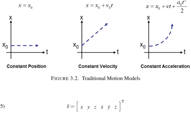
3.3.2. Motion Models. Traditionally, motion model types are described in terms of the physical parameter that is constant or uniform over time. The types of constant or uniform motions of interest [23] are constant position(CP), constant velocity (CV) and constant acceleration(CA) which displayzerovelocity, acceleration and jerk, respectively, as illus-trated in Figure 3.2.

In stochastic estimation, noise is injected into the process in place of the “zero” term so that, in the case of constant velocity motion, for example, acceleration is not zero but is instead normally-distributed random noise. Thus, position would instead be modeled as x=x₀+vt, where v=R

a, anda∼N(0,q). This is a Position-Velocity Motion Model. The state variables for a position only tracker with a PV motion-model (i.e. includes first derivatives) is shown in Equation (5).

(50)

FIGURE 3.2. Traditional Motion Models

(5) x¯=h x y z x˙ y˙ z˙ iT

Position (P), Position-Velocity (PV) and Position-Velocity-Acceleration (PVA) motion mod-els map to the traditional constant position, velocity and acceleration modmod-els, respectively. Table 3.1 shows the process of noise integration through to 1D position for each of the three stochastic motion models.

TABLE3.1. Stochastic Motion Models N(0,q)→R

→x(t) N(0,q)→R →R

→x(t) N(0,q)→R

→R →R

→x(t)

Position (P) Position-Velocity (PV) Position-Velocity-Acceleration (PVA)

These integration processes apply to 3D position, 3D orientation plus 6D position and orientation state spaces. In all cases, integration is over some time interval,δt, as described

in Section 3.3.

Each stochastic motion model corresponds to some actual target motion. For exam-ple, P-motion might be an appropriate choice for surgical environments where the surgeon moves slowly and methodically and perhaps not at all over someδt. In this case, the pose

(51)

position is modeled as a random walk. PV motion is typical of most larger-scale environ-ments in which a human target is walking or moving at a normal pace (i.e. not running or quickly changing direction) and velocity is modeled as a random walk. PVA motion is rapid and dynamic with sudden changes in speed and direction as one might observe in dancing, jumping or high-energy sports such as baseball (swinging a bat) or boxing (throw-ing punches). In this case, acceleration is modeled as a random walk and the uncertainty in pose between observations (over δt) is high. It is possible (even probable) that a

sin-gle motion type will not completely describe any sinsin-gle given activity over a non-trivial time duration. For example, a person might switch from PV-motion to P-motion if s/he stops to observe an object or activity in a virtual environment after crossing a room for a closer look. PVA-motion in humans is not maintainable over any significant length of time and can be thought of as short, even instantaneous, bursts of energy. P-motion is per-haps the easiest of the three motion model types to imagine while PV- and PVA-motion are more difficult. While not intended to serve as a rigorous proof, the following discussion should provide intuition about the different types of motion models, specifically PV- and PVA-motion models.

Carnegie Mellon University’s (CMU) Graphics Lab Motion Capture Database offers over 2600 motion trials in many categories from common behaviors such as typing on a laptop (an example of P-motion) to more dynamic activities, including sports. Trial 13 for Subject 15 [22] contains approximately 78 seconds of shadow boxing motion capture data at 120 frames per second (fps) using only the right-hand to punch initially and then switching to the left-hand alone. For approximately the first 50 seconds, right-hand punches are thrown and for the remaining 38 seconds left-hand punches are thrown. A video of the motion capture trial (30 fps) can be found at the CMU site [22] and still frames for a portion of the video are captured in Appendix B for reference. The video frame numbers (1273 through 1632) approximately correspond to seconds 42 through 54.

(52)

Figure 3.3 shows the y-axis position as captured along with the calculated velocity, ac-celeration and jerk data for the boxer’s right hand during the entire trial. The apices of the final four right-hand punches can be observed in frames 1290, 1340, 1430 and 1480. All four graphs in Figure 3.3 are repeated in Appendix A on a larger scale and with annotation. For readability and proximity, the annotations are not included in Figure 3.3. The boxer throws 28 punches as marked in Appendix A and these punches are dynamic, sometimes covering as much as 50 inches from start to finish as the boxer moves forward and back-ward with his punches. To the right of the dashed line marked “Transition to left-hand punches” the position data becomes much less dynamic as the right hand is being held up in a defensive stance as the boxer bobs and weaves, punching with his left hand. By taking derivatives of this data, we can observe PVA-motion in the boxer’s right hand when the boxer is throwing punches with his right hand and and PV-motion when he punches with his left hand.

(53)

FIGURE 3.3. Boxing Motion Capture right hand y-axis data (from top to

bottom) position, velocity, acceleration and jerk

(54)

3.3.3. Measurement Systems. The measurement system is the collection of sources and/or sensors used to observe the human in motion. Examples of commercial and research sys-tems that utilize these mediums are listed in Section 2.1 and can be classified in terms of employed medium(s), geometry, etc. The five physical mediums employed in tracking measurement systems are mechanical, magnetic, acoustic, inertial and optical. Beyond the physical medium, measurement systems can be described as inside-looking-out or outside-looking-in (sensors on the user versus sensors in the environment). System measurements can be absolute or relative (at a specific time or a change from the previous estimate), de-rivative measurements, instantaneous or averaged over time. The system can be active or passive; linear or non-linear. The geometric arrangement of the source/sensor devices is another facet of the measurement system. Each measurement system will have a unique set of parameters that calibrate and map its measurements to the mathematical framework.

3.3.4. System Dynamics. The state variables and measurements are related by a pair of differential or difference equations. One equation moves the state over time and the other maps the measurements to the state space. These two first-order stochastic equations de-scribe thesystem dynamicsas shown in Figure 3.4 where, for tracking systems, the input vectors (Cu¯_k and Du¯_k) are zero (i.e. input elements ¯u₁=u¯₂=...=u¯_n=0 so there is no controllable input), ¯z is an m-length vector of available measurements from devices such as accelerometers, gyroscopes, cameras, etc. and ¯wand ¯vare white, normally-distributed, random noise with zero-mean.

The top equation in Figure 3.4 is theprocess modeland the bottom equation is the mea-surement model. These two equations serve in some form as the basis for most stochastic estimation methods. Both models are composed of a deterministic component (matricesA andH) and a random component ( ¯wand ¯v).

(55)

FIGURE 3.4. Block diagram of a linear stochastic dynamic system in

dis-crete time (based on a Figure in [42]). Both ¯u_k vectors are zeroed because there is no controllable input.

(6) xˆ_k₊₁=Axˆ_k+w¯_k

where ¯w∼ N(0,Q). The corresponding (continuous-time) differential equation can be modeled as shown in Equation (7).

(7) x(t˙ ) =A_cx(t) +q_c(t)

where A andAc are n×ndiscrete- and continuous-time state transition matrices,

respec-tively.

The measurement system is described by an equation that maps measurement-space to state-space. It is common to model them-dimensional device measurements ¯zat discrete timekas

(8) z¯_k=Hxˆ_k+v¯_k

(56)

where H is an m×n matrix relating the n-dimensional state to the m-dimensional mea-surements, and ¯v(like ¯w) represents zero-mean, white measurement noise, presumed to be uncorrelated with ¯w.

In practice the actual noise signals ¯w and ¯v are not known or estimated as part of a stochastic estimator. Instead, designers typically compute the process and measurements as

ˆ

x_k = Axˆ_k₋₁, (9)

ˆ

z_k = H_kxˆ_k, (10)

then estimate the process and measurement noise covariances Q and R of the presumed normal distributions ¯w∼N(0,Q)and ¯v∼N(0,R), and use those covariances to weight the measurements and to estimate the state uncertainty. It is the deterministic parameters, A andH, and the random parameters, Qand R, that the designer must specify to perform a steady-state analysis.

3.4. Non-Linear State-Space Models

In cases where the process and/or measurement models are non-linear, equations (9) and (10) would be written as shown in Equation (11) and Equation (12).

ˆ

x(t) = f(x(tˆ −δt))

(11)

ˆ

z(t) = h(x(t))ˆ (12)

(57)

A = ∂

∂x¯f(x)ˆ

¯ x (13)

H = ∂

∂xˆh(x)ˆ

ˆ x (14)

and use them in place of their corresponding matrices in equations (9) and (10). While such linearizations can lead to sub-optimal results (Section 6.1.1), they provide a computation-ally efficient means for estimation, and in most cases should offer a reasonable basis for comparison of steady-state results. For linear models, the designer would write functions that implementAandH (linear functions in matrix form) from equations (9) and (10). For non-linear models, the designer would instead write functions that implement the respective Jacobians from equations (13) and (14). Note that the Jacobians resulting from equations (13) and (14) will also be correct for linear models as well, resulting in equations 9) and (10. An alternative to the non-linear (aka Extended) Jacobian equations is the Unscented filter approach [48].

3.4.1. Process Model. In the discrete-time process model described by Equation (6), the state transition matrix A moves the target’s state forward over some interval of time, δt.

The termAx¯models the deterministic portion of the process, while the term ¯w and corre-sponding covarianceQmodel the random portion of the target’s motion.

To start, let’s examine a simple 1D position tracking system with derivatives such that the state is defined as ¯x= [x x]˙T. To move the estimated state vector ˆx_k forward in time

δt, the new position ˆxk+1is a function of the previous value ˆxk, the corresponding velocity

element ˆ˙x, and the timek δt since the last update as shown in Equation (15). The velocity

element ( ˆ˙x) does not change as shown in Equation (16).

(58)

ˆ

x_k₊₁ = xˆ_k+xˆ˙_kδt

(15)

ˆ˙

x_k₊₁ = xˆ˙ (16)

Putting these equations into matrix form,

A=   1 0 0 1  

where A is the deterministic portion of the discrete-time process model given in Equa-tion (9).

It is in determining the random component (Q) of the process model that Equation (7) becomes important. The discrete-time (sampled) Q is a function of the continuous-time process components,A_c andQ_c, andδtsuch that

(17) Q=

Z δt

0

eAct_Q

ceA

T ct_dt

as described in [42]. The continuous-time process noise is ann×1 vector such thatq_c = [0, ...,0,N(0,q)]T with correspondingn×nnoise covariance matrixQc=E{qc,qTc}.

Putting these equations into matrix form, we haveA_candQ_c as shown below.

Ac=

 

0 1 0 0



 and Qc=

  0 0 0 q  

For completeness, Table 3.2 shows the continuous-time process parameters correspond-ing to P, PV and PVA motion models [99].