M
ODELINGH
ETEROGENEOUSP
EERA
SSORTMENTE
FFECTS USINGL
ATENTC
LASSP
SEUDO-M
AXIMUML
IKELIHOODE
XPONENTIALR
ANDOMG
RAPHM
ODELSTeague R. Henry
A thesis submitted to the faculty of the University of North Carolina at Chapel Hill in partial fulfillment of the requirements for the degree of Master of Arts in the Department
of Psychology and Neuroscience.
Chapel Hill 2015
Approved by:
Kathleen Gates
Daniel Bauer
c
2015
ABSTRACT
TEAGUE R. HENRY: Modeling Heterogeneous Peer Assortment Effects using Latent Class Pseudo-Maximum Likelihood Exponential Random Graph Models.
(Under the direction of Kathleen Gates)
This thesis develops a class of models for inference on networks called Sender/Receiver
Latent Class Exponential Random Graph Models (SRLCERGMs). This class of models
extends the existing Exponential Random Graph Modeling framework to allow analysts to
model unobserved heterogeneity in the effects of nodal covariates and network features.
Simulations across a variety of conditions are presented to evaluate the performance of this
technique, and an empirical example regarding substance use among adolescents is also
presented. Implications for the analysis of social networks in psychological science are
ACKNOWLEDGMENTS
Kathleen Gates, whose advising and assistance was invaluable. Daniel Bauer and Peter
Mucha, whose comments made this thesis significantly stronger. My colleagues in the
Gates Lab, who were always willing to chat. The Quantitative Psychology program at
TABLE OF CONTENTS
LIST OF TABLES . . . viii
1 INTRODUCTION . . . 1
1.1 Network Terminology and Model Description . . . 5
1.2 A Brief Description of Exponential Random Graph Models . . . 7
1.3 Exponential Random Graph Models . . . 10
1.3.1 Structural Statistics . . . 10
1.3.2 Nodal Attribute Terms . . . 12
1.4 Estimation for ERGMs . . . 12
1.4.1 Maximum Pseudolikelihood Estimation of ERGMs . . . 14
1.5 Sender/Receiver Latent Class ERGMs . . . 16
1.5.1 Latent Class Generalized Linear Models . . . 16
1.5.2 Expectation Step . . . 17
1.5.3 Maximization Step . . . 19
1.5.4 A Note on Standard Errors . . . 19
1.5.5 Estimation for Sender/Receiver Latent Class ERGMs . . . 20
2 SIMULATIONS . . . 21
2.1 Methods . . . 21
2.2 Simulation Results for Heterogeneous Models . . . 24
3 EMPIRICAL STUDY . . . 41
3.1 Data Characteristics and Measures . . . 42
3.1.1 Measures . . . 42
3.1.2 Missing Data . . . 43
3.1.3 Model Specification . . . 44
3.2 Results of the Empirical Analysis. . . 45
4 DISCUSSION . . . 48
LIST OF TABLES
2.1 Simulation Conditions: Values are the data generating parameters per con-dition. . . 23
2.2 Mean Estimated Parameters calculated across 500 trials in each condition . 25
2.3 Mean Rand Indices and Adjusted Rand Indices (Standard Deviations com-puted from the sample) comcom-puted across 500 trials within each condition. Re-sults indicate best recovery occurs in the + conditions, with higher class sepa-ration. Structural effects such as GWESP are also recovered well. . . 26
2.4 Relative Bias in the Parameter Estimates For Heterogeneous Models, cal-culated using Mean Raw Bias over True Parameter Value. Results indicate modest levels of bias in homogeneous parameters. This bias is in line with expected bias from the approximate MLE estimation . . . 28
2.5 Mean Raw Bias in the Parameter Estimates for Heterogeneous Models, calculated across 500 trials in each condition . . . 30
2.6 Mean Estimated Standard Error calculated across 500 trials per condition
| Simulation Error calculated from the difference between the parameter esti-mates and the true parameter estiesti-mates across 500 trials per condition - Hetero-geneous Networks. Results indicate disagreement between estimated standard error and simulation error due to the implementation of classification likeli-hood estimation. . . 32
2.7 Mean Posterior Class Probabilities For True Class Assignment for both correctly classified and incorrectly classified nodes (Standard Deviation), cal-culated over 500 trials for each condition. Results indicate that when nodes are correctly classified, they have a high probability of being in the correct class. When nodes are incorrectly classified, the probability of being in the correct class is substantially lower than .5. . . 33
2.8 Mean Parameters for Homogeneous Models calculated across 500 trials for each condition . . . 35
2.9 Relative Bias for Homogeneous Models calculated with Mean Raw Bias (Table 2.10) over True Parameter Values. Results indicate that there is a sub-stantial and systematic pattern of bias in the homogeneous parameters when heterogeneity is not properly modeled. . . 36
2.11 Mean Standard Errors averaged across 500 trials per condition | Standard Deviations of the Estimated Parameters calculated across 500 trials per condi-tion for Homogeneous Models. Results indicate that there is close agreement between the estimated errors and the simulation errors. . . 40
3.1 Demographic and Descriptive Statistics . . . 42
1 INTRODUCTION
Network methods have emerged as an increasingly prominent tool in both
psychologi-cal science and the broader social sciences. For example, recent research in adolescent
de-velopment, behavior, and health utilize network methods to study the association between
peers and a variety of behaviors such as adolescent alcohol use and smoking (Osgood,
Ra-gan & Wallace, 2013; Mercken, Steglich, Sinclair & Holliday, 2012), childhood obesity
(Shin, Valente, Riggs & Hu, 2014), deviant behavior (Osgood, Feinberg & Ragan, 2015),
and sexual behavior (Ali & Dwyer, 2011). Any behavior or trait of interest to researchers
that is associated with a social network structure is likely the result of two processes,
in-fluence processes, where the network structure (who is connected with whom) changes the
behavior or trait of an individual over time and the reverse, selection processes, where the
behavior or trait changes the network structure over time. These two processes are
inter-related and together impact both network structure and the individual processes within the
network such that, over time both processes can drive dynamic, multi-level shifts. Given
this synergy between influence and selection processes, and their joint implications for
change over time, network data analysis poses a variety of complex methodological
prob-lems.
However, in recent years, new methodologies have been developed to either
simulta-neously analyze peer selection and influence processes (e.g., SIENA; Snijders, de Bunt, &
Steglich 2010), or focus on one, such as peer selection processes (e.g., STERGMs,
Kriv-itsky & Handcock, 2014). Of additional interest is peer assortment, that is, the
cross-sectional pattern of peer nominations which are conditioned upon individual traits and
and peer selection (Kandel, 1978), it provides greater insight into the nature of a given
net-work structure at any time-point. Additionally, models that investigate cross-sectional peer
assortment are similar to models that assess peer selection processes, specifically the
ex-ponential random graph modeling framework (ERGM; Frank & Strauss, 1986; Wasserman
& Pattison, 1996; Moriss, Handcock & Hunter 2008), and its longitudinal extension, the
separable temporal exponential random graph modeling framework (STERGM; Krivitsky
& Handcock, 2014).
What underlies all of these network analytic methods is their ability to assess the
ef-fect of individual level traits and covariates, such as personality characteristics or observed
behaviors, on the network structure. Furthermore, in directed networks (i.e. networks in
which edges have a beginning and end point; e.g., peer friendship networks where
indi-viduals nominate peers as friends), researchers can assess sender and receiver effects of
covariates. These effects assess the impact of a behavior, such as substance use, on the
ten-dency for individuals to send or receive edges. Breaking apart covariate effects into sender
and receiver components may prove useful when investigating the impact of individuals
behaviors on network structure (i.e., selection processes).
Parallel to network methods recent flourishing in the psychological and social sciences,
methods that seek to model and capture individual (or ideographic) differences are also
resurging and may benefit from a network approach. Modeling ideographic differences can
be done a variety of different ways, depending on the research question at hand and also
the research design. For example, an ideographic analysis of relations of effects (Molenaar,
2004) allows researchers to examine a single individuals pattern of behavior, while other
methods test the aggregate relations between outcomes as moderated by some individual
trait or other behavior (Bauer, 2011). Of the existing individual differences methods,
mod-eration by an observed variable is by far the most commonly used (Bauer, 2011). When
typical statistical techniques used. However, current methods that analyze whole networks
can also model observed variable moderators, typically through a multiplicative interaction
effect. As such, further work that focuses on improving cross-sectional and selection
net-work processes may be valuable for ideographic research, as these netnet-work methods would
allow researchers to examine individual differences in social structure and effects.
This is even more vital, given that failure to model individual differences based on
observed or unobserved variables can be significantly detrimental to researchers confidence
in the validity of their data . For example, neglecting to include moderation effects in
non-network data may result in biased estimates (Jaccard & Turrisi, 2003) and even spurious
random effects (Bauer & Cai, 2009) It follows that in network analysis, failure to account
for heterogeneity could have potentially severe consequences, especially because certain
parameter combinations can cause the estimation to converge on a degenerate solution
(Chatterjee & Diaconis, 2013). This risk of degeneracy is increased when estimating a
mis-specified model, such as the failure to account for individual differences in effects.
Given burgeoning interests in networks and individual differences, a growing number
of researchers are seeking to examine the role of moderators and individual differences
in networks. For example, in adolescent peer influence work, researchers focus on peer
selection and peer influence processes, and on how individual differences in traits and
be-haviors can shape network structure as a whole. Within this body of literature, the greatest
amount of research has examined peer influence processes (for review see, Brechwald &
Prinstein, 2011), with little work exploring potential moderators of peer selection or peer
assortment (with exception; see Kiuru et al., 2010) Furthermore, there have been no
stud-ies that have used a whole network analysis method such as exponential random graph
modeling or SIENA (Snijders, de Bunt, & Steglich, 2010) to study the moderation of peer
influence, selection, or assortment by individual characteristics. However, this paucity of
testing network-based moderation effects in peer selection or peer influence do not allow
for moderation in the estimates of behavioral or endogenous effects on network structure
that is based on unobserved or latent variables.
Latent class models and mixture models are also commonly used in psychological
re-search to assess individual differences based on unobserved data, and thus may provide
a solution to this methodological hindrance. Specifically, finite mixture linear regression
(DeSarbo & Cron, 1988) and finite mixture general linear regression (Wedel & DeSarbo,
1995) can be used to partition a sample into groups, in which each group has different
re-lations among observed variables. This potentially models individual differences that are
not due to an observed variable. One advantage to using a finite mixture regression
ap-proach in the presence of unobserved individual differences is that the regression models
for each mixture component can be a combination of component-specific parameters as
well as general parameters for which no individual differences are proposed.
In network modeling, latent variables and mixtures are commonly defined as latent
communities, or groups of individual entities (be they humans, neurons, etc.) who tend
to nominate each other more than they nominate entities in other groups. A great deal
of methodology has been developed in the last decade to assess latent community
struc-tures, chief of which are heuristic algorithms that partition networks (for review, see
For-tunato, 2010). There are several statistical methods for detecting latent communities, such
as stochastic block modeling (Nowicki & Snijders, 2001), latent space modeling (Hoff,
Raftery & Handcock, 2002), and more recently, the ERGM approach (Schweinberger &
Hancock, 2014); however, all of these approaches focus on assessing latent community
structure and do not focus on assessing individual differences in the effects of covariates
By contrast, the present thesis aims to extend the definition of latent classes and
mix-tures on networks, and model latent classes of individuals who differ in their effect of
ob-served variables on their position in the network. To accomplish this, this thesis develops a
sender/receiver finite mixture modeling approach for ERGMs, focusing on cross-sectional
or peer assortment models. This work will help address the methodological conundrum
fac-ing researchers who wish to utilize a whole network analysis method to test the moderation
of peer influence, selection, or assortment by individual differences. ERGMs are a class of
exponential family inferential models that allow the modeling of the effect of covariates on
network structure, as well as modeling the complex dependencies in networks. The form
of an ERGM makes it amenable to a mixture modeling approach. A set of simulations will
be presented that demonstrate the sender/receiver finite mixture ERGMs ability to recover
the mixture components, as well as the consequences of failing to model the individual
differences. Finally, an empirical example examining individual differences in the effect of
alcohol use on the network structure in a middle-school will be presented.
1.1 Network Terminology and Model Description
In order to work with networks as a data structure, the terminology used to describe
networks in this thesis needs to be established.
A network consists of a set ofnodesand a set ofedgesthat connect the nodes together.
Nodes define the members of a network, and can represent anything that has relations with
other things. Nodes commonly represent individuals, corporations, townships, network
routers, and brain regions of interest (ROIs). Edges define the relationship between nodes
in the network, such as friendships, board interlock, information exchange, or functional
connections. Edges can be directed (e.g., friendship nominations among adolescents) or
undirected(e.g., board interlock among companies). To store edges, and to represent them
in a fashion that amenable to analysis, anadjacency matrixis used. An adjacency matrix,A,
iandj for allN individuals.
This data structure allows the analyst to represent any network structure, be it directed
or undirected, weighted or un-weighted in a portable fashion. A directed edge Aij is the
relationship from nodeito nodej, and does not inform on the relationship from nodej to
nodei. An example of an directed edge would be a friendship nomination. The
nomina-tion of friendship from individual ito individual j does not necessitate the nomination of
friendship from individualito individualj. Other networks have undirected edges, where
Aij = Aji. One common example of this is the correlation network between regions of
interest (ROI) in the brain. A correlation is a bi-directional effect, and the corresponding
edge between ROIiand ROIjwill have the same value from regardless of the direction of
the edge.
Friendship nominations and brain ROI correlations also provide examples as to
differ-ing types of edges. The edges corresponddiffer-ing to friendship nominations take on the value
of 0, for no friendship nomination, or 1 for a friendship nomination. This type of edge
is referred to as binary. Binary networks reflect the presence or absence of a connection
between nodes. The brain ROI correlations take on any value between -1 and 1. These
connections are referred to asweightededges. The edges in a weighted network can take
on any real number value.
In addition to the presence or absence of edges, and possible weights on edges, often
timesnode-level attributesare also included in the analysis. Node level attributes are
sim-ply values that reference particular nodes. Gender is a node level value for a adolescent
friendship network, while size of an ROI is a node level variable for a brain ROI
correla-tion network. In this manuscript, theN ×P matrix of node level variables will be denoted
usingX.
The present thesis focuses on directed, binary graphs that take into account node-level
1.2 A Brief Description of Exponential Random Graph Models
Exponential Random Graph Models (ERGMs; Wasserman & Pattison, 1996) are a
fam-ily of models used to analyze network structure both contingent on endogenous predictors
as well as on covariates of the individual nodes. ERGMs model the entire network as a
sample from a population of networks with a set of sufficient statistics associated with the
population. These sufficient statistics can include the number of edges in the network,
the number of edges between individuals with dissimilar values on one specific covariate
and/or the number of closed triangles in the network, to name a few examples. These
mod-els were originally developed to analyze dyad independentnetworks, where the probability
of an edge between two nodes was only dependent on the characteristics of those two nodes
(Holland & Leinhardt, 1981). They were extended by Frank and Strauss (1986) to include
transitivity effects, where the probability of an edge existing depends on the existence of
neighboring edges.
The modeling of transitivity proves to be difficult, and only in recent years has there
been estimation procedures developed to successfully model transitivity (Hunter &
Hand-cock, 2006). Since the development of a efficient estimation procedure, ERGMs have been
actively researched in several fields, and have been extended in a variety of ways. A
longi-tudinal extension was recently developed (STERGMs; Krivitsky & Handcock, 2014) that
model the formation and dissolution of ties over multiple observations of a network.
Ad-ditionally, there has been work on modeling latent community structures within ERGMs.
Schweinberger and Handcock (2015) developed a Bayesian procedure for analyzing very
large networks, something that ERGMs typically struggle with. They succeed by modeling
a large network as a mixture of smaller sub-networks.
Increasingly in the past decade, methodology to model heterogeneity and individual
dif-ferences in networks has been under development. Heterogeneity in networks is commonly
is a type of individual difference as different nodes (individuals) are following different
rules regarding association. However, it is an overly restrictive form of heterogeneity, as
it doesn’t allow for nodes to have behave differentlyandnot group into community
struc-tures. Instead, a broader definition of a heterogeneity in network structure will be used in
this manuscript, that is a network is heterogeneous if the nodes that make up the network
behave differentially.
There are two dominant statistical methods for analyzing latent classes as latent
com-munities in random networks. Those are the Latent Space Model (Hoff, Raftery &
Hand-cock, 2002) and the Stochastic Block Modeling framework of (Nowicki & Snijders, 2001).
The latent space model posits that every node is located in a latent social space, and the
nodes connectivity to other nodes is dependent on the location of each node in the social
space. This method can be used to find community structure and implicitly accounts for
transitivity and the effects of covariates, however does not allow any heterogeneity in the
effects of the covariates on network structure.
The stochastic block modeling framework posits that a network structure is entirely
due to the latent community structure, and if the latent community structure is known, then
the edges within the network are dyad independent given community assignment.
Further-more, this framework models the network as a mixture of Erd˝os-R´enyi graphs (Erd˝os &
R´enyi, 1961) (networks where each edge is distributed i.i.d Bernoulli), which is a even
more restrictive assumption than dyadic independence. This framework has been extended
in recent years most notably with the work of Daudin (2008), where the authors develop
a mixture model on random graphs that allow for community structure to be defined in
several different ways.
In this thesis, we use the exponential random graph modeling framework to construct
latent class models. Exponential random graph models are a model based inferential system
actor based modeling (Snijders, de Bunt & Steglich, 2010) is primarily used for
longitudi-nal data, and relies on agent based simulation for estimation. Due to these properties, the
focus of development will be on exponential random graph models.
As a model based inferential system, ERGMs require the analyst to specify which
ef-fects they want to model. This provides fine grained control to the analyst, however, the
price is that these effects are homogeneous across all nodes in the network, in that
ev-ery node given the nodal covariates behaves the same. It is fairly apparent that real-data
networks are not completely homogeneous, given the recent interest in latent community
detection and other methods that explicitly assess for heterogeneity within a network. This
interest suggests that a model that allows for heterogeneities and individual differences in
ERG modeling would be of great assistance. Although it is fairly simple to model
moder-ation between observed variables using multiplicative interactions in ERG modeling, there
has been no methodology to date that allows for the modeling of latent category
mod-eration, in which the nodes in a network are partitioned into a set of latent classes, and
each class potentially has a different effect of nodal covariates and network features. This
modeling of unobserved heterogeneity is similar to the approach taken in finite mixture
regression (Wedel & de Sarbo, 1995)
The model that is developed in this thesis is termed a Sender/Receiver Latent Class
ERGM. This class of models posits that every node has a latent class assignment, and this
latent class assignment moderates the effect of specific nodal covariates on the probability
of edges directed towards the node (A Receiver Latent Class ERGM), or edges directed
away from the node (A Sender Latent Class ERGM), but not both. This division often
aligns with hypotheses made by researchers who are interested in associations between
nodal attributes and nominations. The choice to restrict the model to either assess the effect
of either sender latent class or receiver latent class was made to render the model tractable
1967; Dempster, Rubin & Laird, 1977) for reasons elaborated below.
In what follows, ERGMs and the Sender/Receiver Latent Class ERGMs will be
ex-plained in technical detail.
1.3 Exponential Random Graph Models
An exponential random graph model models the observed network as a sample from
a exponential family distribution with the following form. Let A be a random directed network of sizeN with sample spaceA, andXaN ×P matrix of fixed and known nodal covariates, withabeing a sample realization ofA. Then the distribution ofAis
P(A=a|X) = exp[hθ, s(a,X)i]
ψ(θ) (1.1)
Whereθis adlength vector of natural parameters in log-odds metric,s(a,X)is adlength vector of sufficient statistics,hθ, s(a,X)iis the inner product of the vector of natural pa-rameters and the vector of sufficient statistics and ψ(θ) is a normalizing constant. The log-likelihood of the parameters (Hunter & Handcock, 2006) is then:
`(θ) = hθ, s(a,X)i −log(ψ(θ)) (1.2)
As was outlined above, the vector of sufficient statistics s(a,X)can contain a variety of terms. Sufficient statistics that will be used in the simulation studies and the empirical
examples are described below. Broadly, these can be divided into two categories, sufficient
statistics that are wholly based on the network structure, structural statistics, and statistics
that are based on the node level attributes, node level attribute statistics.
1.3.1 Structural Statistics
What follows are the technical definitions as defined in the statistical literature.
Edges. The parameter estimate associated with the edges statistic in any ERGM acts as
number of edges in the network.
Mutuality. This sufficient statistic is used when modeling directed networks, and the
sufficient statistic is the total number of reciprocated dyads (Holland & Leinhart, 1981).
These are dyads whereaij = aji = 1. The parameter associated with this statistic can be
described as the tendency for edges to be reciprocated.
Geometrically Weighted Edgewise Shared Partners (GWESP). This sufficient statistic
is used to account for transitivity in the network (Hunter, Goodreau & Handcock, 2008).
Transitivity is the phenomena where an edge is more likely to be present if the edge has
shared partners. This is commonly referred to colloquially as ”A friend of a friend is
my friend.” Transitivity is a common phenomena in real-world networks, and failure to
model transitivity can result in bias in the estimates of other effects (Van Duijn, Gile, &
Handcock, 2009). However, when a term that models transitivity is added, this induces a
dependency structure in the network that prevents a direct maximization of the likelihood
during estimation. This dependency structure also runs the risk of causing degeneracy in
estimation, where the expected value of the networks distribution converges to a completely
empty or completely full network. Details of why this occurs can be found in Chatterjee
and Diaconis (2014). The geometrically weighted edgewise shared partners term works
to prevent degeneracy by down-weighting large numbers of shared partners. A GWESP
term has both an effect parameterθ(GW ESP) and a weight parameter τ. τ ranges from 0
to∞, with 0 meaning that the effect of shared partners does not increase beyond having 1
shared partner, and ∞meaning that the effect of additional shared partners is linear with
no asymptote.
Ifτ is allowed to be freely estimated, then the ERGM becomes a member of a curved
exponential family (Efron, 1978), which complicates estimation. In the simulations that
where the curved exponential family models fail to estimate. (Hunter, Goodreau &
Hand-cock, 2008)
1.3.2 Nodal Attribute Terms
All terms below are described in Pattison and Robins (2001).
Attribute Matching. The parameter estimate associated with this sufficient statistic is
used to evaluate the effect of nodes matching on a categorical variable such as gender or
ethnicity. The sufficient statistic is the number of edges between nodes that match on the
categorical variable.
Attribute Outdegree The parameter estimate associated with this sufficient statistic is
used to evaluate the effect of a continuous variable on the number of edges coming out
of nodes. The node level sufficient statistic is the outdegree of a node multiplied by the
attribute value for that node.
Attribute Indegree Similarly to the Attribute Outdegree term, the parameter estimate
associated with this sufficient statistic reflects the effect of a continuous variable on the
number of edges nodes in the network receive. The node level sufficient statistic is indegree
of the node multiplied by the attribute value for that node.
Attribute Absolute Difference The parameter associated with this sufficient statistic
evaluates the effect of similarity on a continuous variable between nodes on the
proba-bility of an edge. The edge level sufficient statistic is the absolute difference in the values
of the attribute for the sender and receiver of the edge multiplied by the presence or absence
of that edge.
1.4 Estimation for ERGMs
Estimation of the parameter vectorθfor an ERGM model is complicated when a term
that measures transitivity is included in the model. ERGMs, as originally proposed by
Holland and Leinhardt (1981), did not contain transitivity terms, and instead were
where the state of a dyad (what edges in a dyad are active), are conditionally independent
of all other dyads given the characteristics of the nodes that make up the dyad in question.
This simplifies the likelihood of adyad independentERGM to that of a multinomial
regres-sion for a directed network (the categories being the 4 possible states of a directed dyad),
or a binary logistic regression for an undirected network, which in turn makes estimation
of adyad independentERGM trivial.
However, when a term that accounts for transitivity, such as a GWESP term, is added to
the model the resulting dependency structure changes the likelihood into something that is
less tractable to estimation. The core of the problem with transitivity assessing ERGMs was
first realized by Frank and Strauss (1986) and stems from the definition of the normalizing
constantψ(θ). In a general ERGM,ψ(θ)is defined as such:
ψ(θ) = X
a∈A
exp[hθ, s(a,X)i] (1.3)
WhereAis the sample space of the distribution of the random graphA. This sum over
all networks of a given size is intractable for any reasonable sized network. For
exam-ple, the number of possible directed networks of 25 nodes is 2252−25 1 or approximately
4.4∗10180. Iterating over this number of networks in a reasonable time frame is impossible for any computing system currently in existence. An approximate solution to this
estima-tion problem was proposed by Hunter and Handcock (2006), which uses Markov Chain
Monte Carlo sampling to obtain a sample of networks at a given set of parameters, and
then maximize the likelihood of the parameter values using that sample to approximate the
normalizing constant. This procedure, when applied iteratively, converges to the maximum
likelihood estimates of the parameters θ as the number of iterations approach ∞. There
1 For a directed network of size N, each node has a possible number of edges equal to N-1, as self edges are not allowed. As such, the maximum number of edges in a directed network of size N isN∗(N−1)or
are several problems with this sampler, most notable of which is the difficulty in getting a
sample of networks that properly covers the density of the distribution for approximating
the normalizing constant. Estimation for ERGMs is an ongoing field of research.
Due to the iterative nature of the approximate ML estimator of Hunter and Handcock
(2006), it is less than ideal to implement in an Expectation Maximization framework, which
in of itself is iterative. Additionally, the MCMC sampler does not scale well to larger
networks, limiting the practical size of a network to less than 300 nodes. An alternative
to the ML estimator appears in the maximum pseudolikelihood approach of Frank and
Strauss (1986). Very recently there was a deterministic approximation to the normalizing
constant that operates in quadratic time, which is promising for estimating ERGMs on
larger networks (Pu et al., 2015).
1.4.1 Maximum Pseudolikelihood Estimation of ERGMs
When transitivity terms were first introduced by Frank and Strauss (1986), the estimator
proposed for ERGMs was a pseudo likelihood approach first inspired by Besag (1974)
pseudolikelihood approach for spatial models.
Recall that the distribution of observed variable ERGM is:
P(A=a|X) = exp[hθ, s(a,X)i]
ψ(θ) (1.1)
Consider now the conditional probability of an edge Aij given the rest of the network, Ac
ij:
P(Aij = 1|Acij =a c ij) =
exp(hθ,siji)
1 + exp(hθ,siji)
(1.4)
Where sij is the change in the sufficient statistics when Aij goes from 0 to 1. This
expression is identical to a logistic regression model treating the sij as fixed and known
covariates. The pseudo-likelihood approximation to the log-likelihood as developed by
of the following form:
P(A=a|θ)≈ Y
(i,j)∈a
(exp(hθ,siji))aij
1 + exp(hθ,siji)
(1.5)
Taking the log of the above transforms it to the pseudo-log-likelihood which can be
simplified as shown:
ˆ
`(θ) = log
Y
(i,j)∈a
(exp(hθ,siji))aij
1 + exp(hθ,siji)
= log
"
exp(P
(i,j):aij=1hθ,siji) Q
(i,j)∈a1 + exp(hθ,siji)
#
= X
(i,j):aij=1
hθ,siji −
X
(i,j)∈a
log(1 + exp(hθ,siji)
Note that hθ, s(a,X)i is equal to P(k)
θ(k)s(k)(a,X), and that s(k)(a,X) is equal to
P
(i,j):aij=1s
(k)
ij . Therefore
P
(i,j):aij=1hθ,siji = hθ, s(a,X)i. This leads to the final
ex-pression of the pseudo-log-likelihood below:
ˆ
`(θ) = X
(i,j)∈a
log(P(Aij = 1|Acij)) =hθ, s(a,X)i −
X
(i,j)∈a
log(1 + exp(hθ,siji)) (1.6)
Note that this pseudo-log-likelihood differs from the log-likelihood only in the
normal-izing constant. This pseudo-log-likelihood is identical to that of a binary logistic regression,
and can be maximized by established means.
There are several issues with using the MPLE for ERGMs that model transitivity.
Lub-bers and Snijders (2007) provide evidence that the standard errors of the estimates in an
MPL fit ERGM tend to be underestimated, and the whole model tends to overfit to the data.
transitivity parameter from an MPL fit ERGM are substantially less efficient than that of
a ML fit ERGM. However, recently it has been proposed that the properties of the MPL
estimator have not been thoroughly studied (Chatterjee & Diaconis, 2013), and that there
is evidence for its asymptotic normality (Comets & Janzura, 1998).
Although it is entirely possible to use MLE when obtaining latent class solutions, there
are several issues that suggest MPLE is a better choice for estimation. As will be shown,
the latent class solution for a sender/receiver latent class ERGM is estimated using the
EM algorithm. Using the MLE during the maximization step is computationally intensive,
with running times an order of magnitude above the running time of MPLE. Furthermore,
in light of the possibility of degeneration, repeated applications of the MLE while using
non-optimal latent class solutions increases the probability that at least one iteration will
be degenerate, which would cause estimation to fail. As such, in current thesis, we use
MPLE during the maximization step of an EM algorithm implementation. Given the known
issues with MPLE, we use MLE to obtain a final set of parameter estimates, once the EM
algorithm has converged.
1.5 Sender/Receiver Latent Class ERGMs
1.5.1 Latent Class Generalized Linear Models
In 1988, Wedel and Desarbo developed a mixture model for generalized linear models.
This approach relies on the hard EM type algorithm for estimation, otherwise known as
the k-means algorithm (MacQueen 1967, Dempter, Rubin & Laird, 1977), and provides an
elegant solution to the estimation problem in this thesis. As the MPL for an exponential
random graph model is identical to the likelihood for a binary logistic regression, Wedel
and Desarbo’s approach can be applied.
The joint log pseudolikelihood for a Sender Latent Class ERGM as derived for the first
ˆ
`(Z,θ) =X
i Q
X
q=1
Ziqlog(αq)+
X i X j6=i " aij " Q X q=1
Ziqhθq, siji
#
−
Q
X
q=1
Ziqlog(1 + exp(hθq,siji))
#
(1.7)
Where Ziq is 1 if nodei is in class q and 0 otherwise. αq is the marginal probability
of a node being in classq. θq is a vector of parameters for classq. aij is the value (0 or 1
for a binary network) of the edge from nodeito nodej. sij is the vector of changes in the
sufficient statistics of the network if edgeaij went from 0 to 1, given the rest of the network.
Any parameterθmay be held equal across all classes, and thus rendered homogeneous.
1.5.2 Expectation Step
The general expectation for a latent class general linear model (where the probability
densities are exponential family) is in the following form (Wedel & DeSarbo, 1995, Eq 7):
E[ziq|θ,yi] =
αqQKk=1fik|q(yik|θq)
PQ
q=1αq
QK
k=1fik|q(yik|θq)
(1.8)
Whereyiis a vector of observations (each of which can come from a different arbitrary
probability density) for case i and fik|q(.) is the probability density function for the kth
element of theith case given theith case is in classq.
Here we can express the expectation for the sender latent class exponential random
graph model in precisely that form of Equation 1.8.
E[ziq|θ,a] =
αqexp(Pj6=i[aij[hθq, siji]−log(1 + exp(hθq, siji))])
PQ
q=1αqexp(
P
j6=i[aij[hθq, siji]−log(1 + exp(hθq, siji))])
(1.9)
Note that in the above likelihood, edges that share the same sender node all are assigned
the same latent class. Intuitively, this is due to the assignment of the latent class being
as they classify observation vectors. In this case the observation vector is the vector of all
possible edges a node could and did send.
With the expectation derived, we diverge from the approach laid out in Wedel and
De-Sarbo (1995). In Wedel and DeDe-Sarbo’s approach, the expectations produce probabilities
of class membership, and these probabilities are then used in the maximization step. This
approach is known as mixture EM, which is the EM algorithm laid out originally by
Demp-ster, Rubin and Laird (1977). In this thesis, we take a classification likelihood approach.
The classification likelihood approach (for examples see: Symons, 1981; McLachlan &
Peel, 2005), assigns each case the class label that has the highest probability. This hard
as-signment of classes implies that although the likelihood of the data will be a mixture across
the classes, each case is not a mixture across the latent classes. Classification likelihood
can be fit using an EM-type algorithm that instead of using the expected value of class
membership (a mixture approach), instead uses the class label with the highest probability.
This hard assignment has advantages and disadvantages. Classification likelihood
al-gorithms consistently find more informative latent classes than mixture alal-gorithms in the
sense that the KL divergence of the mixture components is maximized, however does not
maximize the likelihood of the data as the mixture EM algorithm does (Kearns, Mansour
& Ng, 1998). Additionally, classification likelihood works well for small sample sizes
(Celeux & Govaert, 1993). There are several disadvantages to classification likelihood.
Classification likelihood does not recover ill-separated mixture components well, nor does
it recover very unbalanced group sizes (Celeux & Govaert, 1993; Govaert & Nadif, 1996).
This failure to recover ill-separated groups directly comes from the maximization of the
KL divergence. If the groups are ill separated, classification likelihood tends to model the
data using a single distribution in which the majority of cases are placed. This can be an
advantage if the presence of latent classes is being tested, however, if the presence of latent
classification likelihood does not exhibit optimal large sample properties in that it tends to
be asympototically biased (Bryant, 1991), though this bias appears to be lessened when
allowing for different cluster sizes (Celeux & Govaert, 1993). In this thesis, classification
likelihood is used for both its computational benefits (in that the likelihood easily separates
on a case by case basis), as well as its property of maximum informativeness as measured
by KL divergence. Finally, the classification likelihood approach used in this thesis does
not assume equal cluster sizes. This choice tends to lessen the bias inherit in using
clas-sification likelihood. In larger samples however, mixture maximum likelihood estimation
should be used to take advantage of the asymptotic consistency inherit in that approach.
1.5.3 Maximization Step
With the latent class labels assigned, the conditional likelihood is:
ˆ
`(θ|Z,a) = X
(i,j)∈a " aij " X q
Ziqhθq,siji
#
−X
q
Ziqlog(1 + exp(hθq,siji))
#
(1.10)
WhereZiq is a binary indicator of nodeis membership in latent classq. This likelihood
is the same as the likelihood for a binary logistic regression, and as such can be maximized
inθ using standard ML estimation, specifically iteratively weighted least squares.
1.5.4 A Note on Standard Errors
In Wedel and DeSarbo’s (1995) description of a mixture model on the general linear
model, they note that the standard errors of the estimates can be calculated using a weighted
information matrix, taking into account the uncertainty of latent class assignments.
How-ever, this relies on the mixture EM approach. In a classification EM-like approach, the
parameters are estimated at each maximization step with each node assigned to a class with
a weight of 1. As such, the standard errors of the estimates can be interpreted as the
stan-dard error of the estimated parameters if the estimated latent class solution was observed
and true. Again, estimation with a mixture EM approach is entirely tenable for this model,
1.5.5 Estimation for Sender/Receiver Latent Class ERGMs
There are two additional considerations for estimating Sender/Receiver Latent Class
ERGMs. The first is that of multiple start values. The EM algorithm, either classification
or mixture type is susceptible to local maxima (Hipp and Bauer, 2006; Rubin, Dempster
and Laird, 1977). To account for this, we initialize the estimation with multiple start values.
Once every model has converged, the latent class solution with the greatest likelihood is
selected.
Additionally, there are the multiple issues with using the MPLE to obtain parameter
estimates. To account for this, once the EM algorithm has converged the latent class labels
are used to estimate an MLE ERGM. The parameter estimates of that model are presented.
The full estimation algorithm proceeds as follows:
1. Initialize starting values for latent class labelsZ0
2. For iteration k
(a) Maximize the likelihood`(θk|Zk−1)to obtainθk
(b) Compare`(θk|Zk−1)against`(θk−1|Zk−2). If change in log-likelihood is less
than tolerance, estimation has converged to a solution.
(c) Obtain the hard latent class labels usingE(Zk|θk)
3. Once estimation has converged, save solution, initialize a new set of starting values
and return to step 2.
4. Once solutions are saved for a pre-defined number of starting values, choose the
converged solution with the greatest final`(θ|Z). This solution has the most probable set of latent class labels out of all of the solutions.
2 SIMULATIONS
2.1 Methods
In order to test the performance of the Sender/Receiver Latent Class ERGM and to
assess the consequences of neglecting to model latent class heterogeneities, a set of
simu-lations were performed.
In order to more accurately reflect the type of data a researcher would encounter as
well as to follow good practice in ERGM methodology development (van Duijn, Gile, &
Handcock, 2009), the simulations were based off of an empirical dataset, consisting of a
single network of 151 middle schoolers. In addition to directed friendship nomination,
information on gender, ethnicity, tobacco use, alcohol use, marijuana use and antisocial
behavior were collected. Heterogeneity on sender alcohol use, sender absolute difference
in alcohol use, and the edge parameter was modeled in the empirical analysis. For detailed
descriptive statistics, and results of the empirical analysis see Section 3.
Due to missing data at the covariate levels, multiple imputation was used to generate
a set of covariate datasets for the empirical analysis in Section 3. In these simulations, a
single dataset of covariates was randomly selected from the multiply imputed datasets, and
was used for all simulated networks. This follows the simulation procedure outlined in Van
Duijn, Giles and Handcock (2009). For each simulation trial, a new network was simulated
without changing the covariate dataset.
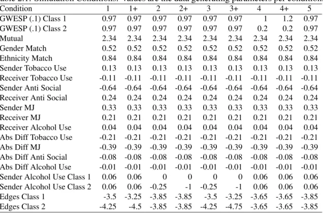
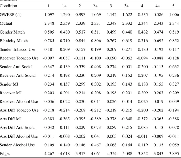
There were 9 simulation conditions in total (See Table 2.1). Simulation conditions
were arrived at by examining the parameter estimates from the empirical model and
chang-ing some of the parameter values to reflect different situations. For example, the empirical
For condition 1 of the simulations, which only modeled a heterogeneous effect of the edge
term, the parameter for sender alcohol use was set to be equal across both classes.
Addi-tionally, for all conditions the edge parameter was increased from the empirical example to
simulate less sparse matrices and therefore increase the amount of information in the data.
Finally, in all conditions, approximately 25% of nodes were in class 2. This was derived
from the empirical results.
Four out of the 9 simulation conditions were replications of conditions, but with
in-creased effect sizes. These inin-creased effect size conditions are denoted with a +. Inin-creased
effect sizes were assessed to get a sense of what approximate effect sizes return accurate
latent class labeling. Condition 1 and Condition 1+ simulated networks with two latent
classes that differed only in the edge parameter. Condition 2 and Condition 2+ simulated
networks with two latent classes that differed only in the effect of a sender nodal attribute
(alcohol use) . Condition 3 and Condition 3+ simulated networks with two latent classes
that differed only in the effect of sender nodal attribute and the edge parameter.
Condi-tion 4 and CondiCondi-tion 4+ simulated networks with two latent classes that differed only in
the GWESP effect. Note that the homogeneous edge effect for Conditions 4 and 4+ was
increased from -3.85 to -3.65 to ensure that the total edge count in Condition 4 and 4+ was
comparable to the edge count in other conditions. Finally, Condition 5 generated networks
with no latent class structure. Simulation parameters are presented in Table 2.1.
In Conditions 1 through 4 and 1a though 4a, correctly specified models were fit to
the data as well as homogeneous models. In Condition 5 a model that specified 2 latent
classes and heterogeneity on the sender alcohol use parameter and the edges parameter was
estimated, along with a homogeneous model.
Raw and relative bias were assessed, as well as computed standard errors from the
sim-ulation set and average estimated standard errors. Additionally, Rand Indices and Adjusted
Table 2.1: Simulation Conditions: Values are the data generating parameters per condition.
Condition 1 1+ 2 2+ 3 3+ 4 4+ 5
GWESP (.1) Class 1 0.97 0.97 0.97 0.97 0.97 0.97 1 1.2 0.97 GWESP (.1) Class 2 0.97 0.97 0.97 0.97 0.97 0.97 0.2 0.2 0.97 Mutual 2.34 2.34 2.34 2.34 2.34 2.34 2.34 2.34 2.34 Gender Match 0.52 0.52 0.52 0.52 0.52 0.52 0.52 0.52 0.52 Ethnicity Match 0.84 0.84 0.84 0.84 0.84 0.84 0.84 0.84 0.84 Sender Tobacco Use 0.13 0.13 0.13 0.13 0.13 0.13 0.13 0.13 0.13 Receiver Tobacco Use -0.11 -0.11 -0.11 -0.11 -0.11 -0.11 -0.11 -0.11 -0.11 Sender Anti Social -0.64 -0.64 -0.64 -0.64 -0.64 -0.64 -0.64 -0.64 -0.64 Receiver Anti Social 0.24 0.24 0.24 0.24 0.24 0.24 0.24 0.24 0.24 Sender MJ 0.33 0.33 0.33 0.33 0.33 0.33 0.33 0.33 0.33 Receiver MJ 0.21 0.21 0.21 0.21 0.21 0.21 0.21 0.21 0.21 Receiver Alcohol Use 0.04 0.04 0.04 0.04 0.04 0.04 0.04 0.04 0.04 Abs Diff Tobacco Use -0.21 -0.21 -0.21 -0.21 -0.21 -0.21 -0.21 -0.21 -0.21 Abs Diff MJ -0.39 -0.39 -0.39 -0.39 -0.39 -0.39 -0.39 -0.39 -0.39 Abs Diff Anti Social -0.08 -0.08 -0.08 -0.08 -0.08 -0.08 -0.08 -0.08 -0.08 Abs Diff Alcohol Use -0.01 -0.01 -0.01 -0.01 -0.01 -0.01 -0.01 -0.01 -0.01 Sender Alcohol Use Class 1 0.06 0.06 0 0 0 0 0.06 0.06 0.06 Sender Alcohol Use Class 2 0.06 0.06 -0.25 -1 -0.25 -1 0.06 0.06 0.06 Edges Class 1 -3.5 -3.25 -3.85 -3.85 -3.5 -3.25 -3.65 -3.65 -3.85 Edges Class 2 -4.25 -4.5 -3.85 -3.85 -4.25 -4.75 -3.65 -3.65 -3.85
MJ: Marijuana, Abs Diff: Absolute Difference
class labels and the true latent class labels. This indicates performance of the method, in
that if the method failed to detect true latent class labels for a condition, the method would
have not performed well with that parameter set. Both Rand Index and Adjusted Rand
In-dex are presented. Rand InIn-dex is a raw measure of agreement between two sets of labels,
while the Adjusted Rand Index is a measure of agreement that accounts for the expected
level of agreement if the labels were assigned randomly. Finally, Rand and Adjusted Rand
are presented for the latent class labels of only the nodes that had a value higher than 0
for alcohol use. These results are presented as there are several conditions where the latent
classes are in part defined on the effect of sender alcohol use. If alcohol use is 0 for an
individual, and the latent classes are defined wholly on alcohol use, then the node with no
alcohol use would be assigned to any latent class at random. By examining the subset of
All conditions had 500 networks simulated. The networks were simulated using the
MCMC approach used in the R package statnet (Handcock, Hunter, Butts, Goodreau &
Morris, 2003). This approach randomly toggles edges within a network with the
probabil-ity according to the generating model. This allows the simulated data to properly reflect
transitivity, as well as contain sampling variability. To clarify, only the networks
them-selves were simulated. The covariate data set was the same across all simulations as was
the true latent class labeling.
Estimation of these models used twenty random start values per trial as per the
algo-rithm described above.
2.2 Simulation Results for Heterogeneous Models
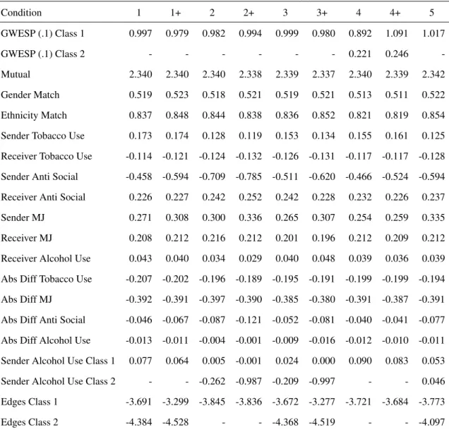
Table 2.2 contains the estimated parameters for the heterogeneous models, while Table
2.3 shows the mean Rand Indices and Adjusted Rand Indices for latent class recovery for
every individual, as well as individuals who use alcohol. Table 2.4 contains the relative bias
and Table 2.5 contains the raw bias. Table 2.6 presents average estimated standard error
and standard deviation of the estimates across the simulated networks. Finally, Table 2.7
contains the mean probability of class membership, and standard deviation of class
mem-bership for correctly and incorrectly classified nodes across all conditions. As described
below, these simulations indicate that the model can recover true latent class structure, and
Table 2.2: Mean Estimated Parameters calculated across 500 trials in each condition
Condition 1 1+ 2 2+ 3 3+ 4 4+ 5
GWESP (.1) Class 1 0.997 0.979 0.982 0.994 0.999 0.980 0.892 1.091 1.017
GWESP (.1) Class 2 - - - 0.221 0.246
-Mutual 2.340 2.340 2.340 2.338 2.339 2.337 2.340 2.339 2.342
Gender Match 0.519 0.523 0.518 0.521 0.519 0.521 0.513 0.511 0.522
Ethnicity Match 0.837 0.848 0.844 0.838 0.836 0.852 0.821 0.819 0.854
Sender Tobacco Use 0.173 0.174 0.128 0.119 0.153 0.134 0.155 0.161 0.125
Receiver Tobacco Use -0.114 -0.121 -0.124 -0.132 -0.126 -0.131 -0.117 -0.117 -0.128
Sender Anti Social -0.458 -0.594 -0.709 -0.785 -0.511 -0.620 -0.466 -0.524 -0.594
Receiver Anti Social 0.226 0.227 0.242 0.252 0.242 0.228 0.232 0.226 0.237
Sender MJ 0.271 0.308 0.300 0.336 0.265 0.307 0.254 0.259 0.335
Receiver MJ 0.208 0.212 0.216 0.212 0.201 0.196 0.212 0.209 0.212
Receiver Alcohol Use 0.043 0.040 0.034 0.029 0.040 0.048 0.039 0.036 0.039
Abs Diff Tobacco Use -0.207 -0.202 -0.196 -0.189 -0.195 -0.191 -0.199 -0.199 -0.194
Abs Diff MJ -0.392 -0.391 -0.397 -0.390 -0.385 -0.380 -0.391 -0.387 -0.391
Abs Diff Anti Social -0.046 -0.067 -0.087 -0.121 -0.052 -0.081 -0.040 -0.041 -0.077
Abs Diff Alcohol Use -0.013 -0.011 -0.004 -0.001 -0.009 -0.016 -0.012 -0.010 -0.011
Sender Alcohol Use Class 1 0.077 0.064 0.005 -0.001 0.024 0.000 0.090 0.083 0.053
Sender Alcohol Use Class 2 - - -0.262 -0.987 -0.209 -0.997 - - 0.046
Edges Class 1 -3.691 -3.299 -3.845 -3.836 -3.672 -3.277 -3.721 -3.684 -3.773
Edges Class 2 -4.384 -4.528 - - -4.368 -4.519 - - -4.097
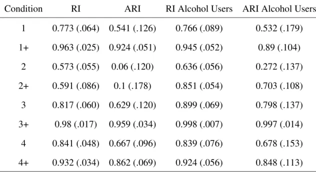
Table 2.3: Mean Rand Indices and Adjusted Rand Indices (Standard Deviations computed
from the sample) computed across 500 trials within each condition. Results indicate best
recovery occurs in the + conditions, with higher class separation. Structural effects such as
GWESP are also recovered well.
Condition
RI
ARI
RI Alcohol Users
ARI Alcohol Users
1
0.773 (.064)
0.541 (.126)
0.766 (.089)
0.532 (.179)
1+
0.963 (.025)
0.924 (.051)
0.945 (.052)
0.89 (.104)
2
0.573 (.055)
0.06 (.120)
0.636 (.056)
0.272 (.137)
2+
0.591 (.086)
0.1 (.178)
0.851 (.054)
0.703 (.108)
3
0.817 (.060)
0.629 (.120)
0.899 (.069)
0.798 (.137)
3+
0.98 (.017)
0.959 (.034)
0.998 (.007)
0.997 (.014)
4
0.841 (.048)
0.667 (.096)
0.839 (.076)
0.678 (.153)
4+
0.932 (.034)
0.862 (.069)
0.924 (.056)
0.848 (.113)
Rand Indices and Adjusted Rand Indices were computed as the empirical mean and
empirical standard deviation over every trial in a given condition. These are not analytic
results from a hyper-geometric distribution and are not meant to test for significance. For
class recovery, the mean adjusted Rand indices contained in Table 2.3 indicate that across
all simulation conditions, increasing the difference between the latent classes leads to
in-creased recovery of the latent classes. However, for conditions with smaller class separation
(Conditions 1, 2, 3, 4), the recovery of the latent classes was not optimal. This is likely due
to the use of the classification likelihood, which doesn’t perform well for classes that are
ill-separated. For most conditions, the greatest improvement in recovery of the latent class
labels occurred only when looking at alcohol users. Conditions 2 and 2+ reveals even at
larger differences between the latent classes, recovery of the class labels for alcohol users
respectively). This is likely due to the latent class being defined solely on individuals who
used alcohol, a subset of the sample, as opposed to other conditions that had the latent
classes also be defined by structural parameters such as edges or GWESP.
These results indicates caution when using a latent class ERGM, as the effect size for a
latent class that is wholly defined by a covariate needs to be larger than the effect size for a
latent class that is defined by covariates and network structures. Additionally, with the use
of classification likelihood, caution should be taken when analyzing a network to ensure
that theoretically the classes are well separated.
One set of results of note is that Condition 4 and 4+ had remarkably good recovery
of the latent class labels, even at at the lower class difference (ARI of .667 and .862 for
Condition 4 and 4+ respectively). This suggests that heterogeneities in the GWESP term
are reflected strongly in observed network structure. Finally, standard deviations of the
Adjusted Rand Indices suggest that there was variability in recovery rates due to sampling
fluctuations. This variability can lead, particularly in conditions with low class
separa-tion, to very poor rates of classification. As one would expect, there is more variability
in the ARIs the lower the average ARI becomes, again, suggesting that the classification
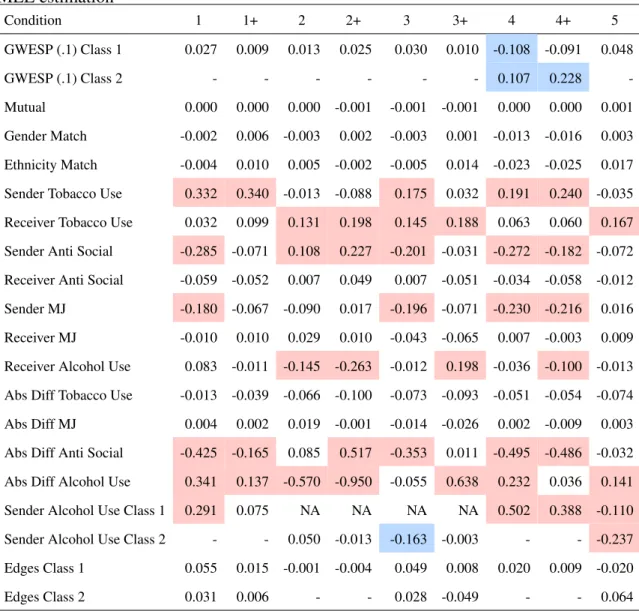
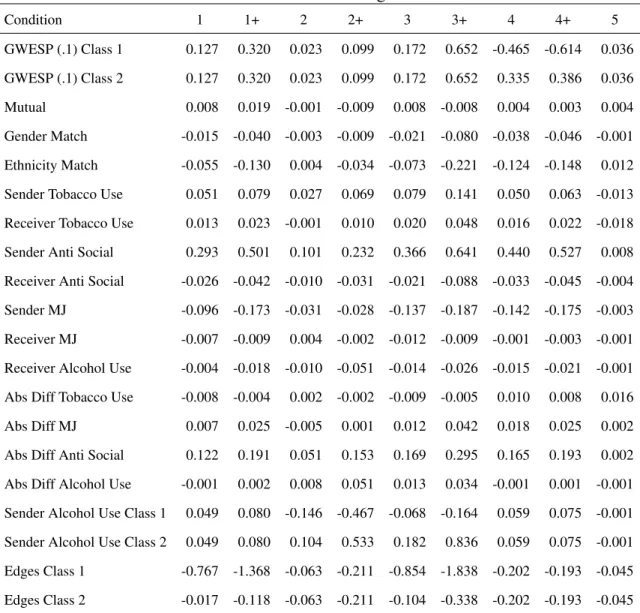
Table 2.4: Relative Bias in the Parameter Estimates For Heterogeneous Models, calculated
using Mean Raw Bias over True Parameter Value. Results indicate modest levels of bias
in homogeneous parameters. This bias is in line with expected bias from the approximate
MLE estimation
Condition 1 1+ 2 2+ 3 3+ 4 4+ 5
GWESP (.1) Class 1 0.027 0.009 0.013 0.025 0.030 0.010 -0.108 -0.091 0.048
GWESP (.1) Class 2 - - - 0.107 0.228
-Mutual 0.000 0.000 0.000 -0.001 -0.001 -0.001 0.000 0.000 0.001
Gender Match -0.002 0.006 -0.003 0.002 -0.003 0.001 -0.013 -0.016 0.003
Ethnicity Match -0.004 0.010 0.005 -0.002 -0.005 0.014 -0.023 -0.025 0.017
Sender Tobacco Use 0.332 0.340 -0.013 -0.088 0.175 0.032 0.191 0.240 -0.035
Receiver Tobacco Use 0.032 0.099 0.131 0.198 0.145 0.188 0.063 0.060 0.167
Sender Anti Social -0.285 -0.071 0.108 0.227 -0.201 -0.031 -0.272 -0.182 -0.072
Receiver Anti Social -0.059 -0.052 0.007 0.049 0.007 -0.051 -0.034 -0.058 -0.012
Sender MJ -0.180 -0.067 -0.090 0.017 -0.196 -0.071 -0.230 -0.216 0.016
Receiver MJ -0.010 0.010 0.029 0.010 -0.043 -0.065 0.007 -0.003 0.009
Receiver Alcohol Use 0.083 -0.011 -0.145 -0.263 -0.012 0.198 -0.036 -0.100 -0.013
Abs Diff Tobacco Use -0.013 -0.039 -0.066 -0.100 -0.073 -0.093 -0.051 -0.054 -0.074
Abs Diff MJ 0.004 0.002 0.019 -0.001 -0.014 -0.026 0.002 -0.009 0.003
Abs Diff Anti Social -0.425 -0.165 0.085 0.517 -0.353 0.011 -0.495 -0.486 -0.032
Abs Diff Alcohol Use 0.341 0.137 -0.570 -0.950 -0.055 0.638 0.232 0.036 0.141
Sender Alcohol Use Class 1 0.291 0.075 NA NA NA NA 0.502 0.388 -0.110
Sender Alcohol Use Class 2 - - 0.050 -0.013 -0.163 -0.003 - - -0.237
Edges Class 1 0.055 0.015 -0.001 -0.004 0.049 0.008 0.020 0.009 -0.020
Edges Class 2 0.031 0.006 - - 0.028 -0.049 - - 0.064
MJ: Marijuana, Abs Diff: Absolute Difference, NAs due to true effect being 0.
Red highlights indicates relative bias in homogeneous parameters above .1, blue
high-lights indicate relative bias in heterogeneous parameters above .1.
term (GWESP Class 2), which had a true value of .2 in both conditions, was the worst.
The relative bias here was .107 for Condition 4 and .228 for Condition 4+. However, the
raw bias (contained below in Table 2.5) in terms of magnitude was quite small, .021 and
.046 respectively. This level of bias is not relevant to researchers analyzing empirical data,
and is likely due to the GWESP term being difficult to estimate in general. The one other
heterogeneous term that had a relative bias of above .1 was that of Sender Alcohol Use in
Class 2 for Condition 3. The relative bias for this parameter was -.163, with a raw bias of
.041. The true parameter value was -.25, which suggests that while the relative bias was
high, the actual level of raw bias was comparatively low.
The homogeneous parameters recovery (such as gender match, ethnicity match, etc.)
was reasonable with very few parameters having greater than .1 absolute raw bias or greater
than .1 relative bias. However the Sender Anti Social effect for conditions 1, 2+, 3, 4,
and 4+ all have raw bias magnitude greater than .1. This effect was held homogeneous
across all conditions and had the highest magnitude of the homogeneous effects (-.64). The
patterning of bias across all conditions was not consistent, and this likely indicates that
the effect was being disrupted by the effects of the structural parameters such as GWESP.
Additionally, with Sender Tobacco Use, several conditions had relative bias greater than .1.
However, the true effect of Sender Tobacco Use was small (.13) in all conditions, which
can lead to small levels of raw bias translating into large relative bias.
This occurrence of high relative biases for very small true parameters is expected and
most notably occurs for the Absolute Difference of Anti-Social Behavior, Sender Alcohol
use (for models with homogeneous Sender Alcohol Use), and Absolute Difference in
Al-cohol Use. Furthermore, for conditions 2, 2+, 3 and 3+ the true effect of Sender AlAl-cohol
Use in Class 1 was 0, which would lead to undefined relative bias for any level of raw bias.
As for Condition 5, recovery of homogeneous parameters was quite good, with no raw
the mis-specification of the latent class structure did not lead to systematic bias in the
homogeneous parameters. Additionally, the spread of the latent class parameters around
the true homogeneous parameters was quite reasonable, with Sender Alcohol Use having a
true effect of .06, and the latent classes returning an effect of .053 and .046, while the Edge
effect is 3.85 while the latent classes returned effects of 3.773 and 4.097 respectively.
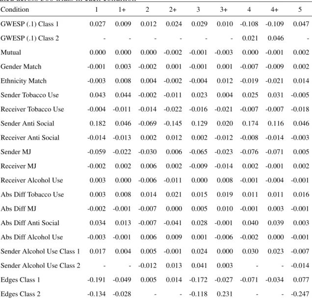
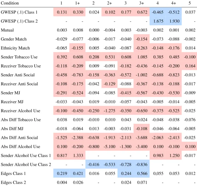
Table 2.5: Mean Raw Bias in the Parameter Estimates for Heterogeneous Models,
calcu-lated across 500 trials in each condition
Condition 1 1+ 2 2+ 3 3+ 4 4+ 5
GWESP (.1) Class 1 0.027 0.009 0.012 0.024 0.029 0.010 -0.108 -0.109 0.047
GWESP (.1) Class 2 - - - 0.021 0.046
-Mutual 0.000 0.000 0.000 -0.002 -0.001 -0.003 0.000 -0.001 0.002
Gender Match -0.001 0.003 -0.002 0.001 -0.001 0.001 -0.007 -0.009 0.002
Ethnicity Match -0.003 0.008 0.004 -0.002 -0.004 0.012 -0.019 -0.021 0.014
Sender Tobacco Use 0.043 0.044 -0.002 -0.011 0.023 0.004 0.025 0.031 -0.005
Receiver Tobacco Use -0.004 -0.011 -0.014 -0.022 -0.016 -0.021 -0.007 -0.007 -0.018
Sender Anti Social 0.182 0.046 -0.069 -0.145 0.129 0.020 0.174 0.116 0.046
Receiver Anti Social -0.014 -0.013 0.002 0.012 0.002 -0.012 -0.008 -0.014 -0.003
Sender MJ -0.059 -0.022 -0.030 0.006 -0.065 -0.023 -0.076 -0.071 0.005
Receiver MJ -0.002 0.002 0.006 0.002 -0.009 -0.014 0.002 -0.001 0.002
Receiver Alcohol Use 0.003 0.000 -0.006 -0.011 0.000 0.008 -0.001 -0.004 -0.001
Abs Diff Tobacco Use 0.003 0.008 0.014 0.021 0.015 0.019 0.011 0.011 0.016
Abs Diff MJ -0.002 -0.001 -0.007 0.000 0.005 0.010 -0.001 0.003 -0.001
Abs Diff Anti Social 0.034 0.013 -0.007 -0.041 0.028 -0.001 0.040 0.039 0.003
Abs Diff Alcohol Use -0.003 -0.001 0.006 0.009 0.001 -0.006 -0.002 0.000 -0.001
Sender Alcohol Use Class 1 0.017 0.004 0.005 -0.001 0.024 0.000 0.030 0.023 -0.007
Sender Alcohol Use Class 2 - - -0.012 0.013 0.041 0.003 - - -0.014
Edges Class 1 -0.191 -0.049 0.005 0.014 -0.172 -0.027 -0.071 -0.034 0.077
Edges Class 2 -0.134 -0.028 - - -0.118 0.231 - - -0.247
In summary, Tables 2.4 and 2.5 suggest that the sender latent class models fit to
hetero-geneous data do a reasonable job at recovering the model parameters. Bias in the parameter
estimates is in part due to ERG modeling being approximate even when using the
MCMC-MLE. A degree of bias is to be expected. That being said, the fact that bias still remained
even when fitting the generating model to data suggests that researchers should have
strin-gent criteria for interpreting results from latent class ERGMs, interpreting both effect size
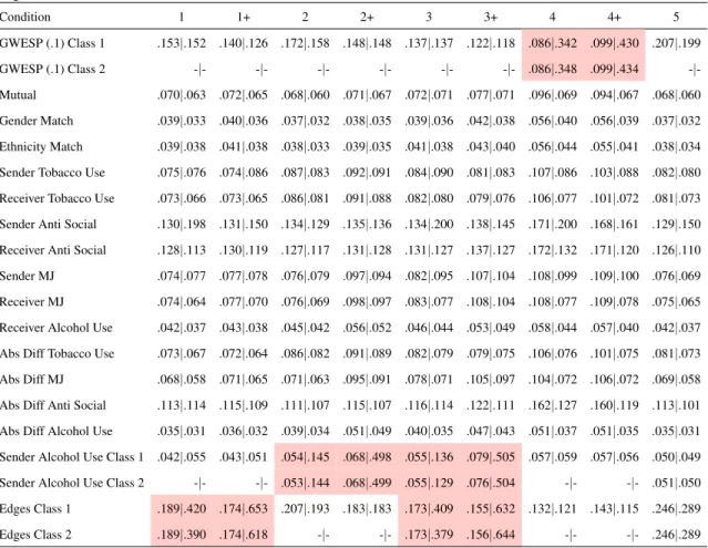
Table 2.6: Mean Estimated Standard Error calculated across 500 trials per condition|
Sim-ulation Error calculated from the difference between the parameter estimates and the true
parameter estimates across 500 trials per condition - Heterogeneous Networks. Results
indicate disagreement between estimated standard error and simulation error due to the
implementation of classification likelihood estimation.
Condition 1 1+ 2 2+ 3 3+ 4 4+ 5
GWESP (.1) Class 1 .153|.152 .140|.126 .172|.158 .148|.148 .137|.137 .122|.118 .086|.342 .099|.430 .207|.199
GWESP (.1) Class 2 -|- -|- -|- -|- -|- -|- .086|.348 .099|.434 -|
-Mutual .070|.063 .072|.065 .068|.060 .071|.067 .072|.071 .077|.071 .096|.069 .094|.067 .068|.060
Gender Match .039|.033 .040|.036 .037|.032 .038|.035 .039|.036 .042|.038 .056|.040 .056|.039 .037|.032
Ethnicity Match .039|.038 .041|.038 .038|.033 .039|.035 .041|.038 .043|.040 .056|.044 .055|.041 .038|.034
Sender Tobacco Use .075|.076 .074|.086 .087|.083 .092|.091 .084|.090 .081|.083 .107|.086 .103|.088 .082|.080
Receiver Tobacco Use .073|.066 .073|.065 .086|.081 .091|.088 .082|.080 .079|.076 .106|.077 .101|.072 .081|.073
Sender Anti Social .130|.198 .131|.150 .134|.129 .135|.136 .134|.200 .138|.145 .171|.200 .168|.161 .129|.150
Receiver Anti Social .128|.113 .130|.119 .127|.117 .131|.128 .131|.127 .137|.127 .172|.132 .171|.120 .126|.110
Sender MJ .074|.077 .077|.078 .076|.079 .097|.094 .082|.095 .107|.104 .108|.099 .109|.100 .076|.069
Receiver MJ .074|.064 .077|.070 .076|.069 .098|.097 .083|.077 .108|.104 .108|.077 .109|.078 .075|.065
Receiver Alcohol Use .042|.037 .043|.038 .045|.042 .056|.052 .046|.044 .053|.049 .058|.044 .057|.040 .042|.037
Abs Diff Tobacco Use .073|.067 .072|.064 .086|.082 .091|.089 .082|.079 .079|.075 .106|.076 .101|.075 .081|.073
Abs Diff MJ .068|.058 .071|.065 .071|.063 .095|.091 .078|.071 .105|.097 .104|.072 .106|.072 .069|.058
Abs Diff Anti Social .113|.114 .115|.109 .111|.107 .115|.107 .116|.114 .122|.111 .162|.127 .160|.119 .113|.101
Abs Diff Alcohol Use .035|.031 .036|.032 .039|.034 .051|.049 .040|.035 .047|.043 .051|.037 .051|.035 .035|.031
Sender Alcohol Use Class 1 .042|.055 .043|.051 .054|.145 .068|.498 .055|.136 .079|.505 .057|.059 .057|.056 .050|.049
Sender Alcohol Use Class 2 -|- -|- .053|.144 .068|.499 .055|.129 .076|.504 -|- -|- .051|.050
Edges Class 1 .189|.420 .174|.653 .207|.193 .183|.183 .173|.409 .155|.632 .132|.121 .143|.115 .246|.289
Edges Class 2 .189|.390 .174|.618 -|- -|- .173|.379 .156|.644 -|- -|- .246|.289
MJ: Marijuana, Abs Diff: Absolute Difference
Red Highlights indicate substantial disagreement between mean estimated standard
er-ror and simulation erer-ror.
As for estimated standard errors of the estimates and the standard deviations across
the simulation trials for every homogeneous parameter the estimated standard error and
the standard deviation of the parameter across the condition agreed. However, for the
simulation standard deviation (Table 2.6 highlighted to show). This is in part due to error in
classification across the simulation trials. If there are simulation trials where the individuals
are mis-classified then the estimates of the heterogeneous effects will be more variable than
if in every trial the latent class labels were recovered with perfect fidelity. Additionally, the
estimated standard errors assume that the latent class assignment is the true assignment, and
are not adjusted for uncertainty in class assignment. This is a reflection of the hard-type
EM algorithm in use in the estimation.
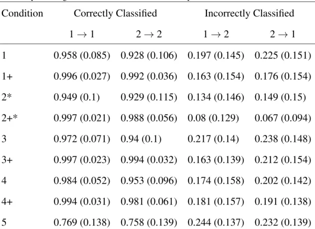
Table 2.7: Mean Posterior Class Probabilities For True Class Assignment for both correctly
classified and incorrectly classified nodes (Standard Deviation), calculated over 500 trials
for each condition. Results indicate that when nodes are correctly classified, they have a
high probability of being in the correct class. When nodes are incorrectly classified, the
probability of being in the correct class is substantially lower than .5.