The Effect of Dealing in Securities on Lending
at Commercial Banks
Dinara Bayazitova
A dissertation submitted to the faculty of the University of North Carolina at Chapel Hill in partial fulfillment of the requirements for the degree of Doctor of Philosophy in
the Department of Finance, Kenan Flagler Business School.
Chapel Hill
2013
Approved by:
Greg Brown
Robert Bushman
Paolo Fulghieri
Matthias Kahl
ABSTRACT
DINARA BAYAZITOVA: The Effect of Dealing in Securities on Lending at Commercial Banks
(Under the direction of Anil Shivdasani)
This study empirically examines the effect on lending of the change in bank regulation in
1996, when commercial banks were allowed to increase their dealing in securities. It
documents the decline in loan growth rates at the affected dealer banks compared to
unaffected banks. In particular, affected banks restricted their supply of lending by
increasing denial rates on mortgages after the change. These effects can be explained by
the competition for limited funding between lending and dealing in securities in the
presence of credit constraints. Also, this research demonstrates that dealer banks shift
funds from lending to market-making during periods of high volatility. This occurs
because of the increased demand for liquidity provision by market-makers. Consistent
with this explanation, I find higher risk-adjusted gross trading returns at dealer banks at
ACKNOWLEDGEMENTS
For their helpful comments and suggestions, I would like to thank Greg Brown, Anil
Shivdasani, Matthias Kahl, Paolo Fulghieri, Jennifer Conrad, Diego Garcia, Pab
Jotikasthira, Paige Ouimet, Ed Van Wesep, David Ravenscraft, Robert Bushman, and
seminar participants at the University of North Carolina. people. I am especially grateful
TABLE OF CONTENTS.
LIST OF TABLES………...………viii
1. Introduction……….………..…..…5
2. Data………..………..……10
3. Exogenous Shock I: Regulatory Change in 1996………..……12
3.1. Bank regulation of dealing in securities in the US……….13
3.2. Hypothesis I: Competition between lending and dealing for funding……....16
3.3. Exogenous shock I: The regulatory change of 1996………...17
3.4. Results: Changes in loan growth after the regulatory change of 1996……...18
3.5. Results: Aggregate lending implications of the regulatory change of 1996………...….19
3.6. What drives reduction in loan growth: demand or supply?...20
3.7. Which type of borrowers experience a reduction in credit availability?...23
3.8. Alternative explanations……….24
4. Exogenous Shock II: Intensified Capital Market Frictions during Periods of High Uncertainty 4.1. Incentives in market making during periods of high uncertainty…………...25
4.2. Trading returns and trading assets of dealer banks during high uncertainty periods………….………..………...…...28
4.3. Lending by dealer banks during high uncertainty periods…………..………30
4.4 Alternative explanations……….……….31
LIST OF TABLES
1. Summary statistics for dealer banks………...33
2. Loan growth at dealer banks after the regulatory change I:
difference-in-difference tests………..………..……….……34
3. Decline in loan growth at dealer banks after the regulatory change II:
regression analysis……….……....35
4. Mortgage application denial rates at dealer banks after the regulatory
change………....…36
5. Securitization rates at dealer banks after the regulatory
change………...……….………...………...……..38
6. Trading returns and trading assets of dealer banks at high uncertainty
periods……...………...………...…39
7. Lending by dealer banks at high uncertainty periods:
Difference-in-difference tests………..……….……….40
8. Lending by dealer banks at high uncertainty periods: multivariate analysis...…..41
9. Lending by dealer banks: recessions and funding type……….42
1.Introduction
In this thesis I consider patterns of lending behavior by conglomerate banks that combine
lending with dealing in securities. I analyze how lending by this kind of banks is different from
lending by other commercial banks. Proprietary trading and dealing in securities by commercial
banks is a controversial topic. One of the major points of the debate is how to distinguish
between these two types of trading. Many academics and industry practitioners agree that there is
no clear algorithm to implement such a distinction. Even more importantly, it may be
conceptually impossible, since market making can be viewed as a form of proprietary trading
(Duffie, 2012). If this is taken into account, one can expect that proposed restrictions on
proprietary trading will limit market making. They might also have unintended consequences in
the form of reduced liquidity and increased funding costs for bond issuers (Oliver Wyman,
2011).
In addition to its effect on bank risk and liquidity in financial markets, there is another
dimension to the possible consequences of trading in securities by commercial banks: it may
affect bank lending. And it is this effect that is the main focus of this empirical study. It is not
well understood, despite recent attention to commercial banks that engage in both lending and
trading. It is very important, however, for formulating a sound regulatory policy, given that
dealer banks account for a large portion of total lending in the US.
Trading in securities by commercial banks may have a negative effect on their lending.
allocated to both issued loans and trading assets held on balance sheets. When trading and
lending divisions are combined in one financial institution, they compete for a limited amount of
bank equity capital. Capital is costly, however, and if the expected risk-adjusted performance of
lending is lower than that of trading, it may get less capital. Because trading at commercial banks
is restricted and minimum capital requirements limit the opportunities for a bank to take risk, it
will choose an optimal mix of lending and trading. If expected returns are non-linear, however,
an internal rather than the corner solution will be chosen.
As a way of resolving the issue of causality, I consider two exogenous shocks to dealing
and examine their effects on lending at the affected banks. First, I look at the bank regulatory
change of 1996 that relaxed the constraint on dealing by commercial banks. For a long time the
Banking Act of 1933 (also known as the Glass-Steagall Act) prohibited commercial banks, with
a few exceptions, from making markets in securities. This restriction was subsequently eroded by
the Federal Reserve’s reinterpretations of its wording. In 1987 commercial banks were allowed
to establish so called Section 20 subsidiaries that could engage in underwriting and dealing in
securities to a limited extent. In 1996 this constraint was further relaxed. It is this later change in
the rule that is used as an exogenous shock to examine the effect of dealing on lending in this
thesis. To eliminate the contaminating influence of other events affecting both types of banks, I
perform a difference-in-difference test. I find that after the constraint on dealing was relaxed,
dealer banks reduced their loan growth compared to other banks not affected by the regulatory
change.
It is also important to understand what drives the decline in loan growth by dealer banks
after the regulatory change: lower loan supply or decline in loan demand. To disentangle loan
compare the changes in this likelihood after 1996 between dealer and other banks. To perform
this test I consider mortgage loans only, because this is the only category for which such detailed
data is publicly available. I find that after 1996 dealer banks were more likely to reject mortgage
applications than were other banks. In other words, dealer banks tightened their mortgage loan
supply after the constraint on market making was relaxed. This result holds when I repeat the
analysis for each of the ten largest US states separately to form a better match between affected
and unaffected banks. Finally, to provide evidence in support of the supply-side explanation, I
examine changes in loan demand around the bank regulatory change. I measure loan demand by
the total number of mortgage applications submitted to a bank, and show that changes in
mortgage demand was no different for dealer banks compared to others.
I also examine alternative explanations for the decline in loan growth rate for dealer
banks after the regulatory change. One can argue that loan demand has declined because
commercial banks entered underwriting at the same time as dealing in securities. Although this
could magnify the magnitude of the decline in corporate loans, it was unlikely to affect
mortgages, for which I find tightening of credit supply as well.
Another concern is that banks do not hold on their balance sheets only loans they have
originated, but also securitized. Therefore, the decline in growth rates for loans held on bank
balance sheets might be due to an overall upward trend in securitization, which is likely to affect
larger banks more than smaller ones. However, we do not find support for this explanation, since
there is no difference in changes in the fraction of securitized mortgages held by dealer and
Increase in demand for dealing on capital markets during high-volatility periods is
considered the second exogenous shock. Asset pricing literature suggests that at periods of high
uncertainty, demand for dealing is particularly strong. There are both theoretical reasons and
empirical evidence of this effect. So called flight to quality usually arises at these times, and
requires market-makers to provide liquidity. Also, investors tend to increase their hedging
demands at those times as well. Selling pressure is further amplified by a number of frictions
discussed in the asset pricing literature. In particular, fund managers are subject to withdrawals
when fund performance falls below a threshold (Vayanos, 2004). Traders liquidate holdings
across different securities after trading losses (Kyle & Xiong, 2001). There is a positive relation
between volatility and trading volume for different types of assets (Gallant, Rossi & Tauchen,
1992; Foster, 1995; Wang and Yau, 2000; Fleming 2003). As a result of these frictions, at
periods of high uncertainty financial institutions that combine lending and dealing under one
umbrella are likely to have incentives to move funds from lending to dealing.
The empirical evidence that I provide is consistent with this hypothesis. High-volatility
periods are defined as the quarters when the average daily VIX was in the top 25% of quarters
since the beginning of the VIX series in 1990. I find that during these periods banks have
abnormally high risk-adjusted gross trading returns, suggesting that they do have incentives to
move funds from lending to dealing. I also show that during periods of high volatility, growth
rates in trading assets increase while loan growth rates decrease for these banks relative to others.
This suggests that dealer banks do shift funds from lending to dealing at these times.
I consider and reject some alternative explanations for these findings. First, I show that
the lower growth rate in loans by dealer banks during high-volatility periods is not due to the
recessions. Second, I show that the result cannot be explained by high reliance of these banks on
financing from capital markets, which tend to dry up during periods of high volatility.
The findings of this thesis have important implications for bank regulation. Most
importantly, combining lending and market-making may divert funds from lending and is likely
to lower loan growth. At periods of high volatility this effect is likely to be amplified.
However, it is also possible that higher profits from market-making may compensate for
abnormally high credit losses, thus supporting bank capital when recessions are accompanied by
high volatility on capital markets. Banks with higher levels of capital are likely to lend more.
Therefore, profits from market-making may indirectly increase lending in later periods. In other
words, market-making can potentially subsidize lending through diversification of bank earnings.
Although these indirect positive effects of trading on lending are possible, they are difficult to
measure, and I do not provide supporting evidence in this thesis.
This thesis contributes to the literature on trading in securities by commercial banks. The
majority of the earlier papers have focused on the effect of trading in securities on bank risk.
Their findings are mixed because of the different methodologies and sample periods used.
Studies from the 1980s find that overall commercial bank risk is lower in the presence of trading.
This is an example of a classic diversification effect that arises when two types of activities are
combined, and conditional on their earnings being less than perfectly correlated. Wall and
Eisenbeis (1984) consider combined earnings of banks and securities firms at the industry level.
White (1986) finds that banks trading in securities had higher survival rates than others during
the Great Depression. Kwast (1989) finds some potential for diversification gains from limited
appears to be limited. Later studies find an increase in overall bank risk after the Glass-Steagall
Act was repealed (Geyfman & Yeager, 2009) and for Section 20 subsidiaries using their
confidential financial statements (Kwan, 1998). DeYoung and Roland (2001) analyze the reasons
for higher volatility of earnings from trading than from lending. They suggest that in contrast to
lending, trading has low switching costs (relationships are not as important as they are in
lending) and high operating leverage (the competitive salaries of traders are a large fixed
expense). None of these papers, however, considered the effect of trading on lending, the focus
of this study.
The findings of this thesis are relevant for the current discussion of the so-called Volcker
rule, one of the most intensely debated parts of the Dodd-Frank Wall Street Reform and
Consumer Protection Act (Johnson, 2012). The Volcker rule constrains trading by commercial
banks and is intended to limit risk-taking in the banking sector that is financed to a large extent
through FDIC insured deposits. The Volcker rule limits proprietary trading and investments in
hedge funds by commercial banks to 3% of bank capital, but allows them to trade “on behalf of
customers” (to make markets). Although this rule applies only to proprietary trading and does
not restrict dealing in securities, it is reasonable to argue that it might affect lending as well,
because the two types of trading are difficult to distinguish.
This thesis is organized as follows. In Section 2, the data and sample construction are
described. In Section 3 the effect of regulatory change on lending by dealer banks is considered.
In Section 4 the incentives in lending and market-making during periods of high volatility are
considered. In Section 5 the findings are summarized.
Banks dealers are bank holding companies (BHCs) that have established so-called Section 20
subsidiaries. The list of these banks is compiled on the basis of the approval decisions for
establishing Section 20 subsidiaries obtained from the Federal Reserve Bulletins. As of the end
of the second quarter of 1995, 25 BHCs in US had established Section 20 subsidiaries. These
banks are listed in Appendix A. The subsample of nondealers consists of 1,082 bank holding
companies, including 398 public banks.
Bank financial statements data are obtained from Y-9C Reports (the Bank Holding Company
Report of Income and Report of Condition) for the years from 1995 until 2008. Table 1 shows
summary statistics on the major characteristics of dealer banks that are used as control variables
in regressions later. Chargeoffs on loans as a percentage of total loans on bank balance sheet are
used as a proxy for credit losses. The percentage of total assets financed with deposits shows the
composition of funding.
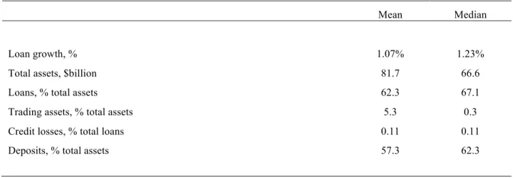
Loan balances at dealer banks grew on average 1.07% per quarter in 1995–2008. The median
growth rate was slightly higher at 1.23%. As of the end of the second quarter of 1995, banks with
Section 20 subsidiaries had on average $81.7 billion in total assets. They had 62.3% of their
assets invested in loans and 5.3% in trading assets. Credit losses were on average 0.11% of total
loans. 57.3% of total assets were funded with deposits.
Data on mortgage loan applications and originations comes from the HMDA dataset. This is
collected by the Federal Reserve under the provisions of the Home Mortgage Disclosure Act
(HMDA), which was enacted in 1975 to monitor mortgage market access for minority and
low-income borrowers. The HMDA requires all regulated financial institutions with assets above $30
about mortgages. Refinancings are excluded from the sample. Among other things, the HMDA
dataset contains information about the amount of loan for which each application was made, the
year of application, and an indicator for the bank decision. The date when the mortgage
application was made is not included. Therefore, 1995 and 1997 are included for the analysis (a
year before and a year after the 1996 regulatory change). The average denial rate of mortgage
applications for dealer banks in this sample period was 29%.
3. Exogenous Shock I: Regulatory Change in 1996 3.1 Bank regulation of dealing in securities in the US
Trading in securities by commercial banks is a highly controversial topic and government
regulation of this issue has been different at different points in time. According to the 1933
Glass-Steagall Act, commercial banks were prohibited from underwriting and dealing in
securities. Government and general municipal bonds were the exceptions to this rule. All other
types of securities were considered to be bank ineligible. However, there was a loophole in the
formulation of the law. According to the Glass-Steagall Act commercial banks could not “be
engaged principally” in underwriting and dealing of securities. Unfortunately, the language of
the law did not specify more precisely what it means “to be engaged principally”. This restriction
was gradually eroded in the late 1980s, when the Federal Reserve reinterpreted the meaning of
“to be engaged principally”. In 1987 it ruled that commercial banks could establish separate
subsidiaries to underwrite and deal in securities. If revenues from underwriting and dealing in
subsidiary is considered to be not “engaged principally” in these activities.1 This cutoff level was
later increased to 10% in 1989 and to 25% in 1996. Bank subsidiaries engaged in underwriting
and dealing in previously bank-ineligible securities were called Section 20 subsidiaries after the
section of the Glass-Steagall Act that originally prohibited it, but was later reinterpreted by the
Federal Reserve.
3.2 Hypothesis I: Competition between lending and dealing for funding
These regulatory changes have led to the creation of financial institutions in which lending
and dealing in securities are combined. The patterns of growth and financing of both types of
activity within such institutions are likely to be different from those at standalone banks.
At such financial institutions the headquarters redistribute profits as well as externally raised
funds among the divisions based on their risk-adjusted performance. If expected returns adjusted
for risk are larger for a dealing division than for a lending division, a bank’s management will
have incentives to shift funds from lending to dealing.
In principle, a bank might prefer to raise new capital to expand into dealing activities, and
would not necessarily have to reduce lending. However, it is important to keep in mind that
raising new capital involves transaction costs. In other words, the opportunities for banks to
1 Although a bank can increase trading in ineligible securities at any cutoff level if it increases trading in eligible
securities at the same time, it is easier to do with a higher cutoff because, for example, the supply of Treasuries is limited or because buying too many Treasuries will have an effect on price.
Hypothesis 1
If a bank holding company is financially constrained, lending and market making divisions compete for limited funding. When market-making at a bank holding company increases, its loan growth is reduced.
expand are limited. To choose an optimal growth strategy, bank management needs to evaluate
the tradeoff between the expected returns and risks in dealing and the costs of raising new
capital. Specific reasons for the decision might vary across banks, but there are some general
arguments that apply to all of them.
Most importantly, to value bank assets, outside investors need detailed information about the
assets held on the bank’s balance sheet. As with nonfinancial companies, the data contained in
the publically available financial statements is aggregated. More detailed additional information
provided to analysts and investors during public offerings might be interpreted in various ways.
Some types of bank assets are intrinsically complicated and difficult to value. Also, the rules
regulating valuation of some types of bank assets are often opaque and difficult to understand.
This presents challenges for commercial banks in raising external capital. Diamond (1984)
argues that financial intermediation gives rise to an additional layer of agency problems and
creates a need “to monitor the monitor”.
Also in contrast to loans, trading assets on the balance sheets of dealer banks are marked to
market. The consequences of mark-to-market accounting for trading assets is a question that was
debated in the literature for a long time. With mark-to-market accounting, reporting transparency
of bank shares is reduced, because marking to market for trading assets occurs at higher
frequency. The reasons for this effect are discussed in Ball, Jayaraman and Shivakumar (2012).
First, bank managers convey private information to uninformed investors by issuing voluntary
earnings forecasts. Because gains and losses on trading assets are difficult to predict,
mark-to-market accounting for trading assets makes it more difficult for bank managers to convey their
private information credibly while making these forecasts. Second, uninformed investors are at a
expected returns (which reverse in earnings over time) or shocks to expected cash flows, or both.
Third, it is possible that managers manipulate mark-to-market gains and losses on trading
securities by selectively trading in illiquid markets and influencing traded prices (Heaton et al.,
2010; Milbradt, 2009). There is evidence of price manipulation at the end of period: increases in
trading volumes, widening of spreads and subsequent price reversals. For example, Carhart et al.
(2002) find that about 80% of mutual funds outperform the S&P 500 on the last trading day of
the year, and more than 60% under-perform the next day. Gallagher et al. (2009) and
Comerton-Forde and Putniņš (2011) provide evidence of price manipulations in other contexts.
Literature on the financial constraints on non-financial firms suggested a number of ways of
measuring them, with investment-cash flow sensitivity being the most commonly used (Fazzari
et al., 1988). Hadlock and Pierce (2010) provide a critical review of this literature, and conclude
that measures based on a single firm characteristic, such as size and age, are superior predictors
of financial constraint levels.
Applying this method to commercial banks, however, does not allow us to conclude that they
are financially constrained, and there are reasons to argue that it might not be applicable in this
context. In particular, commercial banks are financed with FDIC insured deposits and are also
subject to minimum capital requirements. This distorts any decisions made by banks compared to
those of non-financial firms, including rules regarding investments. Also there are a few other
regulatory restrictions that impair the ability of bank holding companies to manage their capital
on a consolidated basis. The Federal Reserve imposes minimum capital requirements not only on
holding companies, but also on the individual subsidiaries that comprise them. It is important
holding company has an obligation to downstream capital to inadequately capitalized
subsidiaries.
3.3 Exogenous shock I: The regulatory change of 1996
Although we would like to recreate the decision-making process of bank managers, given the
limited level of detail in the available data, it is not feasible to reconstruct this process. However,
the regulatory change described above can be viewed as an exogenous shock and used as a basis
for a test.
The regulatory change of 1996 relaxed the constraint on market-making for dealer banks. It
is reasonable to suggest that this encouraged a shift of growth in the affected banks from lending
to dealing, from which they had previously been restricted. This was likely to lead to a decline in
the lending growth rates in this group relative to other banks.
As described above, the revenue limit for Section 20 subsidiaries was changed twice after it
was introduced in 1987. Although each of these regulatory changes could potentially be a basis
for a test, only the last (the increase in the revenue limit from 10% to 25% proposed in July
1996) is suitable for this purpose, for the following two reasons. First, the majority of Section 20
subsidiaries were established between 1987 and 1989. Therefore, it is difficult to disentangle the
effects of the 1987 and 1989 regulatory changes in revenue limit for these banks. Second, the
1996 increase was the largest of the three. Therefore, one would expect the effect of this change
to be the strongest.
I test this empirical prediction using two types of data: bank financial statements in which
loans are aggregated at bank holding company level, and mortgage application data collected
3.4 Changes in loan growth after the regulatory change of 1996
First, I perform difference-in-difference tests with data on the total amount of loans held on
bank balance sheets. I calculate the abnormal growth rate in loans for each dealer bank as the
difference between the quarterly growth in its loan balances and the median quarterly growth in
loan balances in the comparison group. Two comparison groups of banks are used: all bank
holding companies, and public-only bank holding companies. After calculating the abnormal
growth rates in loans for dealer banks, I compare them for the periods before and after the
regulatory change. To minimize the contaminating effect of other events, the sample is restricted
to the time period starting four quarters before and ending four quarters after the July 1996
change in revenue limit. Banks-quarters in which acquisitions are completed are excluded from
the sample.
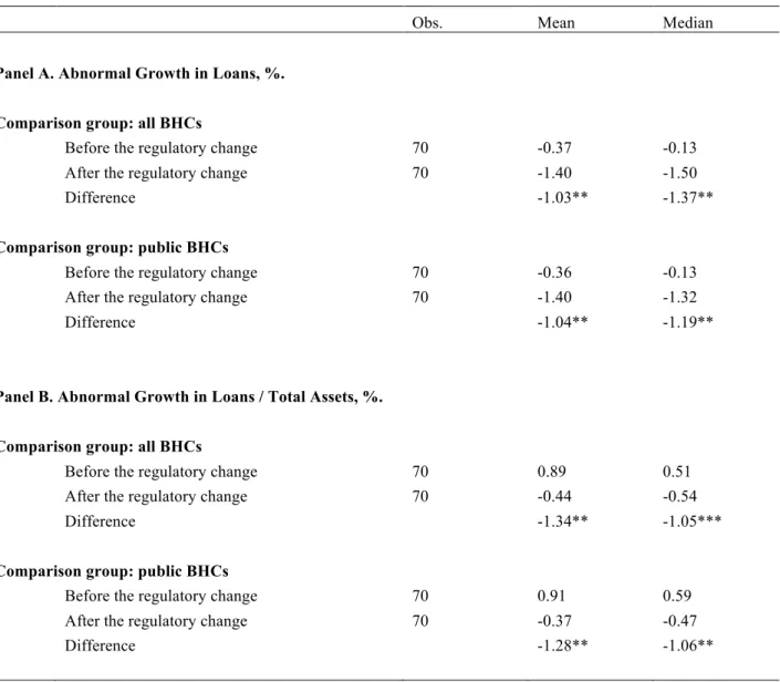
Panel A of Table 2 shows that the average abnormal growth rate in loans for dealer banks
declined in the four quarters after the regulatory change compared to the four quarters before.
The magnitude of the decline in abnormal loan growth rate (-1.03%) is economically significant
compared to the average growth rate of 2.5% in the total sample during this period. Analysis of
medians leads to a similar conclusion: the regulatory change of July 1996 was followed by a
statistically and economically significant decline in the loan growth rate. The magnitude of the
median decline is large compared to the median growth rate of loans (2.2%) in the total sample
during this period. This result holds if the subsample of public bank holding companies is used
as a comparison group of banks, as shown in the second half of Panel A of Table 2.
To ensure that the negative abnormal growth in loans does not simply reflect changes in total
difference-in-difference test for the changes in the ratio of loans to total assets. Panel B of Table 2 shows that
when measured this way, loans at dealer banks declined after the regulatory change in both
means and medians.
I also conduct a regression analysis of changes in loan growth at dealer banks to ensure that
the decline in means and medians is not driven by other bank characteristics. As with the
univariate tests, I restrict the sample to the time period starting four quarters before and ending
four quarters after the July 1996 change in the revenue limit. An indicator variable Post 1996 is
defined for four quarters after the regulatory change. An indicator variable Dealer is defined for
the group of banks that established Section 20 subsidiaries as of June 30, 1995. The major
coefficient of interest in this regression is the interaction term of these two indicator variables
Post 1996 * Dealer.
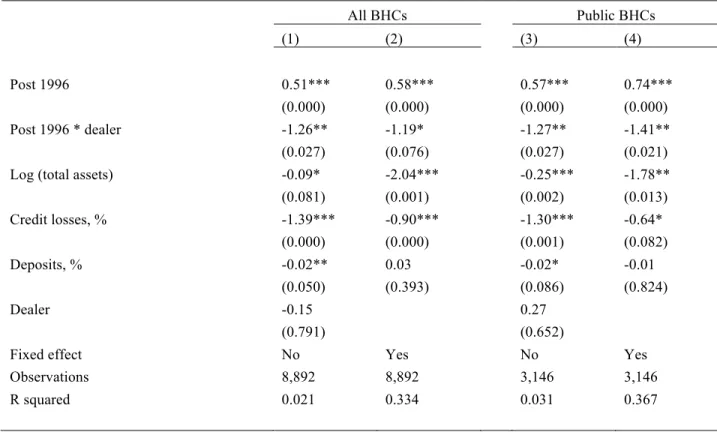
In column 1 of Table 3 the coefficient before the interaction term Post 1996 * Dealer is
negative and statistically significant at 5%. This suggests that even after controlling for other
bank characteristics, dealer banks had a lower growth rate in loans than non-dealer banks. At the
same time, the growth rate in loans in the total sample is positive, as suggested by the positive
coefficient on the indicator Post 1996. Larger banks have on average lower growth rate in loans.
As one would expect, banks with more credit losses tend to increase their loan portfolio more
slowly. In column 2 I include bank fixed effect to control for any time-invariant omitted
variables. The coefficient for the interaction term Post 1996 * Dealer remains significant at 10%,
and has similar magnitude. Both magnitudes are close to the mean and median abnormal growth
rates from the univariate tests. In columns 3 and 4 I repeat the regressions for a smaller
I also conduct a similar test for the regulatory change in 1989. However, I do not find a
similar effect there. This could be for the reasons explained above (the majority of Section 20
subsidiaries were established between 1987 and 1989 and the magnitude of increase in the
threshold in 1989 was small relative to that of 1996).
3.5 Aggregate lending implications of the regulatory change of 1996
Although we find that abnormal loan growth rates of dealer banks declined after the
regulatory change of 1996 compared those of non-dealers, it is likely that borrowers rejected by
dealer banks received loans from non-dealer banks competing in the same geographic region.
However, this substitution may be incomplete. To estimate the net effect of the regulatory
change on lending, the dollar amounts of growth in loan balances (rather than percentages) for
dealer and non-dealer banks are summed up as follows:
∑
∑
∑
∑
∑
∑
= − − = = = − − = = ⎟ ⎠ ⎞ ⎜ ⎝ ⎛ Δ − Δ + ⎟ ⎠ ⎞ ⎜ ⎝ ⎛ Δ − Δ = D j t j t t j t ND i t i t t it L L L
L 1 4 1 4 1 1 4 1 4 1 Change Lending Aggregate
where ND – the number of non-dealer banks
D – the number of dealer banks
i
t
L
Δ – change in loan balances at a bank i in quarter t (in $)
In the subsample of public banks only, the total effect of the regulatory change on lending
growth is estimated to be -$20 billion. In the sample of all bank holding companies it is $2.5
billion. None of private banks in the sample are dealers, and showed a positive change in average
growth rate in loan balances, so compensating for the negative effect at public banks. These
of total lending. In other words, when measured in dollar terms rather than in percentages, the
conclusions are quite different. This might be explained by the fact that banks of different size
had different growth rates in loans.
3.6 What drives reduction in loan growth: demand or supply?
Another interesting/important question is whether this change is driven by lower loan
demand or tighter loan supply. As a way to disentangle these two effects I look at more detailed
data on mortgage loan applications. This data makes it possible to model the probability of an
application being denied by a bank, controlling for borrower, lender and geographic area
characteristics. This has two purposes. First, mortgage application denial rates capture the supply
side of lending, i.e. the willingness of lenders to make loans. Examining mortgage application
denial rates, I can ensure that the decline in loan growth rates documented in the previous tables
is not driven by a decline in demand. Second, this provides an independent robustness check of
the result documented using aggregate amounts of loans from bank financial statements.
HMDA data on mortgage applications is matched to the major dataset by the name and state
of banks that are included in a Bank Holding Company. Linear probability models are estimated
despite the fact that the dependent variable is an indicator variable, for which a probit model
seems to be more suitable following Puri, Rocholl and Steffen (2011). The major reason for
using this approach is that bank fixed effect should be included in these regressions to remove
the effect of time-invariant omitted variables and alleviate the endogeneity problem. However,
nonlinear models suffer from an incidental parameter problem, i.e. the fixed effects and the
(with the number of time periods fixed and the number of groups growing infinitely).2 In
contrast, in linear models the coefficients of the main explanatory variables can be estimated
consistently. The results are robust to using logit as an alternative estimation method, as
described below in more detail.
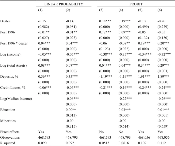
Columns 1 and 2 of Panel A in Table 4 show the estimates of the linear probability models
for the subsample of public banks. The sample period includes one year before and after the
regulatory change of July 1996 (1995 and 1997). The dependent variable is set to one if a
mortgage application was rejected by a bank and to zero if the loan was granted. The interaction
term between the indicator for the Section 20 bank and the indicator for the period after the
regulatory change of 1996 is positive and significant at 1% level. The denial rate of mortgage
applications at these banks increased after the regulatory change. In other words, mortgage
underwriting standards at these banks became stricter. This is consistent with lower loan growth
rates in the tests that used data on loans from bank financial statements. The magnitude of the
effect is significant not only statistically but also economically. After the regulatory change,
dealer banks had a 6% higher denial rate. It is almost one quarter of the average denial rate in the
sample of 29%.
In these regressions I control for a few applicant, bank and geographic area characteristics.
As a measure of creditworthiness, applicant income is used. Although this is only one component
of the credit scores typically used as a proxy for creditworthiness, credit score data is
unfortunately prohibitively expensive. The coefficient before the logarithm of applicant income
is negative and significant in all specifications. This is consistent with the intuition that higher
2 Neyman and Scott (1948) show that the incidental parameters (fixed effects) become inconsistent in logit models
income applicants have higher chances of being approved for a mortgage loan. Banks with a
higher fraction of assets financed by deposits have higher denial rates. This result might reflect
the conservativeness of a bank in both lending and funding. In column 2 a number of
demographic characteristics of the geographic region in which an applicant lives are added.
These are considered at the county level. The signs of the coefficients for these variables are
consistent with expectations; applicants living in the counties with higher than average
household income have lower denial rates, while those in the counties with a higher percentage
of residents educated to less than college level have higher denial rates.
Fitting a linear probability model for an indicator variable can be questioned because it can
predict values that are negative or outside the range (0;1). For this reason, probit specifications
are commonly used to model binary data. However, as discussed above, linear probability model
has an important advantage for panel data. In contrast to a probit model, it provides consistent
estimates of the main explanatory variables in models with firm fixed effects. As a robustness
check of the previous result, the coefficients for probit models with and without bank fixed
effects are shown in columns 3–6. The interaction terms between the dealer bank indicator and
the indicator for the post-1996 period as well as control variables retain their sign and
significance in all four specifications.
To get a better comparison group for the group of banks under study, I also estimate separate
models for the probability of mortgage denial for the ten largest US states. Banks operating in
the same state are subject to similar economic and demographic conditions, as well as the same
regulation. For example, whether a mortgage is no-recourse, so that the bank does not pursue a
borrower to get the difference between the amount of the mortgage and the value of the house in
Table 4 is used to fit linear probability models with bank fixed effects for each state. Panel B of
Table 4 shows the estimates of the coefficients before the interaction term between the
bank-dealer indicator and Post 1996 indicator. Eight out of ten states have positive and statistically
significant coefficients for this interaction term. The fact that bank-dealer denial rates did not
increase in California can be explained by the fact that many Internet and high-tech companies
are located there and that 1997 was a year of the Dotcom boom.
Finally, as an additional robustness check, loan level HMDA data is aggregated up to the
bank level and linear regression models for bank average denial rate on mortgage applications
for a given year is fit. Coefficients of this estimation are shown in Panel C of Table 4. They
confirm the results obtained above for both all bank holding companies and the subsample of
public ones only: dealer banks were more likely to deny mortgage applications after the 1996
regulatory change.
3.7 Which types of borrowers experience a reduction in credit availability?
It is not obvious which types of borrowers experienced most of the reduction in credit
availability after the change in regulation: those who were more or less creditworthy. Less
creditworthy borrowers can be charged a higher interest rate, although such loans might lead to
larger expected losses. To choose the optimal mix of loans, a bank needs to evaluate the
risk-return tradeoff. Borrower creditworthiness is usually measured by credit scores. However, the
HMDA dataset does not include this variable. To overcome this data limitation, borrower income
reported in HMDA is used.
The total sample is split into two parts: borrowers with higher and lower than the median
these two subsamples. Most importantly, the interaction term Post 96 * Dealer has significantly
positive coefficients in both subsamples (except for the probit models without fixed effects in the
subsample of high-income borrowers). This suggests that both groups of borrowers were affected
by the regulatory changes. As might be expected, the magnitude of the effect was slightly greater
for low-income borrowers. However, an important limitation of this analysis is that this
conclusion is based on a specific measurement (income) that is only one component of the credit
scores that are typically used by measure borrower creditworthiness.
3.8 Alternative explanations
It is reasonable to suggest that Section 20 banks securitized a large fraction of their loans and
that the fraction of loans they securitized went up over time. Even if the amount of all originated
loans was not affected, increase in the extent of securitization resulted in the reduction of the
growth rate for loans held on bank balance sheets. To rule out this alternative explanation, the
dynamics of securitization rates around 1996 at dealer and non-dealer banks need to be
compared. HMDA mortgage loan data includes information about whether a loan was kept by a
bank on its balance sheet or sold after the origination into securitization pools. An indicator for
securitization is defined on the basis of this information.
Table 5 shows the estimates of linear regression models with the percentage of all granted
loans being securitized or sold by the originator in a given year as a dependent variable. The
sample period includes one year before and after the regulatory change of July 1996. The
interaction term between the indicator for the Section 20 bank and that for the period after the
regulatory change of 1996 is negative and significant at a level of 10%. This means that the
down in 1997. This suggests that the lower growth rate in dealer banks after the regulatory
change was not due to higher securitization rates at these banks.
4. Exogenous Shock II: Intensified Capital Market Frictions during Periods of High Uncertainty
4.1. Incentives in market-making during periods of high uncertainty
As discussed in the first part, when market-making and lending are combined in one
financial institution, they compete for funding, so that such financial institutions exhibit different
lending patterns than others. To study these spillover effects in a time series context, I consider
periods when uncertainty about the future increases exogenously. It is reasonable to expect that
capital market frictions intensify at these periods. The effect of market-making on lending may
therefore be particularly pronounced because it becomes especially difficult for a bank to raise
new financing on capital markets. And it is during these periods that market-making by a
financial institution may have particularly pronounced effects on its lending.
However, it is important to note that intensified capital market frictions form a necessary,
though not a sufficient, condition for market-making to affect lending. It is crucial that the bank
headquarters have incentives to redistribute funding away from lending towards market-making.
There are a number of arguments why the demand for market-making is likely to change during
periods of high uncertainty, and how this change affects the incentives of the market-making
division. Asset pricing literature suggests that at periods of high uncertainty on capital markets,
demand for market-making is particularly strong. After negative shocks to the markets it is
common to observe so called flight to quality, in which investors sell riskier assets and buy
liquidity provision increases at these periods, and selling pressure is further amplified by a
number of frictions discussed in asset pricing literature. Traders liquidate positions across
different securities after trading losses (Kyle & Xiong, 2001). When fund performance falls
below a threshold, fund managers are subject to withdrawals (Vayanos, 2004). Increase in
hedging demands by investors is another reason for the increase in trading volume. In addition to
these mostly theoretical arguments, there are also evidence of a positive relation between
volatility and trading volume in the empirical asset pricing literature. Gallant, Rossi and Tauchen
(1992) show that large price movements in equity prices are followed by high volume. Fleming
(2003) reports positive time series correlation between volatility and trading volume for US
Treasuries, which make up the largest segment of bond markets in terms of trading activity
(according to FISMA, Treasuries represent about 60% of trading volume in all bonds). Foster
(1995) finds that volatility and volume in the oil futures markets are positively
contemporaneously related. Wang and Yau (2000) find positive relation between volatility and
trading volume for futures on S&P 500, Deutsche Mark, silver and gold.3
As a consequence of increased demand, return on liquidity provision increases during
periods of high uncertainty. Dealers set wider bid-ask spreads to compensate for the increase in
inventory risk borne by a market-maker (Ho & Stoll, 1983). Nagel (2011) shows that return from
reversal strategies is higher when VIX is higher. Fleming (2003) finds a positive correlation
between price volatility and bid-ask spreads in US Treasuries. Chordia, Sarkar and
Subrahmanyam (2005) find that volatility is informative in predicting bid-ask spreads for stocks
3 In addition to the findings of the previous literature in undocumented results I show that if I use our specific
and US Treasuries. Wang and Yau (2000) document a positive relation between volatility and
bid-ask spread for a number of futures (S&P 500, Deutsche Mark, silver and gold).
Because the demand for liquidity provision on capital markets increases at periods of
high uncertainty, shifting funds from lending to this activity is a feasible and likely strategy for
dealer banks. It is important to acknowledge, however, that at these periods the risks of
market-making also increase.
I describe the empirical evidence consistent with this hypothesis below. Most
importantly, at the periods of high uncertainty the following holds for dealer banks: (1) higher
risk-adjusted trading returns; (2) increase in trading assets; (3) decline in loan growth rate
compared to non-dealers. High uncertainty periods are defined as quarters when the average
daily VIX is in the top 25% for the period from the beginning of the series in 1990 until 2008. As
a robustness check, I also use a 20% cutoff. The list of high-volatility quarters for 25% cutoff
includes the following events:
§ Asian crisis (Q7, 1997)
§ LTCM (Q3 1998–Q3 1999)
§ Dotcom bubble (Q3 2000–Q4 2001)
§ Worldcom bankruptcy (Q3 2002–Q1 2003)
§ Subprime crisis (Q1, Q3–Q4 2008)
Hypothesis II
At the periods of high volatility dealer banks shift funds away from lending to market making
because of increased demand for market making.
4.2. Trading returns and trading assets of dealer banks in high uncertainty periods
To provide evidence on the second hypothesis about bank incentives switching from
lending to market making during the high uncertainty periods, I compare the risk-adjusted gross
trading returns of dealer banks in high- and low-volatility quarters. Two measures of trading
returns are used. Marked-to-Market Risk-Adjusted Return, % is the ratio that has in the
numerator trading revenues per $1 of trading assets (the ratio of marked-to-market trading
revenues [item BHCK A220] to the amount of trading assets at the beginning of the quarter). The
denominator adjusts for risk to account for the fact that dealers might be compensated by higher
returns for taking more risk at the periods of high volatility. As a measure of riskiness of trading
assets I use Value at Risk (VaR) [item BHCK 1651] per unit of trading assets that all banks with
a trading position exceeding $1 billion or 10% of total assets are required to report. As a result, I
get a measure similar to the Sharpe ratio by dividing trading revenue per $1 of trading assets by
VaR per $1 of trading assets. Another measure, Total Risk-Adjusted Return, %, includes not only
marked-to-market trading revenue, but also interest income from trading assets [BHCK 4069].
The sum of these two types of revenue per $1 of trading assets is divided by VaR per $1 of
trading assets to get the second measure of trading returns. Because of the limited information
provided in BHC financial statements it is possible to calculate only gross returns, which do not
take into account the costs of trading (most importantly funding costs and overhead expenses).
Panel A of Table 6 shows that both measures of gross risk-adjusted trading returns at
dealer banks are higher in high volatility periods than in low volatility periods. The difference in
marked-to-market returns is statistically significant at 5% and economically large (mean: 1.2%,
median: 0.74%) compared to the level of gross trading returns at low-volatility periods (mean:
total returns between high- and low-volatility periods is statistically significant at 1% level and
economically large (mean: 1.42%, median: 2.27%) compared to the level of total returns at
low-volatility periods (mean: 6.23%, median: 4.43%). The right side of Panel A of Table 4 shows that
the result is robust to the change in cutoff for a definition of high-volatility periods, although
statistical significance is weaker, perhaps because of the smaller number of observations in the
high-volatility subsample. These results suggest that dealer banks do have incentives to shift
funds to market-making during high-uncertainty periods because they receive higher
risk-adjusted trading returns at such times.
I also examine empirically whether dealer banks shift funds to market-making. First, I
consider whether dealer banks increase their trading- to total-assets ratio during high-volatility
quarters. Since trading assets can be rather volatile, I use the average trading- to total-assets ratio
in the previous four quarters as a benchmark for comparison. I calculate Abnormal Trading
Assets, % as a percentage change in the ratio of trading assets to total assets relative to the bank
average in the previous four quarters.
Panel B of Table 6 shows that although trading assets were growing even during
low-volatility quarters, their average growth was significantly faster during high-low-volatility quarters.
The difference is statistically significant at 1% level for both mean and median. This result also
holds if the cutoff for high-volatility quarters is moved to 20% from 25%, as shown on the right
side of Panel B in Table 6. This suggests that dealer banks do move funds to market-making
during high-uncertainty periods.
Some trading assets are often financed with trading liabilities that include short positions
allocate equity capital for the gross amount of trading assets rather than trading assets net of
liabilities. Since equity capital is the most expensive form of funding, there is therefore the
greatest competition to obtain it. Consequently, in our tests focused on competition between
bank divisions for equity capital, it makes sense to consider changes in total rather than net
trading assets.
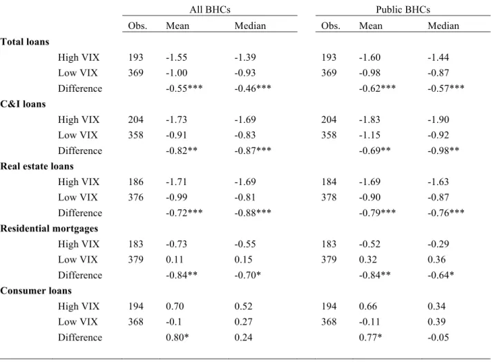
4.3. Lending by dealer banks during high-uncertainty periods
To study the effect of market-making on lending during periods of high volatility, I
perform a difference-in-difference test for the growth rates in loans. For each quarter I calculate
abnormal loan growth rates at dealer banks relative to non-dealers. I use two different
comparison groups: all bank holding companies and public only bank holding companies. Then I
compare abnormal loan growth rates for dealer banks at high- and low-volatility periods. Table 7
shows that abnormal growth rates of loans were lower during high-volatility quarters than in
low-volatility quarters. For all loans, the difference is statistically significant at 1% level. The
magnitude of the average difference (-0.55%) is economically large. It is about half of the
abnormal total loan growth rate for dealer banks during low-volatility periods (-1.0%) and about
one fifth of the unadjusted loan growth rate in the total sample (2.5%). Similar conclusions can
be made based on medians and with public BHCs used as a comparison group. The result holds
for three out of four types of loans (corporate, residential and non-residential loans) considered
separately.
In Table 8 I conduct a multivariate analysis to ensure that lower loan growth rates at
dealer banks in periods of high uncertainty are not driven by other bank characteristics. The
with the indicator for dealer-banks High VIX * Dealer. In all four specifications of Table 8, this
interaction term is significantly negative at 5% level. This suggests that even after controlling for
other bank characteristics, dealer banks have a lower loan growth rate relative to non-dealer
banks during periods of high uncertainty. The magnitude of the effect is similar to the magnitude
in the univariate tests.
The coefficients on other variables are consistent with expectations. Larger banks tend to
have slower growth rates. Banks using more deposit financing and borrowing less on capital
markets grow slower. Banks with higher credit losses are more conservative in lending and
increase their loans more slowly.
4.4. Alternative explanations
Periods of high uncertainty are often (although not always) accompanied by recession in
the real economy. For example, the LTCM crisis of 1998 did not lead to a recession in the US,
although it caused a lot of turbulence on the financial markets, while high volatility in the capital
markets in 2001 was accompanied by a recession. Previous literature has suggested mechanisms
that can propagate financial shocks to generate recession in the real sector. One of them is the
financial accelerator introduced by Bernanke and Gertler (1989) and Kiyotaki and Moore (1997).
The major transmission channel in these models is the increase in agency costs of borrowing
after a negative financial shock, leading to a reduction in borrower net worth or collateral. It is
therefore important to ensure that lower loan growth at dealer banks during high-volatility
periods is not simply driven by an overlap between high-volatility and recession quarters.
To study this question, I define an indicator variable NBER Recession for the quarters
1996–2008, includes two recessions: those of 2001 (from the second to the fourth quarter) and
2008 (all four quarters). I also define the interaction of this indicator with the indicator for dealer
banks. Comparison of column 2 with column 1 of Table 9 shows that the decline in lending by
public banks was twice as large during the recessions. However, the interaction term High VIX *
Dealer remains negative and significant, suggesting that lower growth in loans during
high-volatility periods is not driven by overlaps with recessions.
Another concern one might have regarding the findings in this thesis is that dealer banks
tend to rely on borrowing from capital markets as a source of funding, and it could be this
funding difficulty (rather than presence of market-making divisions) that explains the reduction
in lending by dealer banks during periods of high volatility. To rule out this alternative
explanation, I include the interaction of the indicator for high-volatility periods and a variable
characterizing the composition of bank financing. For this purpose I define two variables:
percentage of deposit financing; and percentage of non-deposit borrowings including interbank
loans, REPO, commercial papers, bonds, etc. Columns 3 and 4 of Table 9 show that even after
inclusion of these interaction terms, the coefficient before High VIX * Dealer remains
significantly negative. This suggests that non-dealer banks that borrow on capital markets do not
reduce their lending at times of high volatility more than other banks, and our result is not driven
only by difficulties in financing at dealer-banks during high-volatility periods. However, as is
discussed above, difficulty in obtaining external financing is a necessary condition for internal
5. Conclusion
In this thesis I study the patterns of lending within financial institutions that combine
mortgage lending with making markets in securities. In order to address the causality concerns,
two exogenous shocks were used. In Section 3.3 it was shown that after the regulatory change of
1996 affected dealer banks reduced their lending and rejected a larger portion of mortgage
applications. In Section 4.2 it was demonstrated that during periods of high uncertainty on capital
markets, dealer banks have incentives to shift funds away from lending and towards market
making because of the higher demand for liquidity provision at such times. The major
implication of these findings is that an increase in market making at a commercial bank can
reduce loan growth, and that this effect is particularly pronounced during the high volatility
Appendix A. Commercial Banks – Dealers in Securities
This table shows the list of bank holding companies that had established Section 20 subsidiaries to underwrite and deal in securities as of June 30,1995.
Bank Holding Company Name 1 Banc One Corp.
2 Bank of Boston Corp. 3 Bank South Corp. 4 BankAmerica Corp. 5 Barnett Banks, Inc. 6 Chase Manhattan Corp. 7 Chemical New York Corp. 8 Citicorp
9 CoreStates Financial Corp. 10 Dauphin Deposit Corp. 11 First Chicago Corp. 12 First Interstate Bancorp 13 First of America Bank Corp. 14 First Union Corp.
15 Fleet/Norstar Financial Group, Inc. 16 Huntington Bancshares, Inc. 17 JP Morgan & Co., Inc. 18 Key Corp
19 Mellon Bank Corp. 20 National City Corp.
21 NCNB Corp. (later NationsBank) 22 Norwest Corp.
Table 1. Summary Statistics for Dealer Banks.
Loan Growth Rate, % is the quarterly growth rates in bank loan balances at dealer banks in 1995–2008. All other
bank characteristics are reported as of June 30, 1995. Credit Losses, % are charge-offs on loans expressed as a percentage of total loans on bank balance sheet.
Mean Median
Loan growth, % 1.07% 1.23%
Total assets, $billion 81.7 66.6
Loans, % total assets 62.3 67.1
Trading assets, % total assets 5.3 0.3 Credit losses, % total loans 0.11 0.11 Deposits, % total assets 57.3 62.3
Table 2. Loan Growth at Dealer Banks after the Regulatory Change I: Difference-in-Difference Tests.
Panel A shows abnormal quarterly growth rates in bank loan balances (in %) at dealer banks four quarters before and after the regulatory changes of July, 1996. Panel B shows abnormal quarterly growth rates in loans to total assets ratios at dealer banks four quarters before and after the regulatory changes of July, 1996. ***, ** and * indicate statistical significance at the 1%, 5% and 10% level, respectively.
Obs. Mean Median
Panel A. Abnormal Growth in Loans, %.
Comparison group: all BHCs
Before the regulatory change 70 -0.37 -0.13 After the regulatory change 70 -1.40 -1.50
Difference -1.03** -1.37**
Comparison group: public BHCs
Before the regulatory change 70 -0.36 -0.13 After the regulatory change 70 -1.40 -1.32
Difference -1.04** -1.19**
Panel B. Abnormal Growth in Loans / Total Assets, %.
Comparison group: all BHCs
Before the regulatory change 70 0.89 0.51 After the regulatory change 70 -0.44 -0.54
Difference -1.34** -1.05***
Comparison group: public BHCs
Before the regulatory change 70 0.91 0.59 After the regulatory change 70 -0.37 -0.47
Difference -1.28** -1.06**
Table 3. Decline in Loan Growth at Dealer Banks after the Regulatory Change II: Regression Analysis.
This table shows estimates of the coefficients for OLS regressions with quarterly growth rates in bank loan balances (%) as dependent variables. Sample period includes four quarters before and four quarters after the regulatory change of July 1996. Post 1996 is an indicator variable for four quarters after the regulatory change. Dealer is an indicator variable for banks that established Section 20 subsidiaries as of the end of the second quarter of 1995.
Credit Losses, % are charge-offs on loans expressed as a percentage of total loans on bank balance sheet. ***, **
and * indicate statistical significance at the 1%, 5% and 10% level, respectively. p-values based on heteroskedasticity-adjusted and clustered by bank standard errors are reported in parenthesis.
All BHCs Public BHCs
(1) (2) (3) (4) Post 1996 0.51*** 0.58*** 0.57*** 0.74***
(0.000) (0.000) (0.000) (0.000) Post 1996 * dealer -1.26** -1.19* -1.27** -1.41**
(0.027) (0.076) (0.027) (0.021) Log (total assets) -0.09* -2.04*** -0.25*** -1.78**
(0.081) (0.001) (0.002) (0.013) Credit losses, % -1.39*** -0.90*** -1.30*** -0.64*
(0.000) (0.000) (0.001) (0.082) Deposits, % -0.02** 0.03 -0.02* -0.01
(0.050) (0.393) (0.086) (0.824)
Dealer -0.15 0.27
(0.791) (0.652)
Fixed effect No Yes No Yes
Observations 8,892 8,892 3,146 3,146 R squared 0.021 0.334 0.031 0.367
Table 4. Mortgage Application Denial Rates at Dealer Banks after the Regulatory Change
Panel A shows estimates of the linear probability models and probit models with the dependent variable equal to one if a mortgage application is denied by a bank and to zero if the loan is granted. Panel B reports coefficients of the interaction terms for linear probability models estimated separately for ten US states with the largest population. Control variables are the same as in the specification (2) of Panel A. Sample used in panels A and B includes only public bank holding companies and covers one year before and after the regulatory change of July 1996 (1995 and 1997). Panel C shows estimates of OLS regressions with the bank average mortgage application denial rate as dependent variables. Post 1996 is an indicator variable for 1997, the year after the regulatory change. Dealer is an indicator variable for banks that established Section 20 subsidiaries before 1995. Credit Losses, % are charge-offs on loans expressed as a percentage of total loans on bank’s balance sheet. Median Income is the logarithm of the median household income in a county. Education is the percentage of population in the county with high school education. Minorities is the percentage of non-white population in a county. ***, ** and * indicate statistical significance at the 1%, 5% and 10% level, respectively. p-values based on heteroskedasticity-adjusted and clustered by census tract standard errors are reported in parenthesis.
Panel A. Probability of Mortgage Application Denial
LINEAR PROBABILITY PROBIT
(1) (2) (3) (4) (5) (6)
Post 1996 0.00 0.00 0.21*** 0.18*** 0.03 0.03 (0.929) (0.973) (0.000) (0.000) (0.209) (0.266) Dealer -0.38 -0.39 0.21*** 0.22*** 0.32 0.09
(0.876) (0.989) (0.000) (0.000) (0.337) (0.681) Post 1996 * dealer 0.06*** 0.06*** 0.15*** 0.10*** 0.24*** 0.24***
(0.000) (0.000) (0.000) (0.003) (0.000) (0.000) Log (income) -0.13*** -0.12*** -0.70*** -0.65*** -0.57*** -0.55***
(0.000) (0.000) (0.000) (0.000) (0.000) (0.000) Log (total assets) 0.06*** 0.05*** 0.01 0.01 0.12 0.10
(0.004) (0.010) (0.445) (0.338) (0.119) (0.198) Deposits, % 0.54*** 0.53*** -1.50*** -1.41*** 2.04*** 2.05***
(0.000) (0.000) (0.000) (0.000) (0.000) (0.000) Credit losses, % -0.09*** -0.09*** -0.52*** -0.44*** -0.29*** -0.29***
(0.000) (0.000) (0.000) (0.000) (0.000) (0.000) Log (median income) -0.06*** -0.24*** -0.12**
(0.000) (0.000) (0.023) Education 0.00* 0.02*** 0.01***
(0.083) (0.000) (0.005) Minorities -0.00 -0.00 0.00
(0.734) (0.870) (0.456) Fixed effect Yes Yes No No Yes Yes Observations 915,982 915,982 915,982 915,982 915,719 915,719
R squared 0.238 0.239 0.155 0.164 0.222 0.223
Panel B. Probability of Mortgage Application Denial for 10 US States
State Post 1996 * Dealer p-value
Observations (Number of applications)
R-squared
1 California -0.02 (0.521) 54,413 0.090 2 Florida 0.11** (0.018) 87,911 0.091 3 Georgia -0.08*** (0.009) 35,595 0.460 4 Illinois 0.14*** (0.000) 19,217 0.111 5 Michigan 0.28*** (0.000) 35,096 0.207 6 New York 0.09*** (0.007) 42,075 0.198 7 North Carolina 0.09* (0.085) 56,049 0.408 8 Ohio 0.05*** (0.000) 50,867 0.208 9 Pennsylvania 0.10*** (0.000) 41,736 0.188 10 Texas 0.12*** (0.003) 37,839 0.184
Panel C. Determinants of the Bank’s Average Mortgage Application Denial Rate
All BHCs Public BHCs
(1) (2) (3) (4)
Post 1996 -0.01 -0.00 0.01* 0.01** (0.127) (0.497) (0.087) (0.036)
Dealer 0.05 0.05 0.03 0.04
(0.102) (0.124) (0.224) (0.208) Post 1996 * Dealer 0.09*** 0.09*** 0.07** 0.07** (0.008) (0.006) (0.045) (0.031) Log(Total Assets) 0.02*** 0.02*** 0.03*** 0.02***
(0.000) (0.000) (0.000) (0.000) Deposits, % 0.15** 0.09* 0.21** 0.11
(0.016) (0.062) (0.019) (0.115) Credit Losses, % 0.01 0.02* -0.00 0.00
(0.209) (0.090) (0.883) (0.579) Log(Av. Income) -0.06*** -0.07***