An Investigation of Humeral Stress Fractures in Racing Thoroughbreds using a 3D Finite Element Model in Conjunction with a Bone Remodeling Algorithm
A Thesis presented to
the Faculty of California Polytechnic State University,
San Luis Obispo
In Partial Fulfillment
of the Requirements for the Degree
Master of Science in Biomedical Engineering
by
Ryan James Moore
iii
COMMITTEE MEMBERSHIP
TITLE: An Investigation of Humeral Stress Fractures in Racing
Thoroughbreds using a 3D Finite Element Model in
Conjunction with a Bone Remodeling Algorithm
AUTHOR: Ryan James Moore
DATE SUBMITTED: February 26, 2010
COMMITTEE CHAIR: Scott Hazelwood, Associate Professor
COMMITTEE MEMBER: Lanny Griffin, Department Chair
iv ABSTRACT
An Investigation of Humeral Stress Fractures in Racing Thoroughbreds using a 3D Finite Element Model in Conjunction with a Bone Remodeling Algorithm
Ryan James Moore
The humerus of a racing horse Thoroughbred is highly susceptible to stress fractures at a characteristic location as a result of cyclic loading. The propensity of a Thoroughbred to exhibit humeral fracture has made equines useful models in the epidemiology of stress fractures. In this study, a racing Thoroughbred humerus was simulated during training using a 3D finite element model in conjunction with a bone remodeling algorithm. Nine muscle forces and two contact forces were applied to the 3-dimensional finite element model, which contains four separate load cases representing fore-stance, mid-stance, aft-stance, and standing. Four different training programs were incorporated into the model, which represent Baseline Layup and Long Layup training programs along with two newly implemented programs for racing, which have an absence of a layup period, last a period of 24 weeks, and a race once every four weeks. Muscle and contact forces were rescaled for all load cases to simulate dirt, turf, and synthetic track surfaces. Bone porosity, damage, and BMU activation frequency were examined at the stress fracture site and compared with a control location called the caudal diaphysis. It was found that race programs exhibited similar remodeling patterns
v
ACKNOWLEDGMENTS
This project was made possible through collaborations with California Polytechnic State
University San Luis Obispo and the University of California at Davis. Funding was
provided by the NIH (National Institutes of Health). I would like to thank my thesis
project advisor Dr. Scott Hazelwood for his guidance and assistance throughout the
project. I would also like to thank my parents Steven and Linda for support during my
vi
TABLE OF CONTENTS
Page
LIST OF TABLES ………...……… vii
LIST OF FIGURES ...……….……... ix
CHAPTER I. INTRODUCTION ………... 1
Thoroughbred Race Horse Injuries ………... 1
The Characteristics, Function, and Biology of Bone ………. 3
Stress Fractures ……….. 13
Finite Element Analysis ………... 16
Bone Remodeling Algorithm ………... 18
Layup Training Programs and Race Programs……… 20
Goals and Hypotheses ………. 22
II. METHODS ………. 23
Development of Finite Element Model ...……….…….. 23
Contact and Muscle Forces …………...………. 25
Remodeling Algorithm ………... 32
Creation of Equilibrium Model ………...………. 36
Rescaling Forces for Turf and Synthetic Tracks ………. 39
Training Programs ………... 43
III. RESULTS ……… 49
Equilibrium Model and Remodeling Parameters ………. 49
Baseline Layup Training Program ……….……….. 51
Long Layup Training Program ……….... 52
Model Validation (Hypothesis 1) ……… 53
Race Programs ……….…….57
Effects of Turf and Synthetic Tracks on Bone Remodeling ……… 61
IV. DISCUSSION ……….. 74
Bone Response and Remodeling ………. 74
Race Programs (Hypothesis 2) ……… 78
Turf and Synthetic Track Surfaces (Hypothesis 3) ……….. 80
Limitations and Future Updates ………... 84
Project Summary ………... 86
vii
LIST OF TABLES
Table Page 1. Anisotropic data from a bovine and human bone (Reilly et al., 1974; Reilly and
Burstein, 1975) .…………....………... 12
2. EMG walking data from an equine (Korsgaard, 1982) and a canine (Tokuriki, 1973). Canine EMG data ranged from 0 to 5, where 0 represents no activity and 5 corresponds to abundant activity. N/A indicates a lack of EMG data….. 28
3. Canine EMG data attached to the proximal humerus during gallop. An
activation level of 5 corresponds to the highest EMG activity, while a level of 0 corresponds to no EMG activity (Tokuriki, 1973)……….. . 28
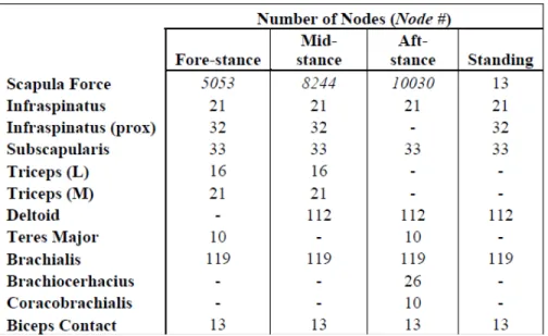
4. Number of nodes applied per force applied over a specific area during the gait cycle and standing. Italics for the scapula force represent the node
number of forces applied at a single node (Ferullo, 2007) ………..……… 29 5. Locations (mm) of muscle and contact forces for the humeral (Coordinate 1)
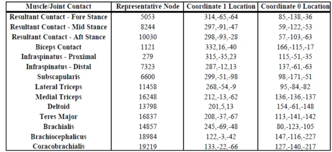
and global (Coordinate 0) coordinate systems. The representative node is the center of the area for forces applied over more than one node (Ferullo, 2007) ... 30 6. Initial values for state variables used in the bone remodeling algorithm
(Hazelwood et al., 2001) ……….. 33 7. Constants used in the remodeling simulation. Loading rates are given in
cycles per day (Ferullo, 2007) ………. 33
8. Muscle and contact forces components during the standing load case used in the FEA input file for dirt (Ferullo, 2007), turf, and synthetic tracks. Dirt track values were previously adjusted from a range of literature to fit an
accurate physiological porosity distribution (Ferullo, 2007) ………... 38
9. Dirt track muscle and contact force components during the three separate phases of walking placed in the FEA input file. These forces were increased by a factor of 2.8 and 3.5 within the algorithm to simulate slow and fast
galloping speeds, respectively (Ferullo, 2007) ………..….. 38 10. Scaled down muscle and contact force components for the turf track during
the three phases of walking ……….. 42
11. Scaled down muscle and contact force components for the synthetic track during the three phases of walking ……….. 42 12. Baseline Layup training program with 8 weeks of layup. Distances are given in
miles, furlongs, and number of strides during the high speed exercise
viii
LIST OF TABLES
Table Page 13. Long Layup training program with 16 weeks of layup. Distances are given
in miles, furlongs, and number of strides during the high speed exercise
completed on day 6 (Ferullo, 2007) ………. 46
14. Comparison of the first four weeks of race training for the race programs ……. 47 15. Race Program 1 with no extended period of layup. High speed gallop and
race distances are given in miles, furlongs, and number of strides. Races occur once every four weeks during the race training period of the program …. 48 16. Race Program 2 with no extended period of layup. High speed gallop and
ix
LIST OF FIGURES
Figure Page
1. Sketch of typical long bone features (Martin et al., 1998) ………. 5 2. Illustration of the creation of a secondary osteon through the resorption of
osteoclasts followed by osteoblasts, which are forming new bone to establish a newly remodeled haversian system (Nunamaker, 2002a) ………. 10 3. Microradiograph of remodeling in horse bone within the cortex. The larger
black areas represent resorption cavities, while the grey oval shaped areas represent new-less calcified bone making up secondary osteons (Nunamaker, 2002a) ……….. 11
4. (a) Lateromedial radiographic projection of one half of the Thoroughbred right humerus cut along the sagittal plane. The red box indicates the location of the stress fracture site at the caudoproximal region. The green box displays the caudal aspect of the diaphysis. (b) The cranciocaudal radiographic
projection of the complete right humerus (Ferullo, 2007) ………... 14 5. Three-dimensional finite element lateral display of the right human
temporomandibular joint (Beek et al., 1999) ………... 17
6. Schematic of bone remodeling algorithm. This system contains two feedback loops, where the right side results in damage removal and the left side results in increased porosity, strain, and damage formation (Hazelwood et al., 2001) ... 19
7. Demonstration of model convergence with maximum displacement (mm) of tetrahedral meshes depending on number of nodes (Ferullo, 2007) ……… 24 8. From left to right: medial, cranial, and caudal views of the mesh of the
humerus displaying the regions of interest including the stress fracture site (a) and the caudal diaphysis (b). The cranial aspect of the diaphysis (c) was not an area of interest and was only used to validate the results from the region of the caudal diaphysis (b) (Ferullo, 2007) ………... 25
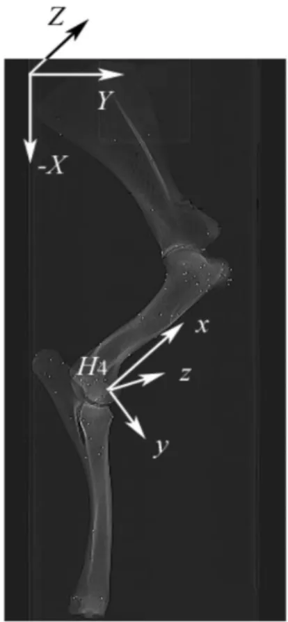
9. CT scan of the lateral side of the scapula, humerus, radius, and ulna. Metallic markers are embedded to represent muscle origins and insertions, contact points, and additional key locations. The top axis (X, Y, Z) represents the global coordinate, while (x, y, z) represents the local humeral system. The x axis was defined as distal to proximal, the y-axis was caudal to cranial, and the z-axis was lateral to medial (Pollock et al., 2008a) ………… 26
10. Example of a typical in vitro materials testing machine containing a lateral view of a left equine forelimb. This set up was used in Pollock’s (2008b) study where a mechanical model (Musculoskeletal Model II) was used to validate the mathematical model (Musculoskeletal Model I) by comparing
x
LIST OF FIGURES
Figure Page 11. Free body diagrams of a left humerus with muscle and contact forces
applied for all load cases from the (a) lateral, (b) medial, and (c) caudal views. Arrows along each axis indicate positive directions
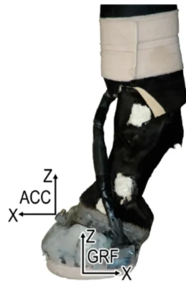
(Ferullo, 2007) ………... 30-31 12. A dynamometric horseshoe fixed to the solar surface of the hoof recorded
ground reaction forces (GRF), while a tri-axial piezoelectric accelerometer fixed to the dorsal part of the hoof wall of the left forelimb recorded
accelerations (ACC). The coordinate arrows represent the positive Z and X axes of each coordinate system, and were fixed to the solar surface of the hoof (Setterbo et al., 2007) ……….. 39 13. Dirt, turf, and synthetic vertical ground reaction forces (Z-force) during
trot. Trot was defined as having a mean velocity of roughly 5 m/s
(Setterbo et al., 2007) ………... 41 14. Percent change in porosity recorded every 10 days. The blue lines indicate
the criteria for equilibrium, which is a less than 5% change in remodeling
parameters (Ferullo, 2007) ………... 49
15. Percent change in damage recorded every 10 days. The blue lines indicate the criteria for equilibrium, which is a less than 5% change in remodeling
parameters (Ferullo, 2007) ………... 50
16. Percent change in BMU activation frequency recorded every 10 days. The blue lines indicate the criteria for equilibrium, which is a less than 5% change in remodeling parameters (Ferullo, 2007) ………... 50
17-18. BMU activation frequency (BMUs/mm2/day) recorded every 10 days for 350 days at the stress fracture site and caudal diaphysis during the Baseline Layup and Long Layup training programs (Ferullo, 2007). Model comparison between Ferullo’s (2007) results (top) and current model results (bottom) validate the current model ………... 54 19-20. Porosity (%) recorded every 10 days for 350 days at the stress fracture site and
caudal diaphysis during the Baseline Layup and Long Layup training programs (Ferullo, 2007). Model comparison between Ferullo’s (2007) results (top) and current model results (bottom) validate the current model ……….. 55
21-22. Percent increase in damage over the equilibrium value (stress fracture site = 0.0299mm/mm2, caudal diaphysis = 0.1003 mm/mm2) recorded every 10 days for 350 days at the stress fracture site and caudal diaphysis during the Baseline Layup and Long Layup training programs (Ferullo, 2007). Model comparison between Ferullo’s (2007) results (top) and current model results (bottom)
xi
LIST OF FIGURES
Figure Page 23. Damage (mm/mm2) recorded every 10 days for 160 days of training at the
stress fracture site and caudal diaphysis during Race Program 1 ………... 58
24. Damage (mm/mm2) recorded every 10 days for 160 days of training at the stress fracture site and caudal diaphysis during Race Program 2 ……… 59 25. BMU activation frequency (BMUs/mm2/day) recorded on the 90th, 120th, and
150th days of training at the stress fracture site and caudal diaphysis during Race Program 1 and 2 ……….. 59 26. Porosity (%) recorded on the 90th, 120th, and 150th days of training at the stress
fracture site and caudal diaphysis during Race Program 1 and 2 ……… 60
27. Damage (mm/mm2) recorded on the 90th, 120th, and 150th days of training at the stress fracture site during Race Program 1 and 2 ………... 60
28. Damage (mm/mm2) recorded on the 90th, 120th, and 150th days of training at the caudal diaphysis during Race Program 1 and 2 ………. 61 29. Percent increase in damage over the equilibrium value (stress fracture site =
0.0299 mm/mm2)recorded every 10 days for 350 days at the stress fracture site during the Baseline Layup training program for dirt (Ferullo, 2007), turf, and synthetic track surfaces ……… 62 30. Percent increase in damage over the equilibrium value (caudal diaphysis =
0.1003 mm/mm2) recorded every 10 days for 350 days at the caudal diaphysis during the Baseline Layup training program for dirt (Ferullo, 2007), turf, and synthetic track surfaces ……… 62
31. Percent increase in damage over the equilibrium value (stress fracture site = 0.0299 mm/mm2) recorded every 10 days for 350 days at the stress fracture site during the Long Layup training program for dirt (Ferullo, 2007), turf, and
synthetic track surfaces ……… 63
32. Percent increase in damage over the equilibrium value (caudal diaphysis = 0.1003 mm/mm2) recorded every 10 days for 350 days at the caudal diaphysis during the Long Layup training program for dirt (Ferullo, 2007), turf, and
synthetic track surfaces ……… 63
33. Damage (mm/mm2) recorded every 10 days for 160 days of training at the stress fracture site and caudal diaphysis during Race Program 1 for dirt, turf, and synthetic track surfaces ………. 64
xii
LIST OF FIGURES
Figure Page 35. BMU activation frequency (BMUs/mm2/day) recorded every 10 days for
350 days at the stress fracture site during the Baseline Layup training
program for dirt (Ferullo, 2007), turf and synthetic track surfaces ………….… 66 36. BMU activation frequency (BMUs/mm2/day) recorded every 10 days for
350 days at the caudal diaphysis during the Baseline Layup training
program for dirt (Ferullo, 2007), turf, and synthetic track surfaces ……… 66 37. Porosity (%) recorded every 10 days for 350 days at the stress fracture site
during the Baseline Layup training program for dirt (Ferullo, 2007), turf, and synthetic track surfaces ……… 67
38. Porosity (%) recorded every 10 days for 350 days at the caudal diaphysis during the Baseline Layup training program for dirt (Ferullo, 2007), turf, and synthetic track surfaces ……… 67
39. BMU activation frequency (BMUs/mm2/day) recorded every 10 days for 350 days at the stress fracture site during the Long Layup training program for dirt (Ferullo, 2007), turf and synthetic track surfaces ……… 69
40. BMU activation frequency (BMUs/mm2/day) recorded every 10 days for 350 days at the caudal diaphysis during the Long Layup training program for dirt (Ferullo, 2007), turf and synthetic track surfaces ……… 69
41. Porosity (%) recorded every 10 days for 350 days at the stress fracture site during the Long Layup training program for dirt (Ferullo, 2007), turf, and
synthetic track surfaces ……… 70
42. Porosity (%) recorded every 10 days for 350 days at the caudal diaphysis during the Long Layup training program for dirt (Ferullo, 2007), turf, and
synthetic track surfaces ……… 70 43. BMU Activation Frequency (BMUs/mm2/day) recorded every 10 days for
160 days at the stress fracture site and caudal diaphysis during Race Program 1 for dirt, turf, and synthetic track surfaces ……… 72 44. BMU Activation Frequency (BMUs/mm2/day) recorded every 10 days for
160 days at the stress fracture site and caudal diaphysis during Race Program 2 for dirt, turf, and synthetic track surfaces ……… 72 45. Porosity (%) recorded every 10 days for 160 days at the stress fracture site
xiii
LIST OF FIGURES
Figure Page 46. Porosity (%) recorded every 10 days for 160 days at the stress fracture site
and caudal diaphysis during Race Program 2 for dirt, turf, and synthetic
track surfaces ………... 73 47-48. A fitted line plot observing the correlation between step (4 steps in a day) and
percent increase in damage at the stress fracture site for Race Program 1 (top) and Race Program 2 (bottom) with an R-Squared value (Coefficient of
I. Introduction
Thoroughbred Racehorse Injuries
Thoroughbred race horses, which are between two and three years of age,
commonly experience humeral stress fractures at a characteristic location making them a
useful model in this study. Thoroughbred racehorses can experience multiples injuries
during intense periods of training, such as bucked shins or humeral stress fractures, where
70% of young Thoroughbred racehorses develop bucked shins as a result of repetitive
loading injury in their third metacarpal bone (MCIII) (Nunamaker, 2002b). When a
horse has a musculoskeletal injury, it is important to have a period of layup or rest to
allow the damaged area to heal. If the horse becomes injured to the point where they are
no longer able to recover, then they are highly susceptible to fracture, which can cost the
owner a substantial investment, where the median sale price of a Thoroughbred between
the age of 1 and 2 years is $40,000 (Burr and Milgrom, 2001). The frequency of equine
injury coupled with a high-priced investment makes it practical to implement and
investigate new training programs, which not only prevent equine musculoskeletal injury,
but allows equine athletes to stay physically competitive.
Thoroughbred racehorses between 2 to 3 years of age are more at risk to
musculoskeletal injury compared to older Thoroughbreds since younger Thoroughbred’s
bones are still maturing, are more porous, and have yet to adapt to the racing environment
(Boston and Nunamaker, 2000). Mature horses have a large bone radius when compared
to younger horses, which allows for lower stress at similar forces due to a greater cross
sectional area of bone. Also, it is more likely stress fracture can occur if the horse is
stiff muscles at a high frequency (Hernandez et al., 2001). Previous studies have shown
that incorporating a walking exercise into the horse’s training schedule reduces the
chance of having bucked shins (Mattila et al., 2007). In the current study, four separate
training programs were investigated, which include layup programs Baseline Layup and
Long Layup, and two new race programs.
Along with training regimes, additional environmental influences can play a role
in the development of equine musculoskeletal injury. Track surface material type, such
as dirt, turf, and synthetic, contribute to different effects on ground reaction forces and
hoof accelerations during trot and canter (Setterbo et al., 2007). Compared to dirt, turf
proved to be associated with lower risk for injury in one study (Mohammed et al., 1991),
while another showed the complete opposite (Hernandez et al., 2001). There are frequent
contradictions and inconsistencies in previous literature on correlation between risks of
equine musculoskeletal injury and track surface type. Although it has been statistically
proven that turf, synthetic, and dirt track surfaces contribute to different hoof ground
reaction forces and accelerations during gallop (Setterbo et al., 2007), many believe the
softer tracks are more advantageous and physically safer for equine races since dirt
surfaces have been replaced with synthetic materials at several different race courses over
the last 3 years (Setterbo et al., 2007). In the current study, we employ previously
calculated hoof ground reaction forces from dirt, turf, and synthetic surfaces (Setterbo et
al., 2007) to investigate their effects in a computational model on bone remodeling in a
The Characteristics, Function, and Biology of Bone
Bone Composition
Bone is composed of 25% water, 32% organic matrix, and 43% apatite mineral,
which includes collagen, hydroxyapatite, and small portions of proteoglycans and
noncollagenous proteins (Martin et al., 1998). Collagen is a structural protein organized
to create strong fibers, which provide high tensile strength and flexibility to bone, where
the most common type of collagen found in bone is type I. Hydroxyapatite
[Ca10(PO4)6(OH)2] crystals account for the majority of bone’s dry weight and are key for
providing bone with compressive strength and rigidity. Proteoglycans participate in
modulating collagen fibril assembly (Martin et al., 1998). While bone is composed of all
these components, its material properties can vary depending on apparent density and
porosity (Nunamaker, 2002a).
Bone Function
The primary functions of bone include providing a foundation for other organs to
adhere to, protecting organs from exterior trauma, and transmitting forces from one area
of the body to a desired location. Bone is designed to bear the weight of loads with
minimal deformation and has a high strength to weight ratio. Bone is known to model
based on the load it receives by changing its morphology to reduce stresses (Boston and
Nunamaker, 2000). Bone changes its geometry to efficiently withstand future loads,
which is known as Wolff’s Law where bone becomes aligned in principal stress
directions. Marrow is contained within the medullary canal of bone and is a tissue
generating new blood cells (Martin et al., 1998). Bone vasculature is maintained through
the medullary canal and periosteal blood supply. Circulation in bone is centripetal, where
the afferent blood supply consists of arteries and arterioles and the efferent blood supply
is composed of veins and veinules (Nunamaker, 2002a). While bone is perceived by
most as a stagnant inert structure, it is dynamic and continuously changing its
composition and microscopic architecture due to mechanical stimuli and other
environmental factors.
Bone Tissue Types
There are two types of bone tissue called trabecular and cortical bone. Cortical
bone or sometimes referred to as compact bone, is dense, has a porosity (void
volume/total volume) of 5%-10%, and is mainly found in shafts of long bones and forms
a cortex around vertebral bodies and other spongy bones (Martin et al., 1998). Within
cortical bone, there are porous spaces composed of Haversian canals, Volkmann’s canals,
and resorption cavities. Haversian canals are aligned along the length of the bone and
contain capillaries, nerves, and are about 50 µm in diameter (Martin et al., 1998).
Volkmann’s canals also contain blood vessels along with nerves and are transverse canals
connecting Haversian canals to each other and to the outside surface of bones (Martin et
al., 1998). Resorption cavities are about 200 µm in diameter and are temporary pits
created by bone cells which remove bone known as osteoclasts. Figure 1 shows typical
features of a long bone.
Figure 1. Sketch of typical long bone features (Martin et al., 1998).
Trabecular or cancellous or spongy bone contains interconnected pores filled with
bone marrow and has a porosity of 75%-95%. Trabecular bone is found in the vertebrae,
flat bones, and ends of long bones. The bone matrix of trabecular bone normally resides
on the endosteum of long bone and forms struts called trabeculae, which are
approximately 200 µm thick. Trabeculae can either be randomly organized or form
orthogonal arrays. Both cortical and trabecular bone contain two types of bone tissue
known as lamellar bone and woven bone (Martin et al., 1998). Lamellar bone is highly
organized and slowly formed with an anisotropic matrix, which means its material
properties change depending on direction. The anisotropic matrix consists of highly
organized parallel layers or lamellae of mineral crystals and collagen fibers. Woven bone
randomly arranged (Martin et al., 1998). Woven bone is primarily used to temporarily
bridge stress fractures to alleviate stress.
Cortical bone tissue contains two categories; primary and secondary bone.
Primary bone lays down new bone on an existing surface during growth, such as the
periosteal surface (Martin et al., 1998). Within primary bone, there are two general types
called circumferential lamellar bone and plexiform bone. Circumferential lamellar bone
contains a matrix of lamellae parallel to the surface of the bone. When blood vessels
become incorporated into new periosteal bone, they become surrounded by circular
lamellae, which form primary osteons with a primary Haversian canal at the center
(Martin et al., 1998). Plexiform bone has a high rate of formation and is a mixture of
woven bone (trabeculae) and lamellar bone. Within plexiform bone are rectilinear
vascular spaces, which give an appearance of a “brick wall.” Plexiform bone is found in
larger animals such as cows and horses. It may also aide in fatigue resistance for
racehorses (Stover et al., 1992). Secondary bone results in the removal of existing bone
and replacement with healthy, lamellar bone by a process known as remodeling in which
teams of bone cells work together to replace old retired bone with new healthy bone.
Secondary bone contains cylindrical systems of Haversian canals and secondary osteons
(formed through remodeling). For human adults, compact bone is entirely composed of
secondary bone and trabecular bone is also mostly secondary bone, but trabecular bone
rarely produces osteons since they cannot fit inside individual trabeculae (Martin et al.,
Bone Cells
Bone is a dynamic structure in which remodeling takes place to remove old bone
and replace it with new bone, which is initiated by: microdamage, chemical factors,
fracture, bone age, and mechanical environment. There are a total of four different types
of bone cells known as osteoblasts, osteoclasts, osteocytes, and bone lining cells. The
bone cells responsible for removing and replacing bone are known as osteoclasts and
osteoblasts, respectively. Osteoclasts tunnel through bone and remove it, while
osteoblasts follow, laying down new healthy bone. Collectively, these teams of
osteoblasts and osteoclasts are known as basic multicellular units or BMUs. Osteocytes
are former osteoblasts which became embedded in the bone matrix by being engulfed by
faster, more active osteoblasts. Osteocytes reside in cavities known as lacunae, where
they communicate with osteoblasts with processes passing through tunnels called
canaliculi (Martin et al., 1998). Bone lining cells are also quiescent osteoblasts, which
reside flattened on the surfaces of bone and aide in communication with osteocytes by
using gap-junctioned processes (Martin et al., 1998). Bone lining cells contain receptors
for parathyroid hormone, estrogen, and other chemical messengers. Both osteocytes and
bone lining cells are responsible for the transfer of mineral into and out of bone. The
combination of all four bone cells allows the microstructure of bone to repair,
communicate with other cells, and transfer necessary nutrients.
Osteoblasts differentiate from mesenchymal stem cells, which derive from the
stromal tissue of bone marrow. Complete differentiation of mesenchymal stem cells can
take 2-3 days (Martin et al., 1998) and is initiated through mechanical stress to bone
contains collagen and noncollagenous proteins, proteoglycans, and water (Martin et al.,
1998). Osteoid is laid down by osteoblasts at an apposition rate of approximately 1
µm/day. Unlike osteoblasts which are mononuclear, osteoclasts are multinuclear,
produced by the fusion of monocytes originating from the hemopoeitic portion of bone
marrow (Martin et al., 1998). When osteoclasts break down and resorb bone, it occurs
along the ruffled border of the cell, which is sealed to the bone surface. The resorption
rate of osteoclasts is approximately 10 µm/day and is accomplished through the
production of acids and enzymes, which demineralize adjacent bone and dissolve
collagen, respectively.
Modeling and Remodeling
This study is aimed at the process of remodeling in which teams of osteoblasts
and osteoclasts work together to remove and replace bone at a specific location.
Modeling is where bone is removed in certain areas (osteoclastic activity) and added to
others (osteoblastic activity), so osteoblasts and osteoclasts are working independently.
When compared to remodeling, modeling is greatly reduced after skeletal maturity.
Modeling also results in the change of bone size and shape, but remodeling normally
does not affect size or shape. Both of these features of bone are necessary for the proper
development and renovation of the skeleton.
Modeling allows the geometry and size of the skeleton to develop correctly and
can be resorptive or formative while a child is developing. It allows bone to customize
itself based on loads it receives, which give it optimal material and mechanical properties
microdamage in which osteoclasts work to remove old bone and osteoblasts follow
replacing it with new bone. It has also been hypothesized that remodeling mechanically
“fine tunes” the skeleton to increase mechanical efficiency (Martin et al., 1998). BMUs
(Basic Multicellular Units) are a collective team of several hundred osteoblasts and
approximately 10 osteoclasts. During a life of a BMU it undergoes three main stages:
activation, resorption, and formation. Activation is initiated through a chemical or
mechanical signal causing osteoclasts to form. Osteoclasts resorb a volume of bone in
the form of a trench for bone surfaces and create a tunnel (200 µm in diameter) in
compact bone, moving at approximately 40 µm/day. When osteoclastic activity begins to
slow, osteoblasts start differentiating from mesenchymal stem cells and initiate bone
tissue formation over the removed tissue (Martin et al., 1998).
Secondary osteons are created by BMU tunnels in cortical bone. BMUs are
responsible for replacing approximately 5% of compact bone each year in adult humans.
In trabecular bone, BMUs work at the surface by digging and refilling trenches. The
average human adult BMU replaces approximately 25% of trabecular bone per year
(Martin et al., 1998). Compared to human bone, equine bone has more bone volume,
which indicates a higher probability of damage, so the frequency of remodeling is greater
Figure 2. Illustration of the creation of a secondary osteon through the resorption of osteoclasts followed by osteoblasts, which are forming new bone to establish a newly remodeled haversian system (Nunamaker, 2002a).
There are six separate phases to bone remodeling: activation, resorption, reversal,
formation, mineralization, and quiescence. During activation (3 days), osteoclasts are
created and recruited to the site of interest. For the resorption period, osteoclasts begin
to break down and resorb bone (Martin et al., 1998). During the reversal period, there is
a transition from osteoclast to osteoblast activity, which takes several days and a visible
line (cement line) is formed where the osteoclasts cease activity. The porosity of bone
temporarily increases after the resorption period, thus decreasing the elastic modulus.
The resorption and reversal periods combined take about 30 days. After the reversal
period, the formation period begins (this phase in adult humans lasts about 3 months) and
osteoblasts fill in new bone, starting at the periphery of the tunnel created by the
osteoclasts (Martin et al., 1998) (Figure 2). Osteoblasts do not completely refill the
which create secondary osteons (Figure 3). After formation, the bone site is mineralized
and goes into quiescence, where there is a period of inactivity.
Figure 3. Microradiograph of remodeling in horse bone within the cortex. The larger black areas represent resorption cavities, while the grey oval shaped areas represent new-less calcified bone making up secondary osteons (Nunamaker, 2002a).
Material and Mechanical Properties
Bone is a viscoelastic material, meaning it is both viscous (resistant to flow) and
elastic (can withstand permanent deformation). Collagen gives bone its elastic properties
in tension, while hydroxyapatite supplies a high compressive elastic modulus. The elastic
modulus for equine cortical bone is approximately 18-20 GPa (Nunamaker, 2002a),
which is similar to human cortical bone with an average of 17.9 GPa (Reilly et al., 1974)
in the longitudinal direction. It is also anisotropic, meaning its material properties
depend on orientation. Bone is strongest in compression and weakest in tension, but its
strength depends on the direction of loading. Longitudinally bone is stronger compared
the longitudinal direction of 205 MPa and 131 Mpa in the transverse direction, while the
ultimate tensile strength is 135 MPa in the longitudinal direction and 53 MPa in the
transverse direction (Table 1).
Cortical bone mechanical properties of the cortex are the result of the following
osteon activities: replacing highly mineralized bone matrix with less calcified material,
increasing cortical porosity, altering collagen fiber orientation, and incorporating cement
line interfaces, which have unique mechanical properties. Collage fiber orientation can
affect bone strength, stiffness, density, porosity, and mineralization (Martin et al., 1998).
Porosity can affect bone density, stiffness, and be an indicator for a potential stress
fracture. Porosity, mineralization, density, histological architecture, collagen fiber
organization, fatigue damage, and rate of deformation are all factors affecting the
material properties of cortical bone (Martin et al., 1998).
Table 1. Anisotropic data from a bovine and human bone (Reilly et al., 1974; Reilly and Burstein, 1975).
Tension Compression
Elastic Modulus, Gpa Longitudinal Transverse Longitudinal Transverse
Human
Haversian 17.9 10.1 18.2 11.7
Bovine
Haversian 23.1 10.4 22.3 10.1
Primary 26.5 11 N/A N/A
Tension Compression
Ultimate Stress, Mpa Longitudinal Transverse Longitudinal Transverse
Human
Haversian 135 53 205 131
Bovine
Haversian 150 49 272 146
Stress Fractures
Stress fractures can range from small microcracks to complete fractures through
the entire bone and are induced by repetitive mechanical loading of the bone. They are
commonly seen in military recruits, long distance runners, and race horses. Stress
fractures and their development can be predicted by looking at the damage, BMU
activation frequency, porosity, strain, modulus and stress at a specific area on a
Thoroughbred’s humerus. Cyclic stresses in bone can lead to microdamage, which
initiates remodeling, where osteoclasts began to remove damaged bone, which
temporarily increases porosity, thus reducing the elastic modulus. This is the primary
method in which bone addresses stress fractures, but the strain of the bone increases and
becomes susceptible to fracture (O'Sullivan and Lumsden, 2003). For more unstable
stress fractures, osteoblasts will bridge the stress fracture gap and lay down woven bone
forming a callus. Calluses form to adapt to stress fractures allowing for increased loading
and to enlarge bone area, which decreases strain (Johnson et al., 1994). The risk for
stress fracture increases when an exercise suddenly becomes more rigorous, such as
runners increasing mileage or running frequency. This same theory can be applied to a
racing horse, so within this study’s exercise simulation; distance should be increased over
a longer period of time.
In a previous study, humeral stress fractures were seen more often in 3-year-old
Thoroughbreds, when compared to tibial stress fractures, which were predominately seen
in 2-year-old Thoroughbreds. Additionally, humeral stress fractures were more
commonly seen in extensively raced Thoroughbreds, while lightly raced horses were
fractures in young human athletes between 19 and 25 years of age represent
approximately 70% of all reported stress fractures in runners (Hazelwood and Castillo,
2007). In the current study, there are two sites of interest on the humerus: a region
known to be consistently associated with stress fractures known as the caudoproximal
stress fracture site and a control location for comparison called the caudal diaphysis
(Figure 4). The stress fracture site and caudal diaphysis were chosen since they provide
sufficient mechanical testing data from a previous study (Entwistle et al., 2009). This
study explored the differences between materials properties in a healthy bone and
callused bone (Entwistle et al., 2009). Stress fractures are ideal to study due to their
predictable locations and frequency among athletes.
Figure 4. (a) Lateromedial radiographic projection of one half of the Thoroughbred right humerus cut along the sagittal plane. The red box indicates the location of the stress fracture site at the caudoproximal region. The green box displays the caudal aspect of the diaphysis. (b) The cranciocaudal radiographic projection of the complete right humerus (Ferullo, 2007).
The Entwistle et al. (2009) study conducted mechanical testing on equine humeri,
and without, stress fracture. Cortical beams and cores were harvested from the stress
fracture site and a site distant from the affected region (caudal diaphysis), respectively.
The humeri were classified as having an absence of stress fracture (stage 0) or having a
presence of stress fracture with a callus maturity from stages 1-3 (Entwistle et al., 2009).
These samples were then tested to failure at an apparent strain rate of 0.01sec-1 obtaining
material properties from each section. It was found that cortical beam specimens
underwent a reduction in material properties, such as a decrease in modulus as the callus
staged progressed. At the caudal diaphysis, material properties were initially reduced,
but then recovered to control levels as the stage of the callus progressed (Entwistle et al.,
2009).
The affected cortical beam specimens produced median longitudinal moduli of
15.5 GPa, 17.3 Gpa, and 9.3 GPa for callus stages 1, 2, and 3, respectively, while the
median for the control specimens was 17.4 GPa. The median elastic moduli taken from
the cores at the caudal diaphysis were 12.8 GPa, 14.0 GPa, and 14.8 GPa for callus stages
1, 2, and 3, respectively, while the median modulus was 14.7 GPa for the unaffected
specimens (Entwistle et al., 2009). Two different types of specimens (beams and cores)
were used for mechanical testing at the stress fracture site and caudal diaphysis, which
explains the difference in modulus between the two. Additionally, 18 Thoroughbred
racehorses of ages 2-4 were used (Entwistle et al., 2009), which give a range of moduli
since it is dependent on equine age and training stage of the horse. In the current model,
at the begging of training for each program, the modulus for the stress fracture site and
Finite Element Analysis
Finite element modeling is a useful tool for analyzing stresses and strains in bone
at the macro scale. It is a numerical system where stresses, strains, and other mechanical
properties are computationally solved within a solid volume, such as a humerus. The
volume of the model is divided up into elements (mesh), which have a set of mechanical
and materials properties (Martin et al., 1998). Specific material properties such as
density, porosity, and elastic modulus can be defined within each element. Boundary
conditions, which either supply loads or provide restrictions to the model, can also be
applied. The number of elements used will determine the resolution of the mesh and the
entire model; with an increasing number of elements making the model more accurate.
After boundary conditions, material properties, orientation, and geometry are defined,
computational modeling is used to solve a system of equations, which can determine the
model’s deformation and stress contours along with other results.
Finite element modeling and simulations have become an alternative to traditional
laboratory tests with the increasingly availability of powerful computers along with more
affordable prices (Ross, 2005). Traditional laboratory tests are time consuming, costly,
and require more material. It is also difficult to use experimental devices, such as strain
gauges, within a complex geometry of bone, like the temporomandibular joint (Figure 5)
in humans (Beek et al., 2000). Finite element modeling has the ability to mesh and
observe strain contours of bone containing highly irregular geometries. Finite element
modeling is an important tool in orthopedics due to irregular bone shapes and varying
investigating stress fractures produced from: racing, impact from various track surfaces,
and training regimes.
Figure 5. Three-dimensional finite element lateral display of the right human temporomandibular joint (Beek et al., 1999).
To model the mechanical behavior of a Thoroughbred racing horse humerus, this
study used ABAQUS (SIMULIA, Providence, RI), a finite element program where
loading and boundary conditions can be applied to a mesh based on the bone’s geometry.
For the 3D finite element model of the horse humerus, the loading conditions are
represented by nine muscle forces and two contact forces, while the distal end of the
humerus is fixed as a boundary condition. The muscle force and contact force values
placed in FEA model were found from a previous study, which used a mathematical
model and a physical testing system consisting of a test fixture, weights, and strain
gauges (Pollock et al., 2008a; Pollock et al., 2008b). Also within the finite element
model, there are four different loading conditions representing standing, fore-stance,
four steps. There are 1400 steps in each simulation for the Baseline Layup and Long
Layup training programs, which yields 350 days of training per simulation. The race
programs have a total of 672 steps, which is 168 days of training and racing. At any of
these steps the material behavior of the humerus can be observed by looking at stress
contours, strain, and deformation within ABAQUS (SIMULIA, Providence, RI), but in
this study the state variables of interest are bone porosity, BMU activation frequency, and
damage, which are tracked with a remodeling algorithm at the two humeral sites of
interest.
Bone Remodeling Algorithm
The remodeling algorithm developed by Hazelwood et al. (2001) is employed into
the finite element model and simulates changes in bone’s elastic modulus and porosity
resulting from damage and the mechanical environment. This algorithm was initially
designed to be incorporated into a finite element model representing a small bone volume
or an entire bone (Ferullo, 2007). This simulation uses 8 state variables, which are
updated throughout each step of the model and include: elastic modulus, porosity,
number of resorbing and refilling BMUs, BMU activation frequency, normalized specific
area, damage, strain, and mechanical stimulus. Tables 6 and 7 display state variables and
constants with their respective values. At every step during the training regime, bone
elastic modulus and porosity are updated as a result of damage formation, damage
removal, or disuse. The schematic below (Figure 6) displays the representation of the
bone remodeling algorithm by Hazelwood et al. (2001) and features two separate
damage removal, while the left loop increasing the rate of remodeling, which increases
porosity, strain, and damage formation (Hazelwood et al., 2001).
Figure 6. Schematic of bone remodeling algorithm. This system contains two feedback loops, where the right side results in damage removal and the left side results in increased porosity, strain, and damage formation (Hazelwood et al., 2001).
The bone remodeling algorithm was incorporated into the finite element model in
the current study to investigate stress fractures and bone material property changes in the
equine humerus as a result of training regimes, track surface properties, muscle and joint
contact loads. The current algorithm was implemented in FORTRAN and designates the
activities to which the FEA humerus will undergo by assigning the duration of slow and
fast gallops to each step of the gait cycle. The program where the bone remodeling
algorithm resides also determines the distance the horse will run depending on the day of
the training program. A separate case in the simulation assigns the days a horse will
perform a layup, where only the standing case is applied, so the slow and fast gallop
variables are set to zero. Every Thoroughbred training program in the current study used
Hazelwood et al.’s (2001) bone remodeling algorithm was used in this study due
to its successful contribution to multiple previous studies with different applications in
which it is employed with an FEA model to simulate changes in bone material properties.
One study observed the effects of marathon training on bone density, remodeling, and
microdamage in the human femur. Similar to horse training programs in the current
study, different marathon training programs were used for comparison to observe
differences in bone damage, density, and activation frequency (Hazelwood and Castillo,
2007). Another study used the same bone remodeling algorithm to simulate and compare
stress shielding effects in the femoral head due to resurfacing of the hip and a total hip
anthroplasty (Deuel, 2007). This study was able to determine bone loss due to stress
shielding from different modes of hip surgery. Hazelwood et al.’s (2001) bone
remodeling algorithm will continuously be updated to create additional simulations and
will be incorporated into further bone remodeling computational studies.
Layup Training Programs and Race Programs
Ferullo’s (2007) study had four different programs lasting 350 days, where each
had different periods of layup representing healing periods following injury to the horse.
The objective of that study was to compare the mechanism of bone remodeling between
the four layup programs. The layup training programs included: Baseline Layup, Long
Layup, Short Layup, and Split-Fast Gallop training programs. Layup for the Baseline
Layup, Long Layup, and Short Layup training programs lasted 8 weeks, 16 weeks, and 5
weeks respectively. The Split-Fast Gallop program had a layup period exactly the same
week, where the horse ran a fast gallop twice a week at half distance. The Baseline
Layup and Long Layup programs were used from Ferullo’s (2007) study to validate
simulation files in the current study.
It was found from Ferullo’s (2007) study that training programs with a period of
longer layup displayed lower values for damage when compared to programs with shorter
periods of layup. Bone is given time to remodel and remove damage during longer
periods of layup. Training programs with shorter periods of layup apply more loading
cycles and contribute to increased microdamage at the stress fracture site. However,
training programs with longer periods of layup increase the porosity of bone making it
more susceptible to fracture at the return of training. Training programs without a period
of layup would have a tighter control on the porosity and elastic modulus at the stress
fracture site and caudal diaphysis within the humerus.
Two new programs, known as the race programs, were implemented in the current
investigation to study bone remodeling during a training regime without a period of
layup. These programs did not incorporate a period of layup, which would not allow
bone cells to increase porosity. When porosity in the humerus is increased, the bone’s
susceptibility to stress fracture increases. It is common for stress fractures to occur
during the sudden onset of increased microdamage, which is commonly seen during
training within 3 weeks after layup (Carrier et al., 1998). Even though microdamage
would accumulate for a program without a period of layup, the higher elastic modulus
coupled with workout loads might be able to inhibit a catastrophic stress fracture when
Goals and Hypotheses
The three main goals in the current study included: implementing and validating a
working Thoroughbred humerus model in ABAQUS (SIMULIA, Providence, RI) using
previously created ABAQUS (SIMULIA, Providence, RI) input files and FORTRAN
script files by Ferullo (2007), creating two entirely new training programs (race
programs) and comparing them between each other, and lastly incorporating turf and
synthetic track surface properties into all training programs by scaling down muscle and
contact forces. Data was gathered at two sites of interest (Figure 4) on the Thoroughbred
racing humerus: the stress fracture and caudal diaphysis sites. The training programs
observed underwent different periods of layup, initial training, race programs, and length
of exercise.
This study encompassed three hypotheses. The first hypothesis was the FEA
model of the current study will produce the same results for the Baseline Layup and Long
Layup training programs as those seen in the previously validated model of Ferullo
(2007). The second hypothesis was Race Program 1 will accumulate more microdamage
when compared to Race Program 2 since Race Program 1 immediately undergoes a race
on the first week of race training. Race Program 2 has a bye during the same week with a
day of slow gallop instead of a race, which produces less damage allowing the horse to
recover throughout training in comparison to Race Program 1. The third hypothesis was
turf and synthetic track surfaces will contribute smaller loads when compared to dirt track
surfaces causing less bone damage for all training programs at the stress fracture site and
caudal diaphysis. Less bone damage implies a lower damage removal rate, lower BMU
Additionally, smaller loads can lead to disuse, which increases BMU activation
frequency and increases porosity by removing unnecessary bone (bone remodels in
response to the load it receives).
II. Methods
Development of Finite Element Model
A CT scan of a healthy humerus from a 6-year-old Thoroughbred was placed into
Mimics (Materialise, Ann Arbor, MI) to create a 3-dimensional model of the outer
cortical and articular surfaces of an equine humerus. The CT scan contained 370 images
of 2mm thick sections with a 1mm overlap (Ferullo, 2007). The surface of the scanned in
solid model was automatically meshed using triangular elements in Mimics. Element
reduction tools were used to reduce the total number of elements and increase element
quality. A surface mesh of the humerus of 5154 total elements was then exported to
Patran (MSC Software, Santa Ana, CA) (Ferullo, 2007).
A solid tetrahedral mesh was created using the surface mesh generated in Mimics.
The 10-noded tetrahedral elements had 4 integration points (Ferullo, 2007). A tetrahedral
mesh was applied to the solid model due to short processing time and low number of
degrees of freedom required for convergence (Viceconti et al., 1998). A 1334N point
load (Pollock et al., 2008a) was applied at approximately the shoulder joint contact force
location of a standing horse on the mesh, and a static analysis was executed to find
displacement at a standard location and to find the number of nodes required for results to
converge (Ferullo, 2007) (Figure 7). The ABAQUS (SIMULIA, Providence, RI) finite
Figure 7. Demonstration of model convergence with maximum displacement (mm) of tetrahedral meshes depending on number of nodes (Ferullo, 2007).
A 13,596 element solid tetrahedral mesh with 20,569 nodes was selected as the
final finite element model. Within this model, 96 of the most distal CT slices of the
humerus were removed in Patran (MSC Software, Santa Ana, CA) while fixating the
distal surface. The distal end of the humerus was fixated since it was determined that
forces on the distal portion of the humerus do not affect proximal stresses in the areas of
interest (Ferullo, 2007). This model was chosen due to a low run time, averaging 48
seconds/step for Ferullo’s (2007) runtime and 10 seconds/step for the current study’s
runtime since the current study had a faster processor. Additionally, the current model
was chosen due to its normal humeral geometry (Figure 8), rather than incorporating a
Figure 8. From left to right: medial, cranial, and caudal views of the mesh of the humerus displaying the regions of interest including the Stress Fracture Site (a) and the Caudal Diaphysis (b). The Cranial Aspect of the Diaphysis (c) was not an area of interest and was only used to validate the results from the region of the Caudal Diaphysis (b) (Ferullo, 2007).
Contact and Muscle Forces
The current model represents a racing Thoroughbred humerus which takes into
account joint reaction forces, muscle forces, and four separate loading conditions
representing fore-stance, mid-stance, aft-stance, and standing. Contact and muscle forces
magnitudes and direction vary depending on position and speed during the gait cycle.
A right cadaveric forelimb from a euthanized 4-year-old Thoroughbred gelding
was used in a previous study to determine muscle force, origin, insertion, and direction
(Pollock et al., 2008a). At each muscle origin and insertion, metallic markers were
embedded to determine location. Following this, a CT scan was performed while the
coordinates of each muscle’s origin and insertion locations relative to one another
(Beaupre et al., 1990a; Beaupre et al., 1990b). The humeral coordinate system origin
was placed between the distal condyles on the humerus (Figure 9). EMG data during the
stance phase of walking from equine (Korsgaard, 1982) and canine (Tokuriki, 1973)
forelimb muscles was used to determine whether muscles were activated while the horse
was walking.
Figure 9. CT scan of the lateral side of the scapula, humerus, radius, and ulna. Metallic markers are embedded to represent muscle origins and insertions, contact points, and additional key locations. The top axis (X, Y, Z) represents the global coordinate, while (x, y, z) represents the local humeral system. The x-axis was defined as distal to proximal, the y-axis was caudal to cranial, and the z-axis was lateral to medial (Pollock et al., 2008a).
The values of humeral muscle forces were predicted using optimization
techniques and each muscle’s maximum force during voluntary contraction (MVC) was
tension of 15 N/cm2 (Powell et al., 1984). PCSA values were estimated by determining
muscle volume and length during gross dissection (Pollock et al., 2008a). The biceps
brachii contact force was found using a materials testing machine in vitro (Figure 10).
The scapula contact force was determined after the forces of the muscles that crossed the
shoulder joint in the model were determined (Pollock et al., 2008a). Tables 2 and 3 show
activation levels of selected muscles attached to the humerus.
Figure 10. Example of a typical in vitro materials testing machine containing a lateral view of a left equine forelimb. This set up was used in Pollock et al.’s (2008b) study where a mechanical model (Musculoskeletal Model II) was used to validate the mathematical model (Musculoskeletal Model I) by comparing observed strains in the humerus at various locations (Pollock et al., 2008b).
There was no EMG data found for the subscapularis muscle, so its magnitude was
varied until a physiological strain distribution was found (Ferullo, 2007). The brachialis
muscle was found to be inactive during fore-stance and mid-stance in dogs, but proved to
be a deep muscle after dissection, so EMG measurements may have been inaccurate or
missed. Muscles labeled with a “0” or “1” from Tokuriki (1973) are indicated as inactive
and coracobrachialis muscles contained limited EMG data, so a physiologic strain
distribution was used to determine force magnitudes. Muscles having small PCSAs and
relatively small MVCs were not included in the final model (Ferullo, 2007).
Table 2. EMG walking data from an equine (Korsgaard, 1982) and a canine (Tokuriki, 1973). Canine EMG data ranged from 0 to 5, where 0 represents no activity and 5 corresponds to abundant activity. N/A indicates a lack of EMG data.
Table 3. Canine EMG data attached to the proximal humerus during gallop. An activation level of 5 corresponds to the highest EMG activity, while a level of 0 corresponds to no EMG activity
A total of nine muscles were incorporated into the model and include: the
infraspinatus, subscapularis, brachialis, deltoid, teres major, lateral and medial triceps,
coracobrachialis, and brachiocephalicus. Tables 8 and 9 show the force components of
each muscle and contact force used in the ABAQUS (SIMULIA, Providence, RI) input
file applied during the horse’s natural gait cycle and during standing. Figure 11 displays
muscle and contact force locations including orientations along the humerus. Each
muscle force was applied over several nodes, which correspond to the muscle’s
attachment area. The scapula contact force was applied at a single node (Table 4), while
the biceps brachii contact force was applied over several nodes. Depending on the phase
of gait determines the activation level of each muscle. Table 4 displays the number of
nodes for each force applied over a specific area and the node number of forces applied at
a single node for the scapula force during gait and standing. Table 5 lists node references
numbers and coordinates for contact and muscles forces.
Table 5. Locations (mm) of muscle and contact forces for the humeral (Coordinate 1) and global (Coordinate 0) coordinate systems. The representative node is the center of the area for forces applied over more than one node (Ferullo, 2007).
(c)
Figure 11. Free body diagrams of a left humerus with muscle and contact forces applied for all load cases from the (a) lateral, (b) medial, and (c) caudal views. Arrows along each axis indicate positive directions (Ferullo, 2007).
During each phase of gait, it was assumed that each joint contact force was
proportional to vertical ground reaction forces, which are approximately 0.65 times body
weight (Khumsap et al., 2002). While the horse was standing, each forelimb was
assumed to support 30% of the horse’s total weight with a ground vertical reaction force
of 1335N (Dyce et al., 2002). The joint contact force applied to the model to simulate
walking was 70% of the vertical ground reaction force (Ferullo, 2007). The total body
weight of the horse was assumed to be 1,000 lbs (4,448 Newton’s). From dissection of
an equine scapula, humerus, radius, and ulna, joint contact force location and directions
were estimated (Pollock et al., 2008a). Along with the mathematical model (Pollock et
al., 2008a), digital radiographs assisted in finding joint contact force direction and
location for each phase of gait (Ferullo, 2007). Joint contact forces from dissection and
radiographs were applied to each phase of stance with varying directions and locations.
A porosity distribution was produced for each set of loads using the remodeling
adjusted until the porosity distribution seen in the current model was similar to
radiographs, where a dense band of trabecular bone could be seen from compressive
contact forces, which produced the current joint contact and muscle forces for the dirt
track surface shown in Figure 11 and Tables 8-9 (Ferullo, 2007).
Remodeling Algorithm
A previously developed remodeling algorithm by Hazelwood et al. (2001) was
used in the current model to study the cause and development of stress fractures. This
algorithm simulates porosity and changes in elastic modulus caused by internal bone
remodeling initiated by disuse, damage, and environmental mechanical stimuli. For each
loading condition in the current model, the simulation tracks 8 state variables , which are
updated during each step of the analysis and include: elastic modulus, porosity, number
of resorbing and refilling BMUs (BMUs/mm2), BMU activation frequency
(BMUs/mm2/day), damage (mm/mm2), strain (µε), and mechanical stimulus (cycles per
day). Tables 6 and 7 display values assigned to initial state variables and constants.
Figure 6, shown previously, displays the relationship between state variables and whether
Table 6. Initial values for state variables used in the bone remodeling algorithm (Hazelwood et al., 2001).
Variable (units) Description Initial Value
p(void volume/total volume)
Porosity 0.0443213
s (µε) Strain Fore-Stance 0
s(µε) Strain Mid-Stance 0
s(µε) Strain Aft-Stance 0
s(µε) Strain Standing 0
Φ(cpd) Mechanical Stimulus 0
D(mm/mm2) Damage 0.0366294
NF (BMUs/mm
2
) Number of Refilling BMUs
0.4228
NR (BMUs/mm
2
) Number of Resorbing BMUs
0.1675
fa (BMUs/mm
2
/day) BMU Activation Frequency
0.0067
Table 7. Constants used in the remodeling simulation. Loading rates are given in cycles per day (Ferullo, 2007).
Constant (units) Description Nominal Value
A(mm2) BMU Cross Sectional Area 2.84 x 10⁻²
TR(days) Resorption Period 24
TI(days) Reversal Period 8
TF(days) Refilling Period 64
KD (mm/mm2) Damage Rate Coefficient 1.85 x 10⁵
n Loading Conditions 4
q Damage Rate Exponent 4
RL1(cpd) Fore-stance Loading Rate 600
RL2(cpd) Mid-stance Loading Rate 600
RL3(cpd) Aft-stance Loading Rate 600
RL4(cpd) Standing Loading Rate 10
FS Damage Removal Specificity Factor 5
D0 (mm/mm
2
) Initial Damage 0.0366294
fa0 (BMUs/mm2/day) Initial BMU Activation Frequency 0.00670
Φ0 (cpd) Initial Mechanical Stimulus 1.875 x 10⁻¹⁰
fa(max) (BMUs/mm2/day) Maximum BMU Activation Frequency 0.50
kb (cpd-1) Activation Frequency Dose-response Coefficient 6.5 x 10¹⁰
kc (cpd) Activation Frequency Dose-response Coefficient 9.4 x 10⁻¹¹
The remodeling algorithm is incorporated with the finite element model and bone
porosity, damage, and BMU activation frequency were recorded for each element at
every step. The load frequency and magnitude or mechanical stimulus determines
whether a particular element of bone is in disuse or damage. The relationships between
state variables are described below.
In the algorithm, elastic modulus, E, is related to porosity, p, with the equation:
E = (8.83 105)p6 – (2.99 106)p5 + (3.99 106)p4 – (2.64 106)p3 + (9.08 106)p2 –
(1.68 105)p + (2.37 104) (1)
The rate of change in porosity () is dependent on mean bone refilling (QF) and resorbing
(QR) rates, as well as the density of resorbing (NR) and refilling (NF) BMUs/area. In
equation (2), QR = A/TR and QF = A/TF, where A represents the cross-sectional area of
each BMU, while TR and TF represent the resorption and refilling periods, respectively.
= QRNR – QFNF (2)
NR and NF were found by integrating over BMU resorption (TR), reversal (TI), and
refilling (TF) periods of BMU activation frequency (fa) history. The resorption period
(TR) begins when teams of osteoclasts are recruited to create a resorbing BMU and ends
when osteoclasts no longer resorb. The reversal period (TI) is the time it takes to
transition from osteoclastic to osteoblastic activity. When osteoblasts of the BMU begin
forming new bone, the refilling period (TF) is initiated.
NR = ′
NF = ′ ′ (4)
BMU activation frequency is a result of both disuse and damage, and was scaled by the
specific internal surface area (SA) to make sure the area of BMUs do not exceed available
surface area.
fa = (fa(disuse) + fa(damage))SA (5)
Damage (D) is the total crack length per area of bone and the rate of damage
accumulation is the difference between fatigue damage formation ( and removal rates
( .
= − (6)
The rate of damage formation is proportional to the product of the strain range (s, in µε)
raised to a power and the loading rate (RL, cycles per time), which is summed over 4
loading conditions representing standing, fore-stance, mid- stance, and aft-stance.
= kD∑ RLi = kDΦ (7)
Since damage initiates BMU activation, the efficiency of damage removal is greater than
for random remodeling. For this to happen, a damage removal specificity factor, FS, was
placed into the equation, which is a determinant of damage removal rate, along with
damage, BMU cross-sectional area, and BMU activation frequency.