Essays on Sustainable Operations and Corporate Social
Responsibility
Adem Orsdemir
A dissertation submitted to the faculty of the University of North Carolina at Chapel Hill in partial fulfillment of the requirements for the degree of Doctor of Philosophy in the Department of Operations.
Chapel Hill 2014
Approved by: Vinayak Deshpande Ali K. Parlakturk Bin Hu
ABSTRACT
Adem Orsdemir: Essays on Sustainable Operations and Corporate Social Responsibility.
(Under the direction of Vinayak Deshpande and Ali K. Parlakturk.)
ACKNOWLEDGMENTS
This dissertation would not have been possible without the cooperation and help of various individuals. First and foremost I owe my deepest gratitude and appreciation to my co-advisors Dr. Vinayak Deshpande and Dr. Ali K. Parlakturk . I am heartily grateful for their continuous support, encouragement, contribution and excellent guidance. I thank Dr. Vinayak Deshpande also for guiding me on how to find research problems that are well grounded from practice.
My sincere thanks and gratitude go to my committee member Dr. Bin Hu whom I col-laborated on my third essay. I gratefully acknowledge his contribution, and support. His enthusiasm for research was motivational for me. He was very responsive even when he was very busy with his classes and his research. I sincerely thank Dr. Ann Marucheck for her sup-port, time, and feedback throughout my entire PhD studies. She was always there to solve any challenges that I had during my time at the UNC. I am also grateful to Dr. Robert Swinney for agreeing to serve on my dissertation committee and for his comments and timely feedback. I thank Holly Guthrie for her help during my teaching and excusing my last minute requests to make copies of class notes.
I thank my friend Orhan Bulan whom I have known since my undergraduate studies and have started my journey in the USA with. I thank my dearest friend Oktay Altun for being my mentor in my first years as a young academican. Three of us had so many fun times and unforgettable memories.
My gratitude also goes to my fellow PhD students: Gang Wang, Aaron Ratcliffe, Gokce Esenduran, Karthik Natarajan, Yen-Ting Lin, Vidya Mani, Zhe Wang. Their support and friendship have played an important role.
TABLE OF CONTENTS
LIST OF TABLES . . . x
LIST OF FIGURES . . . xi
1 INTRODUCTION . . . 1
1.1 Dissertation Overview . . . 1
1.1.1 Competitive Quality Choice and Remanufacturing . . . 1
1.1.2 Is Servicization a Win-Win Strategy? Profitability and Environmental Implications of Servicization . . . 2
1.1.3 Responsible sourcing via vertical integration: the impacts of scrutiny, demand externality, and cross sourcing . . . 3
2 COMPETITIVE QUALITY CHOICE AND REMANUFACTURING . . 4
2.1 Introduction . . . 4
2.2 Literature Review . . . 8
2.3 Model . . . 11
2.4 Equilibrium . . . 14
2.5 Consumer and Social Welfare . . . 17
2.6 Environmental Impact . . . 21
2.7 Additional Competitive Levers . . . 24
2.7.1 Remanufacturing by both OEM and IR . . . 24
2.7.2 Preemptive Collection . . . 27
2.7.3 Comparison of Competitive Levers . . . 28
2.8.1 Price Competition . . . 29
2.8.2 Alternative Remanufacturing Cost . . . 30
2.8.3 Independent Quality Gap . . . 32
2.9 Concluding Remarks . . . 33
3 IS SERVICIZATION A WIN-WIN STRATEGY? PROFITABILITY AND ENVIRONMENTAL IMPLICATIONS OF SERVICIZATION . . . 36
3.1 Introduction . . . 36
3.2 Literature Review . . . 40
3.3 Model Overview . . . 43
3.3.1 Consumer and Product Characteristics . . . 43
3.3.2 Consumer and Firm Decisions . . . 44
3.4 Analysis . . . 46
3.4.1 Equilibrium . . . 46
3.4.2 Profitability . . . 49
3.4.3 Product Durability . . . 52
3.4.4 Use Decisions . . . 53
3.5 Environmental and Social Implications of Servicization . . . 54
3.5.1 Consumer and Social Surplus . . . 54
3.5.2 Environmental Impact . . . 57
3.6 Product Line . . . 62
3.7 Conclusion . . . 65
4 RESPONSIBLE SOURCING VIA VERTICAL INTEGRATION: THE IMPACTS OF SCRUTINY, DEMAND EXTERNALITY, AND CROSS SOURCING . . . 67
4.1 Introduction . . . 67
4.2 Model . . . 69
4.4 Equilibrium With Cross Sourcing . . . 75
4.5 Discussion . . . 79
4.6 Conclusion . . . 81
APPENDICES . . . 83
A COMPETITIVE QUALITY CHOICE AND REMANUFACTURING . . 83
A.1 Benchmarks . . . 83
A.1.1 Monopoly No-Remanufacturing (NR) Benchmark . . . 83
A.1.2 Monopoly Remanufacturing Benchmark . . . 83
A.1.3 Exogenous Quality Benchmark . . . 85
A.2 Consumer and Social Welfare Results for Extensions to the Base Model . . . . 86
A.3 Price Competition . . . 86
A.4 Alternative Remanufacturing Cost . . . 87
A.5 Independent Quality Gap . . . 89
A.6 Proofs . . . 89
B IS SERVICIZATION A WIN-WIN STRATEGY? PROFITABILITY AND ENVIRONMENTAL IMPLICATIONS OF SERVICIZATION . . . 99
B.1 Full Information . . . 99
B.2 Alternative Operating Cost . . . 100
B.3 Parameters and Decision Variables . . . 103
B.4 Proofs . . . 103
C RESPONSIBLE SOURCING VIA VERTICAL INTEGRATION: THE IMPACTS OF SCRUTINY, DEMAND EXTERNALITY, AND CROSS SOURCING . . . 110
C.1 Proofs . . . 110
LIST OF TABLES
2.1 Equilibrium product quality, and new and remanufactured product quantities . 15 2.2 Environmental impact comparative statics . . . 21 2.3 Equilibrium and the resulting consumer/social surplus and environmental
im-pact when the OEM can also remanufacture (β = 1, α= 0.8) . . . 24 2.4 Equilibrium when the OEM can remanufacture and preemptively collect (β =
1, α= 0.8, h= 0.04) . . . 29 3.1 Equilibrium product durability, product use and firm profits under selling and
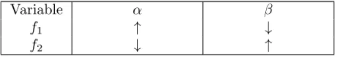
servicization strategy. . . 47 3.2 Comparative statics in Proposition 3 for f1 and f2. f1 and f2 are explicitly
stated in the proposition . . . 49 3.3 Equilibrium product durability, product use and firm profits under selling
strat-egy when the firm can sell two vertically differentiated products. . . 63 4.1 Equilibrium wholesale price . . . 76 A.1 Equilibrium when product quality is exogenously given . . . 85 A.2 Price Competition Equilibrium product quality, new and remanufactured
LIST OF FIGURES
2.1 Characterization of Equilibrium Regions . . . 15 2.2 Equilibrium new product quality and quantity (δ = 0.4, β = 1, Exogenous
qualitysf = 31β) . . . 16 2.3 Comparison of Social Surplus with NR and Exogenous Quality Benchmarks
(δ= 0.4,β = 1 and Exogenous qualitysf = 31β) . . . 19 2.4 Environmental Impact (e= 1, E= 3, δ= 0.5 in (a), α= 0.5 in (b)) . . . 22 2.5 Equilibrium quality when the OEM can collect and dispose the used cores (δ =
0.4, β= 1, h= 0.04) . . . 27 2.6 Equilibrium quality level when the IR incurs quality-independent cost(δ =
0.4, β= 1) . . . 32 2.7 Equilibrium quality and new product quantity when the perceptual quality gap
is independent of new product quality. ( α= 0.4, β= 1) . . . 34 3.1 Equilibrium regions under selling and servicization strategies. . . 47 3.2 The minimum operating efficiency above which servicization is more profitable
than selling strategy. (β = 0.3 in (a) and α= 0.8 in (b)) . . . 51 3.3 How servicization can improve environmental impact? . . . 59 3.4 When servicization can improve both profitability and environmental impact? . 60 3.5 Relative profititability of servicizing a single product to selling two differentiated
products. (α= 0.6) . . . 65 4.1 Firm A’s optimal supply chain structure and its responsibility decision when
externality is strongly negative. Dashed lines show the thresholds on fixed cost. (p= 3, w= 18, cr = 14, Q= 1, α=−13, β=−38) . . . 74 4.2 Firm A’s optimal supply chain structure and its responsibility decision when
externality is weakly negative or positive. (p= 3, w = 18, cr = 14, Q= 1, α=
1
3, β =−
3
8) . . . 75
4.3 Equilibrium when firm A can sell to firm B and f = 0. (p = 3, w = 18, cr =
1
4, Q= 1, β=−
3
8) . . . 77
(b) . . . 79 A.1 Comparison of Consumer and Social Surplus with NR and Exogenous Quality
Benchmarks when the OEM can collect and dispose used cores (α = 0.4, β= 1 and Exogenous quality sf = 31β) . . . 87 A.2 Comparison of Consumer and Social Surplus in Price competition with NR and
Exogenous Quality Benchmarks (δ= 0.4, β= 1 and Exogenous qualitysf = 31β) 87 A.3 Comparison of Consumer and Social Surplus with NR and Exogenous Quality
Benchmarks in the presence of quality independent remanufacturing cost (δ = 0.4, β= 1, n= 0.02 and Exogenous quality sf = 31β ) . . . 88 A.4 Comparison of Consumer and Social Surplus with NR and Exogenous Quality
Benchmarks in the presence of quality independent remanufacturing cost (δ = 0.4, β= 1, n= 0.06 and Exogenous quality sf = 31β ) . . . 89 A.5 Comparison of Consumer and Social Surplus with NR and Exogenous Quality
Benchmarks when the perceptual quality gap is independent of new product quality (α= 0.4, β= 1 and Exogenous qualitysf = 31β) . . . 90 B.1 Profit for the alternative operating cost. (θ = 2, c = 0.1, M = 1, α= 0.8, β =
0.3, mc= 0.1) . . . 101 B.2 Product durability for the alternative operating cost. (a) firm serves both
seg-ments under both selling servicization, and (b) low end segment is served only under servicization. (θ= 2, c= 0.1, M = 1, β= 0.3, mc= 0.10) . . . 101 B.3 Comparison of product durability for the alternative operating cost and the base
case. (θ= 2, c= 0.1, M = 1, α= 0.8, β= 0.3, mc= 0.1) . . . 102 B.4 Environmental impact for the alternative operating cost. (θ= 2, c = 0.1, M =
1, α= 0.8, β= 0.3, mc= 0.10, ep= 0.1, ed= 0.1) . . . 102 B.5 Consumer and Social Surplus for the alternative operating cost. (θ = 2, c =
CHAPTER 1
INTRODUCTION
In a globalized world, environmental and social impacts of business operations cannot be swept under the rug. Consumers are becoming more and more environmentally and so-cially conscious and demanding companies to follow environmentally and soso-cially sustainable practices. In this dissertation, we study the impact of several business operations on the environment and corporate social responsibility, and suggest sensible practices to reduce envi-ronmental impact and increase compliance levels with the envienvi-ronmental and labor standards. 1.1 Dissertation Overview
1.1.1 Competitive Quality Choice and Remanufacturing
reducing the environmental impact. Comparing our results with the benchmark in which the OEM remanufactures suggests that encouraging IRs to remanufacture in lieu of the OEMs may not benefit the environment. Furthermore, the benchmark illustrates that making re-manufacturing more attractive improves the environmental impact when the remanufacturer is the OEM, while worsening it when remanufacturing is done by the IR.
1.1.2 Is Servicization a Win-Win Strategy? Profitability and Environmen-tal Implications of Servicization
Servicization, a business strategy to sell the functionality of a product rather than the prod-uct itself, has been touted as a profitable and an environmentally friendly business practice. Profitability can increase because a firm can tailor the service to the needs of a customer. Envi-ronmental impact may be reduced because, under servicization, the firm retains the ownership and is responsible for the maintenance of the product. As a result, the firm has stronger incen-tives to invest in product durability. Motivated by these dynamics, we analytically characterize when servicization can simultaneously increase a firm’s profits and decrease its environmental impact compared to selling products. We endogenize the firm’s product durability and pricing decisions, as well as the customer’s level of use of a product. We allow for heterogeneous customer segments with differing product valuations, and capture the difference in product operating cost incurred by the firm and by the customer.
implemented with care.
1.1.3 Responsible sourcing via vertical integration: the impacts of scrutiny, demand externality, and cross sourcing
As outsourcing to emerging economies have increased, many unfortunate events about the practices in those countries hit the news channels. These includes but not limited to collapse of the Rana Plaza factory in Bangladesh (New York Times, 2013), allegations of sweatshop and child labor at factories of Nike suppliers (Daily Mail, 2011). Companies outsource from emerging economies mainly because the lower operating and labor costs. However, many times this cost advantage comes at the expense of social responsibility compliance. Suppliers may engage in unethical practices to lower costs and squeeze more profits. Insufficient regulations in these countries also fuel noncompliance.
In this chapter, we investigate vertical integration as a way to ensure compliance in a com-petitive setting. One of the firms is capable of vertical integration and chooses to comply/not comply with the environmental and labor standards, whichever is more profitable. If at least one of the firms does not comply with the law, with positive probability it will get caught and lose a portion of its demand. This may have positive or negative impact on the other firm. The impact may be positive because a portion of the consumers exited the firm caught with a violation may purchase from the other firm. On the other hand, it may be negative because the violation publicity may tarnish the image of entire industry.
CHAPTER 2
COMPETITIVE QUALITY CHOICE AND REMANUFACTURING
2.1 Introduction
Remanufacturing operations involve taking used products, bringing them back to as-new condi-tion, and selling them again (Atasu et al., 2010). These activities in an industry can be carried out either by third-party independent remanufacturers (IR) or by original equipment manu-facturers (OEM). Especially in the US, majority of remanufacturing is done by IRs (Hauser and Lund, 2008). The same study finds that the remanufacturing industry in the U.S. is worth $53 billion, which means that IRs are not an insignificant competitive threat to OEMs. OEMs try to fend off competition from IRs through limiting quantity, specifically by creating scarcity of cores available for remanufacturing (e.g., by offering free take-back of cores from consumers (HP 2010a) or making cores ineligible for remanufacturing (Lexmark 2010)) and rarely through litigation (e.g., HP 2010b).
it also increases the quality of the remanufactured product to a certain extent. Therefore, the results on product quality from papers that consider competition between independent
products (e.g., Moorthy 1988; Desai 2001) do not immediately extend to the remanufacturing context. Thus, in this paper we studyhow an OEM can use product quality along with quantity as a competitive lever against an IR.
Remanufacturing is generally perceived as an environmentally-friendly end-of-use man-agement option for many products. Commonly-cited benefits include diversion of discarded products from landfills, reduced virgin raw material usage and reduced energy usage when compared to manufacturing (U.S.EPA, 1997). At the same time, Gutowski et al. (2011) find that while remanufacturing itself uses less energy than manufacturing, remanufactured products may be less energy efficient. Thus, the relative environmental impacts of new and remanufactured products should be carefully considered and the total environmental impact of remanufacturing in a given market is not clear.
Recently, we have seen a surge of activities that promote remanufacturing. For example, the Automobile Parts Remanufacturers Association introduced the Recycling/Remanufacturing Tax Credit Bill, HR 5695 (The Remanufacturing Institute, 2008) and campaigns such as Man-ufactured Again (Motor and Equipment Remanufacturers Association 2011) work to increase remanufacturing levels by increasing consumer awareness. An underlying tenet of these activ-ities is that remanufacturing is good for the consumer. However, just like total environmental impact, the social welfare implications of remanufacturing, especially when it is conducted by a third-party are not well understood. To this end, we research how the competition between the IR and the OEM affects total environmental impact and social welfare, specifically when the OEM can adjust product quality in response to competition.
the OEM sells the new product and remanufacturing is done solely by the IR. In addition to our base model, we consider several benchmarks: a monopolist OEM without remanufac-turing capability (NR benchmark), a monopolist OEM with remanufacremanufac-turing capability, and competition with exogenous quality decision. These benchmarks help tease out the effects of competition, the OEM’s quality choice and the type of the remanufacturing firm on our results.
Even though most remanufacturing in the US is done by IRs, OEMs like Xerox, Kodak and Caterpillar have remanufacturing operations, too. In an extension to our base model, we study how the answers to our research questions change when the OEM remanufactures instead of the IR. Comparing our findings with the results of this extension, we are able to provide insights on how the environmental and social welfare benefits of remanufacturing depend on thetype of company (IR vs. OEM) offering the remanufactured product. When faced with competition from an IR, some OEMs like Lexmark choose to collect cores and dispose of them rather than remanufacture in-house. We analyze this scenario as an extension to our base model as well and provide insights regarding when the OEM prefers to collect cores to compete with the IR. We now summarize our key findings:
•We explicitly characterize how the OEM competes with the IR in equilibrium. When the OEM has a significant competitive advantage (which is determined by the relative cost and the perceived quality of the remanufactured product vis-a-vis the new product and is explained in detail in Section 2.3), it deters the IR’s entry by choosing a quality level that is higher than it would if the IR was not in the market. In contrast, when the IR has a significant competitive advantage, the OEM reduces production and, hence, decreases the number of cores the IR can remanufacture. In between, the IR enters the market and does not encounter core shortage. In this region, when the OEM has the competitive advantage, it chooses a higher quality level compared to the NR benchmark to emphasize its advantage. When the IR has the competitive advantage, the OEM chooses a lower quality level to de-emphasize its competitor’s advantage. Our results show that when the OEM has a stronger competitive position, it is more likely rely on quality as a strategic lever whereas when the IR’s competitive position gets stronger, the OEM is more likely to rely on limiting core availability.
compared to the NR benchmark; that is, remanufacturing may harm consumer welfare. This is because the OEM chooses an inefficiently high quality level to deter or weaken the IR. In contrast, when the product quality is exogenously fixed, the consumer surplus always increases with remanufacturing. We show a similar result for the social surplus. These results are in contrast with our monopoly remanufacturing benchmark which shows remanufacturing by an OEM always benefits the consumer and social surplus. There are two factors in play here: (i) An IR chooses to remanufacture even when the perceived value to cost ratio of the remanufactured product is unfavorable relative to the new product. In other words, the OEM’s remanufacturing incentives are better aligned with consumer and social surplus than that of the IR. (ii) When the OEM remanufactures itself, it chooses product quality more efficiently as far as consumer and social surplus are concerned. Overall, our results illustrate that ignoring competition or OEM’s quality choice lead to overestimating benefits of remanufacturing for consumer and social welfare.
encouraging IRs to remanufacture.
•For the two alternative models we consider, in which the OEM can also remanufacture or it can preemptively collect cores, we show through numerical studies that the way the OEM chooses to compete with the IR is similar to our base model. Consistent with our insights from the base model, the OEM follows a deterrent quality strategy when remanufacturing does not have a strong value proposition; in contrast, it uses a deterrent quantity strategy (remanufacturing itself or collecting cores and disposing of them) when the IR’s remanufactur-ing becomes a bigger threat. Furthermore, we find makremanufactur-ing remanufacturremanufactur-ing more attractive, by either lower cost or higher quality perception, can worsen the environmental impact when remanufacturing is done by the IR; in contrast it lessens the environmental impact when the OEM is remanufacturing. Thus, the consequences of these incentives on environmental impact critically depend on the type of the remanufacturing firm.
• We demonstrate the robustness of the equilibrium structure, which shows how the OEM chooses to compete with the IR, under three different extensions: the IR incurs an additional cost independent of the quality level; perceptual quality gap between new and remanufac-tured products is independent of product quality; the OEM and the IR compete in prices. Comparison of our results from the base model and the extensions, however, shows that the effect of IR’s competitive threat on the OEM’s quality choice may critically depend on how the cost and perceived quality of the remanufactured product are modeled. Furthermore, the implication of remanufacturing on the social and consumer surplus and environmental impact can be sensitive to the type of competition (price vs. quantity).
2.2 Literature Review
of an OEM, the profitability of introducing a remanufactured product versus collecting and disposing of used products to deter the entry of an IR. This stream of literature studies how the competition between new and remanufactured products affects the pricing and quantity decisions of the OEM (a feature that also exists in our model) but does not capture the OEM’s
endogenous quality decision. We extend this literature by allowing the OEM to explicitly set product quality. We characterize how the OEM uses two modes of competition–quality and quantity–as its competitive position vis-a-vis the IR changes. We also research how the competition between an OEM and an IR and the OEM’s ability to choose the quality level affect consumer surplus and the product’s total environmental impact.
How competition affects a firm’s quality choice has been studied extensively in marketing literature. One fundamental difference of our model is that the OEM makes the quality decision and its decision locks in the quality of the remanufactured product whereas in the extant literature, competing firms are allowed to choose their own quality levels independently. This difference leads to significantly different insights. For example, Moorthy (1988) shows that in a duopoly when firms choose their quality levels first and then compete in prices, consumer surplus is higher than the monopoly case. In our model, consumer surplus may be lower than the monopoly case because the OEM takes advantage of the interdependency between the products and may inefficiently increase or decrease quality in order to weaken the IR’s competitive position. Desai (2001) also models a duopoly but with symmetric firms. In contrast, the asymmetry between the OEM and the IR determine their relative competitive positioning which plays a key role in our results.
our model quality is an intrinsic product attribute independent of the magnitude of demand. We study competitive quality choice for a remanufacturable product. Quality is an impor-tant product design decision and has been of great interest in the new product development literature (e.g., Souza et al. 2004; Plambeck and Wang 2009; Fishman and Rob 2000). How-ever, these papers are mainly concerned with sequential quality improvements whereas quality choice is made only once in our model. Furthermore, the remanufacturing context has some unique aspects: the remanufactured product’s cost and quality level depend on the new prod-uct’s quality level and the OEM can limit the cores that the IR can access for remanufacturing, which adds another layer of interdependence. Here, we contribute by studying quality choice for a product that competes with an interrelated product.
In the context of product recovery, few papers consider product quality explicitly. In Debo et al. (2005) and Robotis et al. (2009), quality refers to the remanufacturability level of the returned product, which reduces the remanufacturing cost; this is different from our definition. Debo et al. (2005) model a monopolist OEM and research whether the OEM should sell a remanufacturable product and if so, what the level of remanufacturability should be. In an extension that allows competition with IRs, they find that as remanufacturing competition intensifies, the remanufacturability level of the product goes down. However, we find that as the IR becomes more competitive up to a threshold level, product quality goes up. Robotis et al. (2009) consider a monopolist and show uncertainty in remanufacturing cost may lead to higher reusability investment. Subramanian et al. (2011) study how remanufacturing threat of an IR affects component commonality decision for an OEM selling two vertically differentiated products with exogenous qualities.
this work, we confine ourselves to a single recovery form, i.e., remanufacturing, but consider the competition between the OEM and the IR. We also study how the product quality level and benefits of remanufacturing depend on the party (OEM or IR) doing the remanufactur-ing. We find that when an OEM and an independent remanufacturer are in competition, remanufacturing may indeed result in decreased quality and increased environmental impact.
2.3 Model
We consider an original equipment manufacturer (OEM) selling a new product and an inde-pendent remanufacturer (IR) selling the remanufactured product. We begin by introducing the demand model, discuss the cost structure and finally describe the firms’ decisions.
Each customer considers new product, remanufactured product and no purchase options and chooses the one that maximizes her utility. We model consumer preferences as in Moorthy (1988). Consumers are heterogeneous in their willingness to pay for quality and are uniformly distributed over a bounded support with unit density, which we normalize to [0,1]. A consumer of typeθ∈[0,1] is willing to payθsfor a product of quality levels. This implies that everything else being equal all consumers prefer higher quality over lower quality. Given that pn is the new product’s price, the utility a type θ customer receives from the new product is θs−pn. Consumers often perceive the remanufactured product as being of inferior quality. We capture this by modeling consumers’ willingness to pay for the remanufactured product as aδ fraction of the new product where δ ∈ (0,1). Consumption of the remanufactured product provides a utility of δθs−pr where pr is the remanufactured product’s price. This implies that the quality gap between the new and remanufactured products is proportional to product quality
s. Among others, Ferguson and Toktay (2006) and Atasu et al. (2008) model demand and the relative valuation of the remanufactured product similarly. In Section 2.8.3, we consider an alternative model where the quality gap is independent of product quality.
product. At the same time, remanufacturing a product costs less than manufacturing a product because some parts are reused. The remanufacturing cost is proportional to the cost of new product, specifically, it is equal toβαs2. As such, our base model does not consider a quality-independent cost term. An extension in section 2.8.2 allows for such an additional cost term as in Atasu and Souza (2012). Here, α ∈ (0,1) is an indicator of the remanufacturing cost advantage and it decreases as the cost savings from remanufacturing increases. Like Debo et al. (2005) and Ferrer and Swaminathan (2006), we assume that the remanufacturing cost subsumes the cost of all remanufacturing related activities.
The order of decisions is as follows. First, the OEM decides the quality of the product s. Then the OEM and the IR competitively choose new product and remanufactured product quantities, qn and qr that are sold in a single period. The IR’s remanufacturing quantity is constrained by the available cores, which is determined by the new product quantity. The IR can also choose to stay out of the competition by choosing to remanufacture zero units. Finally, consumers make their choices.
We consider a product that has a single (long) life and the quality decision is made at the beginning of this long life cycle. Single period models have previously been used in Atasu and Souza (2012); Agrawal et al. (2011a); Subramanian et al. (2011) in the sustainable operations management literature. This approach, which focuses on steady state profits, facilitates ana-lytical tractability in our model and allows us to focus on our research questions. Furthermore, the OEM and IR engage in Cournot type quantity competition in our model as in Ferguson and Toktay (2006); Debo et al. (2005); Atasu et al. (2009a). Both quantity and price competi-tion models are extensively used in the OM literature. While our base model adopts quantity competition, we also study price competition showing that our equilibrium results propagate. Following Johnson and Myatt (2006), the OEM’s and the IR’s chosen quantities and cus-tomer choices lead to following prices for the new and remanufactured products:
pn=s(1−qn−δqr), pr =δs(1−qn−qr).
(e.g., Atasu and Souza 2012; Debo et al. 2005; Ferguson and Toktay 2006). Our model can be extended such that only a fraction of the cores is available for remanufacturing, but for tractability and to keep the focus on our research question, we only consider the case where all cores can be remanufactured.
We derive the equilibrium by backward induction. For a given quality level s, the OEM and the IR play the quantity game. Formally, the OEM solves
max qn
πOEM(qn|s) = [s(1−qn−δqr)−βs2]qn
s.t qn≥0
and the IR simultaneously solves
max qr
πIR(qr|s) = [δs(1−qn−qr)−αβs2]qr
s.t qr≥0, qr ≤qn.
This solution approach is the same as in Agrawal et al. (2011a). The IR’s problem has an ad-ditional constraint reflecting the fact that the remanufactured product quantity cannot exceed the new product quantity, i.e.,qr ≤qn, core availability constraint. Finally, the OEM chooses the optimal quality level s∗ by solving maxsπOEM(s|q∗n(s), qr∗(s)). The resulting equilibrium is described in the next section. Note that we use the superscript (*) to denote equilibrium values throughout the paper.
results. The equilibria for the benchmarks and all the proofs are provided in Appendix A.
2.4 Equilibrium
In this section, we discuss the decisions of the OEM and the IR in equilibrium. As it will be evident, remanufactured product’s relative cost-to-value ratio, α/δ, simply referred to as the cost-to-value ratio plays an important role in our result. When α/δ ratio decreases, the IR’s competitiveness increases and vice versa for the OEM. This is because increasing α/δ
ratio indicates either the cost of remanufacturing goes up or the consumer perception of the remanufactured product goes down. Specifically, when α/δ is greater than 1, the OEM has the cost-to-value advantage against the IR. In contrast, when the cost-to-value ratio is smaller than 1, the IR has the advantage. Consider medical imaging equipments and printer cartridges for two examples that fall on two opposite ends of the spectrum. Remanufacturing medical imaging equipments (e.g., computer tomography and magnetic resonance imaging) have a high marginal cost due to high technology components used in these products. In addition, hospitals are skeptical about buying remanufactured imaging devices (Elsberry, 2002) since they can have a direct impact on patients’ health. Thus, medical imaging equipments can be characterized by a large α/δ ratio. In contrast, printer cartridges possess a small α/δ ratio due to low cost and high consumer acceptance of remanufactured cartridges. In fact, cartridge industry is one of the prominent examples where the competition between the IRs and the OEMs (e.g., Lexmark, HP) is very severe. The next proposition describes the equilibrium.
Proposition 1. The following characterizes the equilibrium regions. The equilibrium quality, new and remanufactured product quantities are provided in Table 2.1.
R1. If αδ ≥2, the IR cannot enter the market and the OEM acts like a monopoly.
R2. If 84+−δδ ≤ αδ <2, the IR is a threat and its entry is deterred by the OEM.
R3. If δ(18−(48δ−−δ2)δ22+δ3) <
α δ <
8−δ
4+δ, the IR enters the market but does not remanufacture all
available cores.
0 0.1 0.2 0.3 0.4 0.5 0.6 0.7 0.8 0.9 1 0
0.1 0.2 0.3 0.4 0.5 0.6 0.7 0.8 0.9 1
α
δ
R4
R3
R2
R1
Figure 2.1: Characterization of Equilibrium Regions
Region s∗ q∗n q∗r
R1 31β 13 0
R2 δ
β(2α−δ)
α−δ
2α−δ 0
R3 3β2(2−−δα) 2(23(4−−δδ)) (83(2−δ−)δα−)(4α(4+−δ)δδ)
R4 1
3β
2 3(2+δ)
2 3(2+δ)
Table 2.1: Equilibrium product quality, and new and remanufactured product quantities
Figure 2.1 graphically depicts the equilibrium regions in the Proposition. Note that the cost-to-value advantage shifts from the OEM to the IR as we move from region R1 to R4. In region R1, the IR does not pose a threat due to its severe cost-to-value disadvantage and the OEM acts as a monopolist leading to the same outcome as the NR benchmark.
In region R2, the IR is a competitive threat. However, the OEM is able to deter entry by choosing a higher level of quality compared to the NR benchmark. Because the quality of the new product directly impacts its remanufacturing cost, by increasing quality the OEM also increases the cost of remanufacturing. Thus, the IR cannot recover its cost due to its significant cost-to-value disadvantage and stays out of the market. Table 2.1 shows that the OEM needs to increase quality to deter entry when the IR becomes a bigger threat as a result of more favorable cost-to-value ratio. Figure 2.2a graphically demonstrates how the OEM’s chosen quality level depends on the IR’s cost of remanufacturing. We refer to the OEM’s behavior in region R2 as entry deterrence because the OEM prevents the IR’s entry by deviating from the NR benchmark. Note that entry deterrence does not exist in the exogenous quality benchmark (see Section A.1). In other words, quantity alone is not sufficient to deter entry.
0 0.1 0.2 0.3 0.4 0.5 0.6 0.7 0.8 0.9 1 0.3
0.32 0.34 0.36 0.38 0.4 0.42
α
Product Quality
R4 R3 R2 R1
No−reman. Base model
(a) Quality
0 0.1 0.2 0.3 0.4 0.5 0.6 0.7 0.8 0.9 1 0.27
0.28 0.29 0.3 0.31 0.32 0.33 0.34
α
New Product Quantity
R4 R3 R2 R1
No−reman. Exogenous Base model
(b) New Product Quantity
Figure 2.2: Equilibrium new product quality and quantity (δ= 0.4,β = 1, Exogenous quality
sf = 31β)
choose a higher or lower quality level when compared to the NR benchmark depending on who has the cost-to-value advantage. When the OEM has the cost-to-value advantage, i.e.,
α
δ >1, it chooses a higher quality level. In this case, increasing product quality increases the remanufacturing cost but customer perception of remanufactured product does not increase proportionally, which in turn weakens the IR’s competitive position. In contrast, when IR has the cost-to-value advantage, i.e., αδ <1, the OEM chooses a lower quality level to de-emphasize its competitor’s advantage.
between strategies.
Proposition 1 demonstrates when the IR has a significant cost-to-value advantage, the OEM focuses primarily on a quantity limiting strategy. Indeed, this is consistent what we see in the printer cartridge industry where IRs have a significant cost-to-value advantage and OEMs mostly try to compete with IRs by creating quantity scarcity.
Proposition 1 illustrates that when the OEM has the cost-to-value advantage it relies more on the quality lever whereas when the advantage shifts to the IR, it increasingly relies on the quantity lever. Regions R2 and R4 demonstrate two extremes. In R2, the OEM has a significant cost-to-value advantage, and it relies solely on quality to deter the IR’s entry (the OEM’s quantity is the monopoly quantity given its chosen quality). In contrast inR4, the IR has a significant cost-to-value advantage, and the OEM uses only the quantity lever in this case keeping its quality at the NR benchmark level.
It is worthwhile to contrast our findings with the monopoly remanufacturing benchmark. A monopolist always increases its chosen product quality after engaging in remanufacturing (Details of the analysis are provided in section A.1.2). In contrast, when remanufacturing is performed by the IR, the OEM can decrease product quality compared to the NR benchmark. This happens because the OEM’s quality decision directly affects the IR’s competitive position while a monopolist OEM who remanufactures in-house does not need to worry about a com-petitor. When faced with competition from an IR, the OEM needs to take into account who has the cost-to-value advantage when making its quality decision. Under different modeling assumptions, Atasu and Souza (2012) also find that a monopolist OEM engaging in quality recovery (of which remanufacturing is an example) chooses a quality level that is weakly higher than the no-recovery scenario.
2.5 Consumer and Social Welfare
In this section we investigate the impact of remanufacturing and quality choice on consumer surplus (CS) and social surplus (SS). The consumer surplus is given by
CS=
Z 1−qn
1−qn−qr
(δθs−pr)dθ+
Z 1
1−qn
where the first term is the surplus from remanufactured products, and the second term is the surplus from new products sold. The social surplus is the sum of the consumer surplus and the firm profits.
Intuition suggests remanufacturing should improve consumer welfare. Indeed, the next proposition confirms this conjecture for the exogenous quality benchmark, that is, when the OEM responds to the IR’s entry only with its quantity keeping its quality constant.
Proposition 2. IR’s entry always increases CS in the exogenous quality benchmark.
However, the OEM does not keep its product quality constant when faced with the IR threat. Proposition 1 shows how the OEM adjusts its product quality to strengthen its com-petitive position. Basically, it may choose lower or higher quality levels depending on its cost-to-value position relative to the IR. The next proposition demonstrates remanufacturing can hurt CS due to the OEM’s quality choice.
Proposition 3. There exists αc satisfying 1 < αδc < 84+−δδ such that CS is higher than that of
the NR benchmark if and only if α < αc. Furthermore, CS is strictly smaller than that of the
NR benchmark when αc
δ < α δ <2. Propositions 1 and 3 show αc
δ falls in region R3. Thus, CS is lower than or equal to the NR benchmark in regions R1 and R2. In region R1, the IR is not a threat and the outcome is identical to the NR benchmark. In region R2, however, CS is strictly smaller than that of the NR benchmark as shown in the second half of the proposition. Specifically, in region
R2, the OEM inefficiently chooses higher quality to deter the IR’s entry, therefore focuses on the higher valuation consumers which in turn reduces CS. Interestingly, CS can also suffer in regionR3 even when the IR enters the market. This is again due to the OEM’s choice of high quality to play to its cost-to-value advantage.
overestimating the benefit of remanufacturing for consumers. Now let us consider the impact of remanufacturing on social surplus.
Proposition 4. There exists αs satisfying 1 < αδs < 84+−δδ such that SS is higher than that of
the NR benchmark if and only if α < αs. Furthermore, SS is strictly smaller than that of the
NR benchmark when αs
δ < α δ <2.
0.45 0.5 0.55 0.6 0.65 0.7 0.75 0.8
0.0535 0.054 0.0545 0.055 0.0555 0.056 0.0565 0.057
R3 R2
α
Social Surplus
No−reman. Exogenous Base model
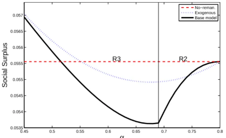
Figure 2.3: Comparison of Social Surplus with NR and Exogenous Quality Benchmarks (δ = 0.4,β = 1 and Exogenous qualitysf = 31β)
The proposition indicates that the IR’s entry threat as well as its successful entry can de-crease not only CS but also SS when the IR’s cost-to-value position is not sufficiently favorable. Figure 2.3 compares SS against the NR and exogenous quality benchmarks. In the exogenous quality benchmark, the new product quality is kept at the NR benchmark quality disregarding the OEM’s quality response to the IR threat. When the IR remanufactures, SS is always lower than the exogenous quality benchmark. Furthermore, note that when 0.516< α <0.55, remanufacturing worsens SS in our base model while improving it in the exogenous quality benchmark. In this case, ignoring the OEM’s quality decision leads to incorrectly concluding that remanufacturing would benefit social welfare.
a very attractive cost-to-value position. The OEM would not choose to remanufacture in regions in which the IR’s remanufacturing decreases CS and SS.1 In other words, the OEM’s remanufacturing incentives are better aligned with consumer and social welfare compared to the IR’s. Second, when the OEM utilizes the benefits of remanufacturing, it chooses product quality more efficiently as far as CS and SS are concerned. In contrast, when an IR does the remanufacturing, the OEM can inefficiently increase quality to deter entry or decrease quality to undermine the cost-to-value advantage of its competitor.
Our findings have important policy implications. There is an ongoing policy debate whether and when to promote remanufacturing. For example, the Recycling/Remanufacturing Tax Credit Bill, HR 5695 (The Remanufacturing Institute, 2008) introduced by the Automobile Parts Remanufacturers Association (APRA) calls for tax credits for investments in remanufac-turing equipment. Although the bill did not pass the first time round, efforts to pass it continue. Similarly, the Waste Electrical and Electronic Equipment (WEEE) Directive legislation in the European Union holds manufacturers financially responsible for taking back and disposing of end-of-life electric and electronic equipment. In a recent vote on changes to the directive, a 5% reuse target was introduced to promote higher levels of reuse/remanufacturing (Jowitt, 2011). In addition, environmental awareness campaigns, companies promoting sustainable business practices, etc. may work to improve customers’ perception of remanufactured products. Such incentives and campaigns can alter competitive positioning of IRs and OEMs and change their behavior. Our findings illustrate policy makers should be careful when designing such incen-tives especially when IRs (rather than OEMs themselves) engage in remanufacturing. Making remanufacturing attractive for IRs does not necessarily improve social welfare. Propositions 3 and 4 show that the IR’s threat and entry can decrease both CS and SS. Furthermore, ignoring competition or the OEM’s quality decision can lead to overestimating benefits of remanufacturing for consumer and social surplus.
1
Region α δ
R1 Constant Constant
R2 ↑ ↓
R3 ↓ Concave(if Ee <1),↑(if Ee >1)
R4 Constant ↓
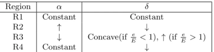
Table 2.2: Environmental impact comparative statics
2.6 Environmental Impact
We follow the convention in the literature (Atasu and Souza, 2012; Agrawal et al., 2011b; White et al., 1999), and assume that one unit of new product and remanufactured product entail E and e environmental impact respectively considering all stages of product life cycle which includes production, use by customers, end of life and remanufacturing. Therefore, when the OEM producesqn units and the IR remanufacturesqr units, the total environmental impact isqnE+qre.
Next proposition shows the effect of remanufacturing on the environment comparing it the NR benchmark and describes how environmental impact depends on relative cost α and perception δ of the remanufactured product.
Proposition 5. Table 2.2 shows how the environmental impact changes withα and δ. • When the IR is not a threat (region R1), the environmental impact is the same as the
NR benchmark level.
• When the IR’s entry is deterred by the OEM (region R2), the environmental impact is always lower than the NR benchmark level.
• When the IR enters the market but does not remanufacture all available cores (region
R3), the environmental impact is lower than the NR benchmark level if and only if
e E <
(−2+α)δ2
(−8+δ)δ+α(4+δ).
• When the IR enters the market and remanufactures all available cores (region R4), the environmental impact is lower than the NR benchmark level if and only if Ee < δ2.
customers, which in turn decreases the quantity sold. Furthermore, Table 2.2 shows that as the IR becomes a bigger threat, the environmental impact decreases further in this region since the OEM needs to keep increasing quality to deter entry as the IR’s cost-to-value position improves.
The IR remanufactures in regionsR3 andR4 and the relative impact of new and remanufac-tured products Ee determines the environmental impact of remanufacturing in these regions. Specifically, when remanufactured product has a sufficiently smaller relative environmental impact indicating small Ee, the overall environmental impact decreases with the IR’s entry. Otherwise, remanufacturing increases the environmental impact.
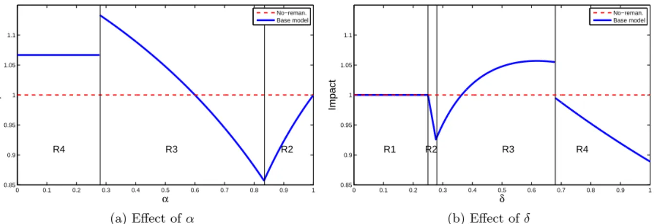
Figure 2.4 illustrates how the environmental impact depends on the IR’s relative competi-tive position showing that environmental impact attains its worst level in region R3. This is because competition between the IR and the OEM is more intense yielding more quantity sold (new + remanufactured) when neither has a significant cost-to-value advantage. The environ-mental impact gets smaller near region R2, as the OEM’s cost-to-value advantage improves. Similarly at the other end, the environmental impact is also smaller in region R4, where the IR has a significant cost-to-value advantage.2
0 0.1 0.2 0.3 0.4 0.5 0.6 0.7 0.8 0.9 1 0.85
0.9 0.95 1 1.05 1.1
α
Impact
R4 R3 R2
No−reman. Base model
(a) Effect ofα
0 0.1 0.2 0.3 0.4 0.5 0.6 0.7 0.8 0.9 1 0.85
0.9 0.95 1 1.05 1.1
δ
Impact
R1 R2 R3 R4
No−reman. Base model
(b) Effect ofδ
Figure 2.4: Environmental Impact (e= 1,E = 3,δ = 0.5 in (a),α= 0.5 in (b))
In regionR4, the OEM follows the quantity scarcity policy to limit the IR’s remanufactur-ing. Table 2.2 shows that when the IR’s cost-to-value position gets even better due to a higher
δ in this region, the OEM further decreases its quantity, benefiting the environmental impact.
Both in regions R2 and R4, quantity hence the environmental impact decreases when the IR becomes more powerful. But there are different dynamics in place. InR2, quantity decreases because the OEM increases quality to deter the IR, whereas in region R4, the OEM creates scarcity to limit the IR’s remanufacturing.
Comparisons with the monopoly remanufacturing benchmark (see section A.1.2 for details) show that how remanufacturing changes the environmental impact level depends on who— OEM or IR—does the remanufacturing. We find that if remanufacturing has the cost-to-value advantage (αδ <1), and hence, is socially desirable3, whenever the environmental impact in the base model is smaller than the NR benchmark, environmental impact in the monopoly re-manufacturing benchmark is also smaller than the NR benchmark but not vice versa. Hence, remanufacturing by an OEM is more likely to decrease environmental impact than remanufac-turing by an IR (Our extension in Section 2.7.1 finds a similar result). This is mainly due to two factors: (i) Competition increases the total quantity sold; a monopoly always sells fewer units. (ii) The OEM can reduce the quality level when the competing IR has the cost-to-value advantage and a lower quality level implies a bigger quantity in the market. Under somewhat different modeling assumptions, Atasu and Souza (2012) find that quality recovery (of which remanufacturing is an example) carried out by a monopolistic OEM always decreases the en-vironmental impact, which is also in contrast with our base model. Our findings together with Atasu and Souza (2012) suggest that as far as the environmental impact is concerned, it may not be beneficial to encourage IRs rather than OEMs to remanufacture. Furthermore, when an IR does the remanufacturing, increased competition can aggravate environmental impact. In this case, it is desirable to have an IR with either a sufficiently unfavorable cost-to-value ratio so the OEM increases the quality level or a sufficiently favorable cost-to-value ratio so the OEM competes by creating quantity scarcity.
3
We know from section 2.5 and section A.1.2 that in both the base model and the monopoly remanufacturing
benchmark, CS and SS levels are higher than the NR benchmark when αδ <1. In addition, in the monopoly
δ s∗ q∗n qmr∗ q∗ir CS SS e/E
0.40 0.333 0.333 0 0 0.0185 0.0556 −
0.43 0.368 0.316 0 0 0.0184 0.0551 ∞
0.46 0.403 0.298 0 0 0.0179 0.0538 ∞
0.49 0.419 0.287 0 0.014 0.0181 0.0516 3.278 0.52 0.411 0.284 0 0.042 0.0193 0.0527 1.186 0.55 0.403 0.280 0 0.067 0.0205 0.0531 0.793 0.58 0.394 0.277 0 0.090 0.0217 0.0538 0.631 0.61 0.298 0.190 0.190 0 0.0152 0.0455 0.758 0.64 0.304 0.187 0.187 0 0.0155 0.0466 0.780 0.67 0.309 0.185 0.185 0 0.0159 0.0478 0.802
δ s∗ qn∗ q∗mr q∗ir CS SS e/E
0.70 0.315 0.183 0.183 0 0.0163 0.0489 0.824 0.73 0.320 0.181 0.181 0 0.0167 0.0501 0.844 0.76 0.326 0.179 0.179 0 0.0171 0.0513 0.863 0.79 0.331 0.177 0.177 0 0.0175 0.0525 0.883 0.82 0.333 0.175 0.175 0 0.0179 0.0538 0.901 0.85 0.345 0.174 0.174 0 0.0183 0.0550 0.919 0.88 0.348 0.172 0.172 0 0.0188 0.0563 0.936 0.91 0.354 0.171 0.171 0 0.0192 0.0577 0.953 0.94 0.359 0.169 0.169 0 0.0197 0.0590 0.969 0.97 0.365 0.168 0.168 0 0.0201 0.0603 0.974
Table 2.3: Equilibrium and the resulting consumer/social surplus and environmental impact when the OEM can also remanufacture (β= 1, α= 0.8)
2.7 Additional Competitive Levers
In this section we study two additional levers an OEM can use to compete with an IR. Specif-ically, the OEM can also remanufacture its own product or it can collect cores to make them unavailable for the IR.
2.7.1 Remanufacturing by both OEM and IR
Remanufacturing can be done by IRs as well as by the OEM itself. There are examples of both in practice. For example, Xerox leases its copiers and remanufactures end-of-lease copiers by itself; in contrast in the cartridge industry mainly IRs do the remanufacturing. Here, we extend our base model and allow the OEM to remanufacture its own product in addition to the IR. We conduct a numerical study to analyze the resulting equilibrium.
The OEM and the IR have the same remanufacturing cost (βαs2 in our model) and they choose their desired remanufacturing quantities simultaneously. However, the OEM has the priority in quantity allocation when their total demand exceeds the number of available cores. In other words, the IR can remanufacture only the cores that the OEM chooses not to re-manufacture. Admittedly, this approach favors OEM’s remanufacturing, but even with this bias, we show the OEM may prefer letting the IR remanufacture and instead continue to com-pete through manipulating quality. Note the other extreme where the IR gets priority in the allocation of available cores results in the same equilibrium outcome as our base model.4
4Essentially, in this scenario, any core that is not profitable for the IR to remanufacture is not profitable for
Table 2.3 reports results of our numerical study as δ varies for one α value, α = 0.8. In our study, we repeat the same analysis for α ∈ {0.1,0.2,0.3,0.4,0.5,0.6,0.7,0.8,0.9} values and find that Table 2.3 is representative of their outcomes as well. Quality cost coefficient
β is a scale factor in our model and it is kept at β = 1. In the table, qmr and qir show the number of remanufactured units by the OEM and the IR, respectively. Furthermore, e/E
shows the maximum e/E ratio–environmental impact of remanufactured product relative the new product–below which remanufacturing (or the possibility of it) reduces environmental impact compared to the NR benchmark. In the Table e/E is not reported for δ = 0.4 since whenδ ≤0.4, remanufacturing is not viable, and the NR benchmark and our extended model yields the same outcome.
To better understand the effect of competition, consider the OEM’s optimal policy in the absence of an IR. A monopolist OEM does not remanufacture when the cost-to-value ratio favors the new product, i.e.,α/δ >1. It remanufactures some but not all available cores when the remanufactured product has the cost-to-value advantage, i.e.,α/δ <1 but the advantage is not sufficiently big (0.8< δ <0.9 in Table 2.3). Finally, when the remanufactured product has a significant cost-to-value advantage, a monopolist OEM remanufactures all available cores. Table 2.3 shows when remanufacturing has a sufficiently big advantage or disadvantage, the OEM does not need to deviate from the monopoly optimal policy to compete with the IR. Specifically, when remanufacturing has a severe disadvantage (δ ≤0.4), the IR is not a threat, the OEM sells only the new product. In contrast, when remanufacturing has a significant advantage (δ≥0.91), the OEM remanufactures all available cores leaving no cores to the IR. When cost-to-value ratio of remanufacturingα/δis moderate (0.4< δ≤0.88 in Table 2.3), the OEM needs to actively compete with the IR. The OEM uses different policies depending on the cost-to-value position of remanufacturing. Note remanufacturing becomes increasingly attractive asδ increases. When 0.40< δ <0.49, similar to our base model, the OEM increases quality to deter the IR from remanufacturing. When 0.49 ≤ δ < 0.61, the OEM lets the IR remanufacture but it increases quality to weaken the IR’s competitive position. It is interesting that the OEM is using only quality as a strategic lever in 0.40 < δ <0.61 although our core
allocation gives absolute priority to the OEM. Finally, the OEM inefficiently remanufactures
all available cores itself in order to leave no cores available to the IR when 0.61≤ δ ≤ 0.81. This discussion demonstrates that similar to our base model, the OEM relies on quality as a competitive lever when remanufacturing does not have a strong cost-to-value position, in contrast, it uses a quantity limiting strategy when the IR’s remanufacturing becomes a bigger threat.
The OEM increases quality when the remanufactured product has the cost-to-value ad-vantage, i.e, α/δ < 1. This is in direct contrast to the base model. Essentially, when the OEM itself rather than a competitor IR does the remanufacturing, the OEM is better off underscoring the remanufactured product’s advantage by increasing quality. However, when the remanufactured product has the disadvantage, i.e.,α/δ >1 and the OEM remanufactures solely to eliminate available cores for the IR, the OEM decreases quality.
Similar to the base model, CS and SS decrease when the OEM uses quality to deter the IR’s entry (0.40< δ <0.49).5 Likewise, the IR’s remanufacturing can also decrease CS and SS
(δ = 0.49). In these examples, the OEM inefficiently chooses a high quality level to strengthen its competitive position. Similarly, CS and SS suffer when 0.61 ≤ δ ≤ 0.85 and the OEM inefficiently remanufactures all available cores itself to starve the IR in this range. When cost-to-value position of remanufacturing improves (δ ≥ 0.88), the OEM’s remanufacturing increases both CS and SS compared to the NR benchmark.
When the OEM does not remanufacture, the environmental impact is the same as our base model and our insights carry over. However, contrasting the environmental impact of OEM’s and IR’s remanufacturing generates an additional insight. Remanufacturing decreases the environmental impact when e/E is smaller than e/E in Table 2.3. Thus a larger e/E
indicates that remanufacturing is more likely to reduce the environmental impact. Improving cost-to-value ratio of remanufacturing (higher δ in the Table) decreases e/E when the IR is remanufacturing and increases e/E when the OEM is remanufacturing. This suggests that making remanufacturing more attractive can worsen the environmental impact when remanu-facturing is done by the IR whereas it lessens the environmental impact when remanuremanu-facturing
5
is done by the OEM itself.
2.7.2 Preemptive Collection
In our base model, the OEM competes with the IR using quality and quantity as strategic levers. Here, in addition to using quality and quantity, we allow the OEM to collect and dispose of cores to compete with the IR. As before, the OEM first chooses the quality level. Then simultaneously, the OEM decides the number of cores to collect for disposal and the new product quantity and the IR decides the remanufactured product quantity. The OEM has priority in core collection (i.e., it has first access to cores) if the total demand for cores exceeds the available cores. Even then, we show that the OEM may still rely on quality to compete with the IR rather than collecting and disposing of cores. Similar to Ferguson and Toktay (2006), we assume that the total collection and disposal cost the OEM incurs is hq2d
where qd is the quantity collected and h is a measure of how difficult and expensive it is to collect cores. Due to the analytical complexity of this model, we conduct a numerical study.
Figure 2.5 illustrates the OEM’s quality choice and equilibrium regions for δ = 0.4 and
h = 0.04 when α varies from 0 to 1. In region Rd the OEM collects all available cores and the regions R1−R3, in which the OEM does not utilize preemptive collection, are the same as those of our base model. We repeat the numerical study for all combinations of
δ = {0.1,0.2,0.3,0.4,0.5,0.6,0.7,0.8,0.9} and h ={0.04,0.05,0.06,0.07,0.08,0.09,0.10,0.11}
and observe that the figure is a representative outcome.
0 0.1 0.2 0.3 0.4 0.5 0.6 0.7 0.8 0.9 0.32
0.33 0.34 0.35 0.36 0.37 0.38 0.39 0.4
α
Quality
Rd R3 R2 R1
No−reman. h=0.04
The Figure shows that when the cost-to-value ratio αδ is sufficiently high (0.59≤α <0.8), the OEM uses quality to compete with the IR instead of preemptive collection (The IR does not pose a threat when α ≥ 0.8). When 0.69 ≤ α < 0.8, the OEM deters the IR’s entry by increasing quality. When 0.59 ≤ α < 0.69 the OEM lets the IR remanufacture but still chooses a high quality level to weaken the IR. Drivers of these results are same as those in the base model. When the cost-to-value ratio αδ is sufficiently small (0< α < 0.59), the IR’s competitive position is strong. In this case, the OEM collects and disposes of all available cores to deter the IR’s entry. While doing so, the OEM also increases quality relative to the NR benchmark to decrease the number of cores to be collected. Hence, the OEM utilizes the preemptive collection and quality levers together to deter IR’s entry.
When the OEM uses quality to deter or compete with the IR (i.e., 0.59 ≤α < 0.8), the threat or actual entry can decrease the CS and SS compared to the NR benchmark. This behavior is similar to our base model. For 0< α <0.59, the OEM uses preemptive collection to deter the IR’s entry, and CS and SS are lower than the NR benchmark levels. This behavior is also consistent with our base model where entry deterrence reduces CS and SS levels. In Section A.2, we provide further details on our social welfare results.
In the numerical study we observe that when h is high (h ≥0.09), collecting all available cores may not be viable. In this case, the OEM collects and disposes of a fraction of the available cores and the IR remanufactures the remaining cores. On the other hand, when his very low, as intuition would suggest, the OEM collects and disposes of all cores.
2.7.3 Comparison of Competitive Levers
Through a numerical study, we now discuss how the OEM chooses to compete with the IR when all three competitive levers, i.e., quality choice, remanufacturing in-house and preemptive col-lection, are available. In our study, we considered all combinations ofα∈ {0.1,0.2, . . . ,0.8,0.9}
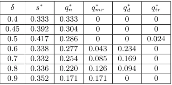
and h∈ {0.04,0.05,0.06}. Table 2.4 is representative of our results.
δ s∗ q∗n q
∗
mr q
∗
d q
∗
ir
0.4 0.333 0.333 0 0 0
0.45 0.392 0.304 0 0 0
0.5 0.417 0.286 0 0 0.024
0.6 0.338 0.277 0.043 0.234 0
0.7 0.332 0.254 0.085 0.169 0
0.8 0.336 0.220 0.126 0.094 0
0.9 0.352 0.171 0.171 0 0
Table 2.4: Equilibrium when the OEM can remanufacture and preemptively collect (β = 1, α= 0.8, h= 0.04)
allows the IR to remanufacture but increases product quality relative to the NR benchmark to undermine the IR’s competitive position. Likewise, whenδ= 0.45, the OEM increases quality relative to the NR benchmark to deter the IR’s entry. The IR is not a competitive threat when
δ≤0.4.
When the remanufactured products’s relative cost-to-value ratio is low, that is, the IR becomes a bigger competitive threat, the OEM uses in-house remanufacturing and preemptive collection jointly to cause scarcity of cores. In particular, whenδ ≥0.6, the OEM remanufac-tures a fraction of the available cores and preemptively collects any remaining cores, deterring the IR’s entry. Furthermore, the OEM remanufactures a larger proportion of collected cores when δ increases indicating a higher perceived value for the remanufactured product. This result is in agreement with our insight from the base model, in which the OEM decreases the production of new product to limit the available cores when the IR becomes a bigger threat.
2.8 Extensions
2.8.1 Price Competition
Here, we study what happens when the OEM and the IR compete in prices. The following proposition describes the equilibrium for the price competition game showing that the structure of the equilibrium is the same as the quantity game.
Proposition 6. The following characterizes the equilibrium regions when the OEM and the IR compete in prices.
R1p. If αδ ≥2, the IR cannot enter the market and the OEM acts like a monopoly.
R2p. If 42+−δδ ≤ α
R3p. If δ(4(10−δ−δ)2) < αδ < 4
−δ
2+δ, the IR enters but does not remanufacture all available cores.
R4p. If 0< αδ ≤ δ(4(10−δ−δ)2), the IR enters the market and remanufactures all available cores.
The equilibrium quality, new and remanufactured product prices and quantities are provided in
the proof of the proposition.
Regions R1p-R4p are the same as regionsR1-R4 of our base model. Specifically, in region
R1p, the IR is not a threat due to its poor cost-to-value position. In region R2p, the OEM chooses a higher quality level compared to the NR benchmark to deter the IR’s entry. In region
R3p, the OEM chooses a higher or lower quality level depending on whether it has the cost-to-value advantage or disadvantage. Finally, in regionR4p, the OEM follows a quantity limiting strategy. Drivers of these results are the same as those in our base model. In region R2p, the OEM’s price is smaller than the monopoly price for its chosen product quality. Different from our base model, the OEM uses price in addition to quality to deter entry in region R2p.
It is well known that price competition is more intense than quantity competition and leads to higher CS and SS (Singh and Vives, 1994). Consistent with this fact, we find that CS and SS are higher than the NR benchmark when the OEM and the IR compete in prices (More detailed analysis of the CS and SS under price competition is relegated to Section A.3). Another artifact of the intense competition is that the new product quantity is always higher than or equal to the NR benchmark. Therefore, remanufacturing by an IR always increases environmental impact under price competition.
2.8.2 Alternative Remanufacturing Cost
Up to this point, we assumed that all remanufacturing related costs are subsumed in βαs2. In this section we consider an additional cost term n that is independent of the quality level. Specifically, the IR’s total unit remanufacturing cost becomes βαs2+n.
We are able to characterize the equilibrium when the OEM has the cost-to-value advan-tage, i.e, αδ ≥ 1, and we state our result in Proposition 7. However, when the IR has the cost-to-value advantage, i.e, αδ < 1, the model is not analytically tractable; therefore we resort to a numerical study. Figure 2.6 demonstrates the results for αδ < 1 as well as for
α
we have run the numerical study for all combinations of δ ∈ {0.2,0.3,0.4,0.5,0.6,0.7,0.9}
andn∈ {0.005,0.010,0.020,0.025,0.030,0.035,0.040,0.045,0.050}and found that they are all consistent. We also study the impact of the quality independent remanufacturing cost on the CS and SS in Appendix A (see Section A.4) and observe numerically that the insights from Propositions 3 and 4 continue to hold.
Proposition 7. The following characterizes the equilibrium regions for αδ ≥ 1 when the IR incurs an additional cost n per unit.
R1i. If αδ ≥ 2, or 2 > αδ > 1 and n ≥ 2δ−α
9β , the IR cannot enter and the OEM acts like a
monopoly.
R2ai. If 2 > αδ ≥ 8−δ
4+δ and
2δ−α
9β > n, or
8−δ
4+δ > α δ ≥
5
4 and
2δ−α
9β > n ≥n0, the IR’s entry is
deterred by the OEM who chooses a quality level higher than the NR benchmark.
R2bi. If 5 4 >
α
δ ≥1 and
2δ−α
9β > n≥n0, the IR’s entry is deterred by the OEM who chooses a
quality level lower than the NR benchmark.
R3i. If 84+−δδ > αδ ≥ 1 and n0 > n, the IR enters the market but does not remanufacture all
available cores.
The equilibrium quality, new and remanufactured product quantities, and n0 are stated in the
proof of the Proposition.
Regions R1i−R3i are same as the regions R1−R3 in the base model. The Proposition demonstrates all three regions that exist in our base model for αδ ≥ 1, namely R1−R3, continue to exist. In addition to these regions an additional region (region R2bi) where the OEM deters the IR’s entry by choosing a quality level lower than the NR benchmark is also possible when the cost-to-value ratio and the quality independent remanufacturing cost are at moderate levels, i.e, −α9+2β δ > n ≥ n0. The OEM’s choice of low quality decreases the
reduction. This allows the OEM to deter the IR’s entry through decreasing quality in the presence of the quality independent cost component. The Proposition also demonstrates that when the quality independent remanufacturing cost is too high, i.e, 2δ−α9β ≤n, the IR cannot enter at all, as expected.
Figures 2.6a and 2.6b illustrate the equilibrium structure for n ∈ 0,0.01,0.02 and n ∈
0.05,0.06 respectively. Figure 2.6a shows that when the IR has a strong cost-to-value position, the OEM may continue to rely on reducing production and limiting core availability (region
R4i). However, as intuition suggests, region R4i gets smaller as n increases. In fact, when
n≥0.02, R4i disappears. Figure 2.6 also shows that as nincreases, the OEM relies more on the quality lever to compete with the IR. However asnincreases, the regions where the OEM chooses a quality level higher than the NR benchmark shrink. In fact, forn≥0.05, the OEM always chooses a lower level of quality (if different from the NR benchmark level).
0 0.1 0.2 0.3 0.4 0.5 0.6 0.7 0.8 0.9 0.24 0.26 0.28 0.3 0.32 0.34 0.36 0.38 0.4 0.42 α Quality R4 (n=0) R3 (n=0) R2a (n=0) R1 (n=0) n=0 n=0.01 n=0.02
(a) n ∈ {0,0.01,0.02} (Partitions R1-R4 are shown for
n= 0)
0 0.1 0.2 0.3 0.4 0.5 0.6 0.7 0.8 0.9 0.22 0.24 0.26 0.28 0.3 0.32 0.34 α Quality R3 (n=0.05) R2b (n=0.05) R1 (n=0.05) n=0.05 n=0.06
(b)n∈ {0.05,0.06}(Partitions R1-R3 are shown forn=
0.05)
Figure 2.6: Equilibrium quality level when the IR incurs quality-independent cost(δ= 0.4, β= 1)
2.8.3 Independent Quality Gap
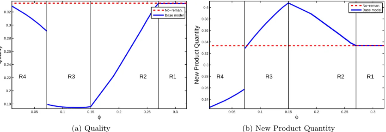
In our base model the quality gap between the new and remanufactured product is proportional to the product quality s. Here, we consider an alternative model in which the quality gap is independent of product quality, specifically the value of remanufactured product is θ(s−φ) for type-θconsumer, where φshows the quality gap for the remanufactured product.
Figure 2.7 shows the equilibrium quality and quantity as quality gapφvaries for α= 0.4. We
find the behavior in this figure to be robust by also checking otherα∈ {0.2,0.3,0.4,0.5,0.6,0.7,0.8,0.9}
values. The Figure identifies four regions similar to our base model (see Proposition 1). In particular, in regionR1, quality gap is sufficiently high and the IR is not a threat. In region
R2, the OEM deters the IR’s entry through its quality choice. In region R3, the quality gap is sufficiently small and the IR remanufactures a portion of available cores. In region R4, the quality gap is very small, and the OEM follows a quantity limiting strategy. This strategy shift is evident in Figure 2.7b as the quantity drops discontinuously between regions R3 and
R4. Note that similar to our base model, when the IR is weak (largeφin this extension), the OEM competes using the quality lever; in contrast when the IR is strong (smallφ), the OEM relies on limiting quantity.
Figure 2.7a demonstrates that the OEM always chooses a lower quality level compared to the NR benchmark. This is the main difference between this extension and our base model. Because the quality gap is independent of the quality level, increasing the quality of the new product also increases the quality of the remanufactured product by the same amount. Therefore, the OEM does not want to increase quality too much which would undermine the relative significance of the quality gap. A lower quality level ensures that the OEM’s quality advantage is sufficiently large relative to the remanufactured product’s perceived quality. When the OEM chooses a much lower quality level than the NR benchmark, this negatively affects social welfare and results in CS and SS levels lower than the NR benchmark (a more detailed analysis is provided in Section A.5).
2.9 Concluding Remarks