Low-cost error mitigation by symmetry verification
X. Bonet-Monroig,1R. Sagastizabal,2,3M. Singh,2,3and T. E. O’Brien1 1Instituut-Lorentz, Universiteit Leiden, P.O. Box 9506, NL-2300 RA Leiden, The Netherlands 2QuTech, Delft University of Technology, P.O. Box 5046, NL-2600 GA Delft, The Netherlands
3Kavli Institute of Nanoscience, Delft University of Technology, P.O. Box 5046, NL-2600 GA Delft, The Netherlands
(Received 9 August 2018; published 28 December 2018)
We investigate the performance of error mitigation via measurement of conserved symmetries on near-term devices. We present two protocols to measure conserved symmetries during the bulk of an experiment, and develop a third, zero-cost, post-processing protocol which is equivalent to a variant of the quantum subspace expansion. We develop methods for inserting global and local symmetries into quantum algorithms, and for adjusting natural symmetries of the problem to boost the mitigation of errors produced by different noise channels. We demonstrate these techniques on two- and four-qubit simulations of the hydrogen molecule (using a classical density-matrix simulator), finding up to an order of magnitude reduction of the error in obtaining the ground-state dissociation curve.
DOI:10.1103/PhysRevA.98.062339
I. INTRODUCTION
Noisy, intermediate scale quantum (NISQ) devices have begun to appear in laboratories around the world. These devices have performance rates around or just below the quantum error correction threshold [1–5], but are lacking the number of qubits required for full fault-tolerant quantum computing. This raises the open question of whether the upcoming generation of quantum computers will provide a quantum advantage over classical computers, and in which fields this might be achieved [6–8]. In particular, for the area of digital quantum simulation, it has been suggested that variational quantum eigensolvers [9] may be sufficiently low cost to be performed on ∼50 qubits [10–13]. Around this point, solving the many-body problem exactly becomes too challenging for classical computers, and a slight quantum edge might be available above current approximations.
In lieu of full error correction techniques, much atten-tion is being turned to error mitigaatten-tion techniques, which, although unscalable, promise modest improvements at low cost. Previous work has focused on active error minimization, whereby data is obtained at artificially increased error rates and then extrapolated to zero [14–17], and on probabilistic error cancellation, where an ensemble of noisy circuits is applied such that they average to the target error-free circuit [14,18]. More specific techniques have been developed for quantum simulation, and in particular for variational quantum eigensolvers. A technique developed for exploring the low-energy excited subspace of a quantum system, the quantum subspace expansion, has been shown to have error mitigation as a side effect [19,20].
In this work we investigate error mitigation via verification of symmetries found in quantum circuits, in particular those in physical systems. This is a low-cost version of the stabilizer parity checks ubiquitous in quantum error correction [21,22]. We develop multiple protocols to perform symmetry verifi-cation, both repeatedly throughout a quantum circuit and as
a single post-processing step. The latter can be related to a variant of the quantum subspace expansion [19]. We study the sensitivity of symmetry verification to different noise channels, and demonstrate how it can be optimized by adding new symmetries and rotating existing symmetries to be more sensitive to local noise.
II. DEFINITIONS
In this section we cover some basic definitions to be used throughout this paper, and some details of quantum computing that may be skipped by the experienced reader. We use the Pauli group onNqubitsPN= {I, X, Y, Z}⊗Nthroughout this
work. These operators form a basis for operators ˆO∈C2N
,
ˆ
O=
ˆ
P∈PN
OPˆP ,ˆ (1)
with coefficientsOPˆ inC. If we chooseOPˆ ∈R, this is then a basis for the 2N×2N Hermitian matrices. We call such a
basis decomposition of an operator ˆOa Pauli decomposition. Such a basis is orthogonal in the Frobenius norm:
||Oˆ||F =
Tr[ ˆO†Oˆ]. (2)
Elements ˆP ∈PN have two eigenvalues p= ±1, with
cor-responding eigenspaces of dimension 2N−1, and projectors ˆ
Mp =12(1+pP) onto said eigenspaces. The Pauli group has
an additional property; if ˆP =I⊗N ∈PN, ˆP commutes with
half of the elements ofPN ([ ˆP ,Qˆ]=0), and anticommutes
with the other elements ({P ,ˆ Rˆ} =0). This property can be extended to a general operator ˆO—[ ˆP ,Oˆ]=0 ({P ,ˆ Oˆ} =0) if and only if ˆP commutes (anticommutes) with each element of the Pauli decomposition of ˆO[Eq. (1)].
represented as a vector|φin the complex vector spaceC2N. Transformation consists of evolving this state to a new state
|ψ ∈C2N
, which may be represented via a unitary opera-tor |ψ =U|φ (with U∈U(C2N),i.e., U U†=U†U =I). Measurement consists of observing the quantum state |ψ
along some degree of freedom. The degree of freedom is represented by a projector-valued measurement{Mˆi}for each
possible observed value i, where iMˆi =I, ˆMi2=Mˆi†=
ˆ
Mi. The observation records one such valueiat random with
probabilitypifollowing the Born rule,
pi = |ψ|Mˆ|ψ|2, (3)
and the state of the system collapses into ˆMi|ψ/pi.
In the presence of noise, the state of a qubit is instead given by a density matrix ρ ∈DN, where DN is the set of
2N×2N positive, trace 1 matrices. These are a generalized
form of pure quantum states|ψ, which allow for statistical ensembles of pure states (the well-known adage being that preparing √1
2(|0 + |1) is strictly not the same as preparing
|0or|1with 50% probability). For every pure state|ψ, the corresponding density matrix is the outer product|ψψ|, and the expectation value of an operator ˆOmay be calculated as
ψ|Oˆ|ψ =Tr[ ˆO|ψψ|]. (4) We will use the latter notation throughout this paper, to be consistent with calculating expectation values on mixed states ρ (where the standard bra-ket expectation value is no longer possible). We will distinguish between operators ˆO
and density matricesρby the use of hats. Note that the trace of products of density matrices is also well defined, and has an obvious interpretation as the overlap between the density matrices, as for pure states,
Tr[|ψψ||φφ|]= ψ|φφ|ψ = |φ|ψ|2. (5)
Transformations and measurements of density matrices be-have differently to those of pure states [23], but we will not need details of this in this work.
A quantum algorithm incurs a cost based on the number of qubits and coherence time required for quantum hard-ware to execute it. This cost is usually increased by error mitigation protocols that require additional gates or ancilla qubits. However, these are in general low cost compared to the overhead required for full quantum error correction. Indeed, some error mitigation protocols require no additional quantum hardware or circuitry, hence we define them as “zero cost.” Such protocols may require repetition of the algorithm in order to estimate expectation values Tr[ ˆOρ], but this may be offset by parallelizing across multiple quantum devices. This cost metric is then similar to the quantum volume [7] often used to characterize quantum hardware.
III. SYMMETRY VERIFICATION
Our study is motivated by the presence of symmetries in quantum mechanical systems. In such systems, one has a Hamiltonian ˆH, and is usually interested in studying the properties of ground or low-lying eigenstates of the system. A (unitary) symmetry of a system is a unitary operator ˆSthat commutes with the Hamiltonian—[ ˆH ,Sˆ]=0. When this is
true, ˆH may be block diagonalized within the eigenspaces of ˆ
S. Then, if one were to study eigenstates of ˆH on a quantum computer, one may perform such a study entirely within a single target eigenspace S of ˆS. In real-world quantum computers, noise may shift the state of the computer outside of the target eigenspaceS. By verifying during or at the end of a calculation that the system remains inS, and throwing away results where this is not the case, it is thus possible to make our quantum computation less sensitive to these types of noise.
Verification of a symmetry is performed by measurement and post-selection which is typically performed in the com-putational basis (the eigenstates|0and|1of a single qubit). The Pauli operators PN may be rotated into this basis
rela-tively easily (see Sec.IV), and as such are a good class from which to draw symmetry operators. If ˆS /∈PN, but the target
eigenspaceSlies within the eigenspace of a Pauli operator ˆP, then measuring ˆP presents a low-cost alternative to measuring
ˆ
S, though this may provide less error mitigation in the case where the eigenspace of ˆP is strictly larger thanS. In general, symmetry verification will work with any construction of a projector valued measurement{Mˆi}where one projector ˆMS
projects onto the target eigenspace S. We note that phase estimation [24] provides a generic construction for such a measurement, although this is a rather high cost circuit (in particular requiring the ability to apply the symmetry ˆU on the quantum computer). This requirement for measurement implies that symmetry verification cannot be extended to antiunitary symmetries (nor to symmetries that anticommute with the Hamiltonian), as these do not lead to eigenspaces that can be projected into.
The projector valued measurement{Mˆi}is the more
gen-eral object for symmetry verification than the symmetry ˆS. In an arbitrary quantum circuit at an arbitrary time, if we know by any means that the state|ψin the absence of error satisfies ˆMs|ψ = |ψ, measuring{Mˆi}on the noisy state ρ
and post-selecting will project to the state,
ρs =
ˆ
MsρMˆs
Tr[ ˆMsρ]
. (6)
Then, we have
Tr[ρs|ψψ|]=
Tr[ρ|ψψ|] Tr[ ˆMsρ]
Tr[ρ|ψψ|], (7)
and our new stateρshas strictly greater overlap with the target |ψ than the pre-selection ρ (unless ˆMsρMˆs=ρ, in which
caseρs=ρ). Such a procedure can be immediately extended
to multiple operators ˆS1,Sˆ2, . . ., as long as [ ˆSi,Sˆj]=0. (If
this is not the case, sequential symmetry verification projects between different eigenspaces, which is inefficient and greatly increases the number of experiments that must be thrown away.) Symmetry verification may also be repeated at multiple points during a quantum circuit, by inserting measurement of
ˆ
FIG. 1. Quantum circuit for ancilla symmetry verification of a symmetry ˆS. (a) A simple circuit entangling all qubits with a single ancilla qubit. The rotations ˆRidepend on the tensor components ˆSi
on each qubiti (relationship given in text). (b) A circuit making an identical measurement to that in (a), but with only local CNOT
andSWAPtwo-qubit gates. ASWAPbetween qubit 0 and the ancilla is not required because the Bell state prepared after the firstCNOT
is symmetric between the two qubits (this is not the case for the remaining qubits).
IV. ANCILLA AND IN-LINE SYMMETRY VERIFICATION
The simplest form of the symmetry verification involves the use of an ancilla qubit to measure the Pauli symmetry ˆS. Let us write ˆS∈Pnin terms of its tensor factors; ˆS= ⊗iSˆi,
and let NS be the number of nontrivial ˆSi= {X, Y, Z}. To
each such ˆSi, we can associate a corresponding rotation ˆRi = {exp(iπ
2Y),exp(−i
π
2X),1}(such that ˆRi|Sˆi =1 = |0). The verification circuit is then shown in Fig.1(a). For each nontriv-ial ˆSi, the corresponding qubit is rotated by ˆRi, then performs
a controlled-NOT gate on the ancilla qubit, and finally is rotated by ˆR−i1. This requires that the ancilla qubit be coupled to each qubit in the system register that it measures, which is in general not possible in a quantum circuit. As a low-cost alternative [Fig.1(b)], the ancilla qubit may be shuffled along the system register viaSWAPgates as it performs the controlled phase gate. In either case, as the ancilla qubit must interact with each register qubit individually, the circuit depth must be
O(NS).
It is possible to forego the ancilla qubit in symmetry verification, by instead encrypting the symmetry ˆS onto the computational degree of freedom of a qubit within the system itself, which is then read out. In Fig. 2(a) we give an ex-ample circuit for this in-line symmetry verification, with cir-cuit depth onlyO(log(NS)). This logarithmic depth requires
qubits to be coupled as a binary tree, which is not possible in systems which allow only local couplings. In general, for such ad-dimensional local coupling, the depth of the circuit must be at leastO(NS1/d), being the minimum depth of a light-cone encompassingNSqubits. In Fig.2(b)we give such a circuit
for a system with linear connectivity. Even when all-to-all coupling is available, theO(log(NS))-depth circuit [Fig.2(a)]
FIG. 2. Quantum circuits for in-line symmetry verification. (a) The optimal verification circuit hasO(log(NS)) depth, but requires
long-range connectivity between qubits, which is not available on many architectures. (b) In the presence of linear connectivity, an O(NS) depth verification circuit is optimal.
may not be preferable, as the duty cycle for each qubit (i.e., the period of time between the first and last gate each qubit is involved in) is length O(log(NS)). By contrast, the duty
cycle of an individual qubit during the circuit in Fig.1(b)is
O(1). A short duty cycle implies that qubits can be used to perform other operations while the symmetry verification is ongoing, reducing the time cost when this circuit is performed as a small block of a larger computation.
V. VARIATIONAL QUANTUM EIGENSOLVERS
As an example target algorithm for symmetry verification, we consider ground-state preparation for a Hamiltonian ˆH
via a variational quantum eigensolver [9,25]. An (ideal) varia-tional quantum eigensolver consists of a unitary circuitU(θ), parametrized by a vector of free anglesθthat control individ-ual gates within the circuit. This circuit acts on a starting state, which we take to be the computational basis state|0, . . . ,0, to produce a variational final state |ψ(θ) =U(θ)|0, . . . ,0. These angles are controlled classically to minimize the energy
E(θ)= ψ(θ)|Hˆ|ψ(θ). This expectation value is calculated in an experiment by taking the Pauli decomposition of ˆH
[Eq. (1)], preparing|ψ(θ)and measuring each ˆPi repeatedly
to accumulate statistics onψ|Pˆi|ψ.
Jordan-Wigner transformation on an N-fermion Hamiltonian, this symmetry takes the formZ⊗N. Most VQEs consist of creating
an approximate starting state (such as the Hartree-Fock state) that respects this symmetry, and then performing multiple local rotations that continue to respect this symmetry. This is true of both the unitary coupled cluster (UCC) ansatz [9], and the quantum approximate optimization algorithm (QAOA) [26]. In the former, the ansatz is taken as the expansion of the cluster operatoreTˆ−Tˆ†,
ˆ
T =
n
ˆ
T(n), (8)
ˆ
T(n)=
i1,...,in;j1,...,jn
θi1,...,in
j1,...,jn n
m=1 ˆ
c†i
m
n
m=1 ˆ
cjm
, (9)
where theθparameters are taken as the free parameters to be optimized, and the sum is a sum over empty molecular orbitals to the left of the semicolon, and filled molecular orbitals to the right. This exponentiation is typically performed by the Trotter-Suzuki expansion, leaving a series of unitaries,
i;j
eθji( ˆc †
icˆj−cˆ†jcˆi)
i,j;k,l
eθk,li,j( ˆc † icˆ
† jcˆkcˆl−cˆ†lcˆ
†
kcˆjcˆi). . . , (10)
each of which respects fermion parity. QAOA for the elec-tronic structure problem consists of performing steps of time evolution alternating between the Hartree-Fock Hamiltonian and the electronic-structure Hamiltonian, both of which re-spect fermion parity. Thus, for both ansatz, bulk symmetry verification could be performed between individual steps of the time evolution.
Although symmetry verification promises a final state with greater overlap with the ground state, it does not promise a necessarily lower energy. Let us write the (un-normalized) symmetry-accepted stateρs, and the symmetry-rejected state
ρr. If our measurement was perfect, we would have
ρs =MˆsρMˆs, ρr=(I−Mˆs)ρ(I−Mˆs). (11)
Then, Tr[ ˆH ρ]=Tr[ ˆH ρr]+Tr[ ˆH ρs]. Now, suppose the
re-jected state ρr has lower energy than the accepted stateρs;
Tr[ ˆH ρr]
Tr[ρr]
< Tr[ ˆH ρs]
Tr[ρs]
. (12)
We can calculate
Tr[ ˆH ρ]=Tr[ρr]
Tr[ ˆH ρr]
Tr[ρr] +
Tr[ρs]
Tr[ ˆH ρs]
Tr[ρs]
<(Tr[ρr]+Tr[ρs])
Tr[ ˆH ρs]
Tr[ρs] =
Tr[ ˆH ρs]
Tr[ρs]
,
and our symmetry-verified state would be higher in energy than the initial state as well. As the energy ofρr lies strictly
above the ground state, failure of symmetry verification must implyρshas sufficiently large overlap with high-energy states.
As such, we would suggest that such a failure implies the energy ofρitself is not to be trusted.
VI. POST-SELECTED SYMMETRY VERIFICATION AND S-QSE
Conveniently, when a quantum computation requires cal-culating the expectation values of a set of Pauli operators, symmetry verification may be performed via post-processing of the expectation values themselves (with possibly some additional measurements), rather than requiring additional quantum circuitry. Suppose we want to calculate the expecta-tion value of ˆP ∈PNon our stateρfollowing projection onto
the ˆS=s(= ±1) subspace of our symmetry ˆS∈PN. The projector onto this subspace may be written ˆMs =12(1+sSˆ).
Then, the expectation value of ˆP on the state ρs targeted by
the symmetry verification can be expanded using Eq. (6),
Tr[ ˆP ρs]=Tr
ˆ
P MˆsρMˆs
Tr[ ˆMsρ]
=Tr[ ˆP ρ]+sTr[ ˆPSρˆ ]
1+sTr[ ˆSρ] , (13)
where we have used the cyclic property of the trace and the fact that [ ˆP ,Mˆs]=0 to write Tr[ ˆPMˆsρMˆs]=Tr[ ˆPMˆsρ],
and expanded our definition of ˆMs. The expectation values
Tr[ ˆSρ], Tr[ ˆP ρ], and Tr[ ˆPSρˆ ] may be then calculated using the unverified stateρ, and substituted into Eq. (13) to obtain the verified result. By avoiding additional quantum circuitry, we expect this method to outperform both ancilla and in-line symmetry verification. However, we note that post-selection cannot be used for bulk symmetry verification (as we cannot measure these expectation values during the circuit). Further-more, it cannot be used in algorithms where the output is not an expectation value Tr[ ˆP ρ].
Post-selected symmetry verification can be observed to be identical to a form of the quantum subspace expansion (QSE) [19]. Originally designed to investigate the low-energy excited states around the ground space found by a variational quantum eigensolver, QSE works by taking a set of excitation operators
{Eˆi}, which can be applied to the approximated ground state |ψ(θ)to obtain a set of states|φi =Eˆi|ψ(θ). The spectrum
of the Hamiltonian within the manifold spanned by these states can be calculated as the solution to the generalized eigenvalue problem,
ˆ
HQSE|ξ =λBˆQSE|ξ. (14)
Here, HˆQSE is the Hamiltonian matrix projected into the spanned manifold,
[ ˆHQSE]i,j =Tr[ ˆH|φiφj|], (15)
and ˆBQSEis the overlap matrix,
[ ˆBQSE]i,j =Tr[|φiφj|], (16)
to account for the fact that |φi and |φj are in general not
orthogonal. In the presence of noise, although the state |φi
is not well defined (as our noisy stateρ is not a pure state), the operators|φiφj| =EˆiρEˆj†remain well defined, and the
expectation values in Eqs. (15) and (16) are still able to be measured in an experiment.
The set {Eˆi}is usually taken to be the set of low-order
if the set{I,Sˆ}is chosen as excitation operators, the solution to the generalized eigenvalue problem is the same as that obtained by post-selection. To show this, we expand
Tr[ ˆH ρs]=
i
hiTr[ ˆPiρs]
=
i
Tr[hiPˆiρ]+sTr[hiPˆiSρˆ ]
1+sTr[ ˆSρ]
=Tr[ ˆH ρ]+sTr[ ˆHSρˆ ]
1+sTr[ ˆSρ] . (17) Next, we calculate the QSE matrices (using the commutation of ˆHand ˆS),
ˆ
HQSE=
Tr[ ˆHρ] Tr[ ˆHSρˆ ]
Tr[ ˆHSρˆ ] Tr[ ˆH ρ] , (18)
ˆ
BQSE=
1 Tr[ ˆSρ]
Tr[ ˆSρ] 1 . (19)
Assuming that Tr[ ˆSρ]=1, ˆBQSE is invertible, the problem reduces to finding the (regular) eigenvalues of
ˆ
BQSE−1 HˆQSE= 1 1−Tr[ ˆSρ]2
α β β α
, (20)
where
α=Tr[ ˆH ρ]−Tr[ ˆSρ]Tr[ ˆHSρˆ ], (21)
β=Tr[ ˆHSρˆ ]−Tr[ ˆH ρ]Tr[ ˆSρ]. (22)
The eigenvalues of this matrix take the form,
λ= 1
1−Tr[ ˆSρ]2(α±β) (23)
= Tr[ ˆH ρ]±Tr[ ˆHSρˆ ]
1±Tr[ ˆSρ] , (24) which can be seen to be equal to those found in Eq. (17). We call this version of the quantum subspace expansion symmetry-QSE, or S-QSE for short.
This result is not surprising; it was suggested in [19] to account for symmetries during QSE by projecting ˆHQSE and
ˆ
BQSE into the symmetry subspace, which achieves the same result as in the above. However, this demonstrates that one may account for symmetries via a version of QSE without calculating the full linear response. Moreover, this implies that S-QSE corrects for both coherent and incoherent errors that project out of the ˆS=s subspace. By contrast, QSE with an operator that anticommutes with the Hamiltonian can only correct coherent errors (see Appendix). S-QSE may be immediately combined with other forms of QSE, for example, linear response QSE, by including both sets of operators as excitations.
VII. SIMULATION OF SYMMETRY VERIFICATION ON THE HYDROGEN MOLECULE
To first investigate symmetry verification in a simple set-ting, we use a VQE to find the ground-state energy of H2
on two qubits. This follows previous experimental demon-strations [9,20,27,28]. We take the STO-3G basis for H2, which has four spin orbitals, and convert this into a qubit Hamiltonian via the Bravyi-Kitaev transformation. The four spin orbitals require four qubits to represent them on, but in this representation the Hamiltonian is diagonal on two of the qubits, which may be removed. The remaining two-qubit Hamiltonian takes the form,
ˆ
H =h0II+h1IZ+h2ZI+h3XX+h4Y Y+h5ZZ,
(25)
where hi are sums of integrated two- and four-body terms
from the original electronic structure problem. The calculation of these terms, and the Bravyi-Kitaev transformation itself, were performed using the PSI4 [29] andOPENFERMION [30] packages. The Hamiltonian can be seen to commute with the symmetry ˆS=ZZ. Our ground-state wave function has nontrivial overlap with the Hartree-Fock wave function, which is in theZZ= −1 subspace; this is then our target subspace. We follow the unitary coupled cluster ansatz of [27], which consists of exciting our system to the|01state, and perform-ing the unitary rotation,
ˆ
U(θ)=e−iθ X0Y1. (26)
This unitary rotation may be decomposed using standard methods [31]. As described previously, the VQE procedure consists of fixing θ, repeatedly preparing|ψ(θ) and mea-suring collections of terms in the Pauli decomposition of ˆH
until a good estimate of the energyE(θ) is found. This is then repeated at varying θ as demanded by a classical optimizer until a minimumE(θ) is found [9].
We compare the performance of the three symmetry ver-ification protocols described previously as a final symmetry verification step. The ancilla symmetry verification is per-formed in the same manner as Fig.1(a). The in-line symmetry verification is performed in a manner similar to Fig.2(a), but as this is final symmetry verification, we have no need to undo the symmetry measurement. Instead, to measure the expecta-tion value of a Pauli operator Tr[ρPˆ], we can propagate ˆP
through the symmetry verification circuit [32] and measure the corresponding Pauli term. It is then sufficient to rotate the control qubit to recover the expectation values IZand
XX. From this we may calculate all other expectation values in Eq. (25) using the fact that ZZ= −1. For this problem, S-QSE not only requires no additional circuitry, but also no additional measurements (all required terms are in the Pauli decomposition of the Hamiltonian).
To test symmetry verification in the presence of realistic noise, we simulate our chosen experiment using the quantum-sim density matrix quantum-simulator [33]. We take gate error models and parameters similar to previous simulation work based on experimental data of state-of-the-art superconducting trans-mon qubits [34]. Errors in transmon qubits are dominated by decoherence times, which we take at a base level to beT1=
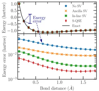
FIG. 3. Accuracy of the VQE over the entire bond dissociation curve using the different symmetry verification methods mentioned in the text (labeled in legend). (Top) The target curve of H2,
com-pared to the exact result (black line). (Bottom) Log plot of the difference between the black lines and points in the above plot.
verification purposes) has a read-out error of 1%, and that error in tomographic measurements and pre-rotations (used to calculate the expectation values themselves) can be canceled by linear inversion tomography [35,36].
Using the above error model, we observe (Fig.3) that the unmitigated VQE (blue points) achieves an error in the energy of approximately 0.01–0.04 hartree across the bond dissoci-ation curve. This error is improved upon by all symmetry verification techniques. S-QSE (red diamonds) provides the largest improvement of all symmetry verification protocols, as no additional errors are introduced. The S-QSE circuit is observed to give approximately a fivefold improvement over the unmitigated circuit, while ancilla (orange crosses) and in-line (green squares) symmetry verification show an ap-proximately twofold and threefold improvement, respectively. The differences between S-QSE and other forms of symmetry verification emphasize the importance of minimizing the ver-ification cost in bulk symmetry verver-ification (where S-QSE is no longer available).
We now investigate the effect of different noise channels on the performance of symmetry verification. Any noise channel that commutes with the symmetry operators evolves the system state within the target subspace, which symmetry verification explicitly does not mitigate. The analysis of which channels have this property can be reduced to an analysis over PN, as if we mitigate Pauli errors ˆP
i∈PN, we also mitigate
any linear combination of them [21]. In the above circuit, theZZ symmetry commutes with any single-qubitZerrors, making the protocol prone to theTφ(pure dephasing) channel,
but it anticommutes with single-qubit X errors, making the protocol resilient against theT1(amplitude decay) channel. To investigate this, in Fig.4we calculate the error in determining the ground-state energy near the minima of the bond dissocia-tion curve (0.75 Å bond distance) using S-QSE, as we varyT1 andTφ. We turn all other error sources off, and varyT1 (Tφ)
withTφ =20μs (T1 =20μs) fixed. In the absence of error
10
010
110
210
3T
1,
T
φ(
μ
s)
10
−310
−210
−1Energy
error
(hartree)
ErrorTφ= 20μs Error S-QSETφ= 20μs ErrorT1= 20μs
Error S-QSET1= 20μs
FIG. 4. Effect of varying decoherence times on the VQE ac-curacy. With all other error sources turned off, T1 is varied with
Tφ=20μs fixed (red-dashed curves), andTφ is varied withT1=
20μs fixed (blue-solid curves). We plot the error in estimating the ground-state energy for the unmitigated experiment (squares), and the circuit mitigated with S-QSE (circles). Data points for the blue and red curves are identical atT1=Tφ=20μs, as can be seen from
the complete overlap.
mitigation, the two decoherence sources have almost identical effect (deviation approximately 10−2hartree). However, in the presence of error mitigation, the susceptibility of the VQE to
T1noise is noticeably smaller than toTφnoise—up to a factor
of two over the range of decoherence times plotted. We note that S-QSE does not make our circuit second-order sensitive toT1noise. This can be understood asXerrors at some points during our VQE circuit are rotated toZerrors by later gates in the circuit, preventing their mitigation.
VIII. INSERTING AND ROTATING SYMMETRIES
As observed in the previous section, verifying single sym-metries has a marked effect on the performance of a quantum circuit, but will not catch and remove all sources of noise. In this section we suggest how one may improve upon this by adding additional symmetries to the quantum algorithm, and by rotating existing symmetries to make them more sensitive to errors on the underlying quantum hardware. In the language of quantum error correction, this is a low-cost attempt to increase the distance of the detection code.
We first suggest a method to extend anN-qubit Hamilto-nian ˆH, given a Pauli operator ˆP ∈PN, to an N+1-qubit
Hamiltonian ˆHext,
ˆ
Hext=
ˆ
H 0
0 PˆHˆPˆ
. (27)
Both blocks of ˆHextcan be seen to have the same eigenspec-trum (as this is unaffected by the unitary rotation of ˆP), and
ˆ
Hextcommutes with the operator,
0 Pˆ
ˆ
P 0
=XP ,ˆ (28)
which is then the new symmetry operator. This mapping cor-responds to mapping Pauli operators ˆQ∈PN in the original
problem to
ˆ
Qext=
IQˆ if [ ˆQ,Pˆ]=0
To implement this in the algorithm itself, we note that every circuit can be decomposed into a product of unitary rotations,
j
eiθjQˆj Qˆ
j ∈PN, (30)
where a single ˆQ∈PN may be repeated in the product.
Adding the symmetry then consists of replacing these ro-tations by roro-tations around the transformed operator ˆQext
[as per Eq. (29)], and re-decomposing the operations into a circuit (using, e.g., the methods of [31,37]). If ˆH had a previous set of symmetries ˆSi, these are transformed to a new
set ˆSi,ext [following Eq. (29)], that commute with both ˆHext and the additional symmetryXPˆ. This extension method is particularly suitable for digital quantum simulation, as circuits are often generated in the form of Eq. (30). This is the case for traditional Hamiltonian simulation [38], quantum phase estimation [31], and the UCC QSE discussed previously, all of which require exponentiating an operator via the Suzuki-Trotter expansion [39].
Beyond choosing the number of symmetries in a problem, one may wish to choose how these symmetries appear in the problem. In particular, sets of symmetries may be found that anticommute with all local operators, which should increase the mitigation power of the verification protocol against local sources of noise. (For example, theN-qubit operators X⊗N
andZ⊗N with evenN.) Any two groups ofMPauli operators are unitarily equivalent as long as they satisfy the same com-mutation and multiplication rules (e.g.,IZ,ZI, andZZ are equivalent toXX,Y Y, andZZ, but not toIX,IY, andIZ). To find such unitary transformations, we suggest decomposing them into rotations of the form ˆR=eiπ2Qˆ for ˆQ∈P, which
transforms
ˆ
P ∈P→Rˆ†PˆRˆ =
ˆ
P if [ ˆP ,Qˆ]=0
iPˆQˆ if{P ,ˆ Qˆ} =0. (31)
Rotations of this form have a few desirable properties. Their effect is easy to calculate classically, and they transform Pauli operators to Pauli operators. Furthermore, each ˆRleaves half of the Pauli group unchanged. This allows for some choice of rotations to leave desired symmetries (or other operators) already present in the problem invariant, while other terms are rotated.
IX. EXTENDING THE SYMMETRY VERIFICATION OF THE HYDROGEN MOLECULE
We now demonstrate the verification of multiple symme-tries by extending the previous VQE simulation of H2. We transform the electronic structure Hamiltonian onto a qubit representation this time via the Jordan-Wigner transformation. This gives the four-qubit Hamiltonian,
ˆ
H=hII+
i
hiZi+
1 2
i=j
hi,jZiZj +hs(X0Y1Y2X3
+Y0X1X2Y3−X0X1Y2Y3−Y0Y1X2X3), (32)
which has symmetries ˆS0=Z0Z1, ˆS1=Z0Z2, and ˆS2=
Z0Z1Z2Z3. In the Bravyi-Kitaev transformation these sym-metries were the additional qubits that were thrown away. We
FIG. 5. Adding and adjusting symmetries to optimize symmetry verification. The blue (dots) and red (diamonds) curves correspond to their colored (shaped) counterparts in Fig. 3, while the purple (squares) and brown (crosses) curves come from a four-qubit simula-tion of H2using the two protocols described in the text. The dashed
lines represent the S-QSE versions of their solid counterparts. Error parameters on all qubits are the same for all simulations (parameters given in the text).
choose again the unitary coupled cluster ansatz for the VQE, which can be reduced to the operator [40],
ˆ
U(θ)=eiθ Y0X1X2X3. (33)
As in the two-qubit case, the VQE circuit consists of preparing the system in the Hartree-Fock state |1100, applyingU(θ) and measuring the variational energy, for a total circuit time of 400 ns.
The above set of symmetries still commute with all single-qubit Z errors, so we rotate our problem to increase the mitigation power of symmetry verification. We choose the rotation,
ˆ
R =eiπ2Y0X2eiπ2Y1X3. (34)
This transforms the symmetry ˆS0→X0X1X2X3, while leav-ing ˆS1 and ˆS2 unchanged. The resulting set of symmetries do not commute with any single-qubit X or Z operator, as required. To create the transformed circuit, we need to transform both our starting state|1100 →Rˆ|1100, and the UCC unitary ansatz,
ˆ
U(θ)→RˆUˆRˆ†=eiθ Y0Z1X2. (35)
The transformed circuit incurs an additional cost from this initial application of ˆR, but this is balanced by the reduced weight of the transformed cluster operator, resulting in a total circuit time of 440 ns.
studied, this simulation achieves a twofold reduction in error compared to the two-qubit S-QSE simulation, despite using twice as many qubits and a twice as long circuit. By compar-ison, unrotated S-QSE on four qubits cannot protect against the T2 noise accumulated over the simulation, and performs a factor of two worse than the two-qubit S-QSE simulation. This clearly demonstrates the need to optimize symmetry verification protocols to account for errors present in the system as this technique is scaled up to larger computations. Over the entire bond-dissociation curve, the rotated four-qubit S-QSE simulation outperforms its unmitigated counterpart by over an order of magnitude.
X. CONCLUSION
In this paper we have presented a low-cost strategy for error mitigation, which we call symmetry verification. We have discussed various ways in which it can be applied to different algorithms, and various methods to optimize the mitigation power against common sources of error. We have demonstrated these protocols on a simulated VQE experiment of H2, and observed that they outperform the unmitigated result over the entire bond-dissociation curve by around an order of magnitude.
Although the above techniques are very promising for small experiments, much work needs to be done optimizing symmetry verification for midrange experiments in the NISQ era. The addition and choice of symmetries needs to be inves-tigated further to minimize the resulting circuit depth. Further study is also needed on the optimal number of symmetry verifications to be added to a circuit, both to maximize mitiga-tion and minimize run time (which increases exponentially in the number of verifications made). Finally, given the obvious connection between symmetry verification and the stabilizer formalism of quantum error correction, it is natural to ask whether one can mix the two to transform slowly between midsize NISQ circuits and large-scale fault-tolerant ones.
While this paper was in production, a related work by McArdle et al. [41] appeared on the ArXiv. They simulate the performance of ancilla symmetry verification for a VQE, and its combination with other error mitigation strategies to further improve robustness against noise. Their results are consistent with and complementary to our own, and they provide useful techniques for measuring non-Pauli operators not considered in this work.
ACKNOWLEDGMENTS
The authors wish to thank Carlo Beenakker, Leonardo DiCarlo, Brian Tarasinski, Barbara Terhal, Detlef Hohl, Luuk Visscher, Francesco Buda, Yaroslav Herasymenko, and Adriaan Rol for feedback, advice, and support in this project. This research was supported by the Netherlands Organization for Scientific Research (NWO/OCW) and by an ERC Synergy Grant.
APPENDIX: ERROR MITIGATION OF QSE WITH ANTICOMMUTING OPERATORS
In this appendix we repeat the analysis of QSE from the text, but with an operator ˆA that anticommutes with the
Hamiltonian ˆH. Let us assume to begin that ˆA is unitary. Such an operator cannot be simultaneously diagonalized with
ˆ
H, and so we have no result from symmetry verification to compare with. Given an eigenstate ˆH|ψ =E|ψ, we have that ˆHAˆ|ψ = −AˆHˆ|ψ = −EAˆ|ψ, and so the presence of an anticommuting operator splits the eigenstates of ˆH into pairs of equal magnitude but opposite sign energies (known as eigenstates of different chirality). If ˆA=Aˆ†, the eigenstates of
ˆ
Aitself are the equal superpositions,
|± = √1
2(|ψ ± ˆ
A|ψ). (A1)
For QSE, we must calculate the operators ˆHQSEand ˆBQSE.
ˆ
BQSE=
1 Tr[ ˆAρ]
Tr[ ˆA†ρ] 1 . (A2)
ˆ
HQSE=
Tr[ ˆHρ] Tr[ ˆHAρˆ ]
Tr[−HˆAˆ†ρ] −Tr[ ˆH ρ] . (A3)
Again assuming |Tr[ ˆAρ]|2=1, we can invert ˆBQSE and calculate
ˆ
BQSE−1 HˆQSE= 1
1− |Tr[ ˆAρ]|2
α β
−β∗ −α∗ , (A4)
where
α=Tr[ ˆH ρ]+Tr[ ˆAρ]Tr[ ˆHAρˆ ], (A5)
β=Tr[ ˆHAρˆ ]+Tr[ ˆH ρ]Tr[ ˆAρ]. (A6)
The solution to the equation is
EQSE2 = |α|
2+ |β|2
(1− |Tr[ ˆAρ]|2)2 (A7)
= Tr[ ˆH ρ]2+ |Tr[ ˆHAρˆ ]|2
1− |Tr[ ˆAρ]|2 . (A8)
To understand the gain in energy, |Tr[ ˆHAρˆ ]|2, let us first consider a single set of opposite chirality states|ψand ˆA|ψ
(with energy ±E). We first note that if ρ is an incoherent superposition of the eigenstates,
ρ= |a|2|ψψ| + |b|2Aˆ|ψψ|A,ˆ (A9)
Tr[ ˆHAρˆ ]=Tr[ ˆAρ]=0 (asψ|A|ψ =0), and QSE strictly does not improve on the estimate of the ground-state energy. We next consider the opposite situation, whereρis a coherent superposition of eigenstates:
ρ =(cos(θ)|ψ +sin(θ)eiφAˆ|ψ)
×(cos(θ)ψ| +sin(θ)e−iφψ|Aˆ†). (A10) We can calculate
Tr[ ˆH ρ]=Ecos(2θ), (A11)
Tr[ ˆAρ]=sin(2θ)(1+Aeiφ), (A12)
whereA= ψ|Aˆ2|ψ(so|A|1, and for ˆA∈PN,A=1). This gives
EQSE2 =E2cos
2(2θ)+sin2(2θ)χ
+
1−sin2(2θ)χ− , (A14) χ±=(1±Aeiφ)(1±Ae−iφ). (A15)
We see that ifA=1, φ= π
2, QSE corrects the coherent error entirely, while ifA=1, φ=0 it has no effect. This implies that QSE cannot correct coherent rotations of ρ from |ψ
towards an eigenstate of ˆA. This is in keeping with the general observations in [19] for the performance of QSE as an error mitigation strategy.
If ˆAis not unitary, then ˆA†Aˆ is a Hermitian operator that commutes with ˆH. Importantly, if{A,ˆ Hˆ} =0,{AˆH ,ˆ Hˆ} =0 as well, giving a second anticommuting operator that is in gen-eral nonunitary. This could be used directly in QSE, although the analysis of Sec.VIno longer holds unless ˆA†Aˆ ∈P2. For symmetry verification, we require the form of the projector
ˆ
Ma onto the correct ˆA†Aˆ|ψ =a|ψ subspace. This is a
difficult task in general to construct (for ˆAHˆ, it is equivalent to diagonalizing the Hamiltonian). We have been unable to construct any further bounds on the performance of QSE as an error mitigation strategy for a general Hermitian operator, nor for an operator which neither commutes nor anticommutes with ˆH. This is, however, an interesting direction for future research.
[1] D. Ristè, S. Poletto, M.-Z. Huang, A. Bruno, V. Vesterinen, O.-P. Saira, and L. DiCarlo,Nat. Commun.6,6983(2015). [2] R. Barends, J. Kelly, A. Megrant, A. Veitia, D. Sank, E. Jeffrey,
T. C. White, J. Mutus, A. G. Fowler, B. Campbell, Y. Chen, Z. Chen, B. Chiaro, A. Dunsworth, C. Neill, P. O’Malley, P. Roushan, A. Vainsencher, J. Wenner, A. N. Korotkov, A. N. Cleland, and J. M. Martinis,Nature (London)508,500(2014). [3] S. Debnath, N. M. Linke, C. Figgatt, K. A. Landsman, K.
Wright, and C. Monroe,Nature536,63(2016).
[4] T. Monz, D. Nigg, E. A. Martinez, M. F. Brandl, P. Schindler, R. Rines, S. X. Wang, I. L. Chuang, and R. Blatt,Science351, 1068(2016).
[5] N. Ofek, A. Petrenko, R. Heeres, P. Reinhold, Z. Leghtas, B. Vlastakis, Y. Liu, L. Frunzio, S. M. Girvin, L. Jiang, M. Mirrahimi, M. H. Devoret, and R. J. Schoelkopf,Nature (Lon-don)536,441(2016).
[6] J. Preskill,Quantum2,79(2018).
[7] N. Moll, P. Barkoutsos, L. S. Bishop, J. M. Chow, A. Cross, D. J. Egger, S. Silipp, A. Fuhrer, J. M. Gambetta, M. Ganzhorn, A. Kandala, A. Mezzacapo, P. Müller, W. Riess, G. Salis, J. Smolin, I. Tavernelli, and K. Temme, Quantum Science and Technology3,030503(2018).
[8] C. Neill, P. Roushan, K. Kechedzhi, S. Boixo, S. V. Isakov, V. Smelyanskiy, A. Megrant, B. Chiaro, A. Dunsworth, K. Arya, R. Barends, B. Burkett, Y. Chen, Z. Chen, A. Fowler, B. Foxen, M. Giustina, R. Graff, E. Jeffrey, T. Huang, J. Kelly, P. Klimov, E. Lucero, J. Mutus, M. Neeley, C. Quintana, D. Sank, A. Vainsencher, J. Wenner, T. C. White, H. Neven, and J. M. Martinis,Science360,195(2018).
[9] A. Peruzzo, J. McClean, P. Shadbolt, M.-H. Yung, X.-Q. Zhou, P. Love, A. Aspuru-Guzik, and J. O’Brien,Nat. Commun.5, 4213(2014).
[10] R. Babbush, N. Wiebe, J. McClean, J. McClain, H. Neven, and Garnet Kin-Lic Chan,Phys. Rev. X8,011044(2018). [11] D. Poulin, A. Kitaev, D. S. Steiger, M. B. Hastings, and M.
Troyer,Phys. Rev. Lett.121,010501(2018).
[12] D. W. Berry, M. Kieferová, A. Scherer, Y. R. Sanders, G. H. Low, N. Wiebe, C. Gidney, and R. Babbush,npj Quant. Inf.4, 22(2018).
[13] I. D. Kivlichan, J. McClean, N. Wiebe, C. Gidney, A. Aspuru-Guzik, Garnet Kin-Lic Chan, and R. Babbush,Phys. Rev. Lett.
120,110501(2018).
[14] K. Temme, S. Bravyi, and J. M. Gambetta,Phys. Rev. Lett.119, 180509(2017).
[15] Y. Li and S. C. Benjamin,Phys. Rev. X7,021050(2017). [16] A. Kandala, K. Temme, A. D. Corcoles, A. Mezzacapo, J. M.
Chow, and J. M. Gambetta,arXiv:1805.04492. [17] M. Otten and S. Gray,arXiv:1806.07860.
[18] S. Endo, S. C. Benjamin, and Y. Li,Phys. Rev. X8, 031027 (2018).
[19] J. R. McClean, M. E. Kimchi-Schwartz, J. Carter, and W. A. de Jong,Phys. Rev. A95,042308(2017).
[20] J. I. Colless, V. V. Ramasesh, D. Dahlen, M. S. Blok, M. E. Kimchi-Schwartz, J. R. McClean, J. Carter, W. A. de Jong, and I. Siddiqi,Phys. Rev. X8,011021(2018).
[21] D. Gottesman,arXiv:0904.2557.
[22] B. M. Terhal,Rev. Mod. Phys.87,307(2015).
[23] M. A. Nielsen and I. L. Chuang,Quantum Computation and Quantum Information, Cambridge Series on Information and the Natural Sciences (Cambridge University Press, Cambridge, 2000).
[24] A. Y. Kitaev,arXiv:quant-ph/9511026.
[25] J. R. McClean, J. Romero, R. Babbush, and A. Aspuru-Guzik, New J. Phys.18,023023(2016).
[26] E. Farhi, J. Goldstone, and S. Gutmann,arXiv:1411.4028. [27] P. J. J. O’Malley, R. Babbush, I. D. Kivlichan, J. Romero, J.
R. McClean, R. Barends, J. Kelly, P. Roushan, A. Tranter, N. Ding, B. Campbell, Y. Chen, Z. Chen, B. Chiaro, A. Dunsworth, A. G. Fowler, E. Jeffrey, E. Lucero, A. Megrant, J. Y. Mutus, M. Neeley, C. Neill, C. Quintana, D. Sank, A. Vainsencher, J. Wenner, T. C. White, P. V. Coveney, P. J. Love, H. Neven, A. Aspuru-Guzik, and J. M. Martinis,Phys. Rev. X6,031007 (2016).
[28] A. Kandala, A. Mezzacapo, K. Temme, M. Takita, M. Brink, J. M. Chow, and J. M. Gambetta,Nature (London)549, 242 (2017).
[30] J. R. McClean, I. D. Kivlichan, K. J. Sung, D. S. Steiger, Y. Cao, C. Dai, E. Schuyler Fried, C. Gidney, B. Gimby, P. Gokhale, T. Häner, T. Hardikar, V. Havlíˇcek, C. Huang, J. Izaac, Z. Jiang, X. Liu, M. Neeley, T. O’Brien, I. Ozfidan, M. D. Radin, J. Romero, N. Rubin, N. P. D. Sawaya, K. Setia, S. Sim, M. Steudtner, Q. Sun, W. Sun, F. Zhang, and R. Babbush,arXiv:1710.07629. [31] J. D. Whitfield, J. Biamonte, and A. Aspuru-Guzik,Mol. Phys.
109,735(2011).
[32] D. Gottesman,Group22: Proceedings of the XXII International Colloquium on Group Theoretical Methods in Physics, edited by S. P. Corney, R. Delbourgo, and P. D. Jarvis (International Press, Cambridge, MA, 1999), pp. 32–43.
[33] The QUANTUMSIM density matrix simulator can be found at https://github.com/quantumsim/.
[34] T. E. O’Brien, B. Tarasinski, and L. DiCarlo,npj Quant. Inf.3, 39(2017).
[35] S. Filipp, P. Maurer, P. J. Leek, M. Baur, R. Bianchetti, J. M. Fink, M. Göppl, L. Steffen, J. M. Gambetta, A. Blais, and A. Wallraff,Phys. Rev. Lett.102,200402(2009).
[36] J. M. Chow, L. DiCarlo, J. M. Gambetta, A. Nunnenkamp, L. S. Bishop, L. Frunzio, M. H. Devoret, S. M. Girvin, and
R. J. Schoelkopf, Phys. Rev. A 81, 062325
(2010).
[37] M. B. Hastings, D. Wecker, B. Bauer, and M. Troyer, Quant. Inf. Comput.15, 1 (2015).
[38] I. M. Georgescu, S. Ashhab, and F. Nori,Rev. Mod. Phys.86, 153(2014).
[39] M. Suzuki,Comm. Math. Phys.51,183(1976).
[40] The cluster operator for this system is a sum of eight four-qubit terms, however, the action of each term on the Hartree-Fock starting state is identical, so only one is needed.