| INVESTIGATION
A Powerful Variant-Set Association Test Based on
Chi-Square Distribution
Zhongxue Chen,*,1Tong Lin,†and Kai Wang‡
*Department of Epidemiology and Biostatistics, School of Public Health, Indiana University Bloomington, Indiana 47405,†The Key Laboratory of Machine Perception (Ministry of Education), School of EECS, Peking University, Beijing 100871, China, and
‡Department of Biostatistics, College of Public Health, University of Iowa, Iowa 52242
ABSTRACTDetecting the association between a set of variants and a given phenotype has attracted a large amount of attention in the scientific community, although it is a difficult task. Recently, several related statistical approaches have been proposed in the literature; powerful statistical tests are still highly desired and yet to be developed in this area. In this paper, we propose a powerful test that combines information from each individual single nucleotide polymorphism (SNP) based on principal component analysis without relying on the eigenvalues associated with the principal components. We compare the proposed approach with some popular tests through a simulation study and real data applications. Our results show that, in general, the new test is more powerful than its competitors considered in this study; the gain in detecting power can be substantial in many situations.
KEYWORDSchi-square distribution; gene-set analysis; principal component analysis
W
ITH the innovations of biomedical and biochemicaltechnologies, large amounts of genetic sequencing data have been produced, providing researchers with great opportu-nities to investigate the genetic contributions to some phenotypes such as cancers. Genome-wide association studies (GWASs) have successfully identified thousands of single nucleotide poly-morphisms (SNPs) that are associated with some common
diseases (Manolio et al. 2009; Chen and Ng 2012; Chen
2013; Chenet al. 2017b). However, most of those identified SNPs from GWAS are variants with relatively high minor allele
frequencies (MAFs). Rare variants (e.g., SNPs with MAF,5%)
may play a critical role in disease development (Bodmer and Bonilla 2008). Nevertheless, because of their low MAFs, rare variants are usually removed from data analysis in GWASs. And, even if they were included, current statistical methods designed for GWASs may have very limited power to detect the signal if the sample sizes are not large enough. Instead of testing a single variant a time, researchers have proposed statistical approaches to detecting the possible association between a
set of variants and a phenotype. Recently, many statistical methods have been designed specifically for gene-set or path-way rare-variant data analysis (Li and Leal 2008; Madsen and Browning 2009; Han and Pan 2010; Basu and Pan 2011; Lin
and Tang 2011; Wuet al.2011, 2015; Yi and Zhi 2011; Lee
et al.2012; Shaet al.2012; Panet al.2014; Wang 2016; Chen et al.2017a; Chen and Wang 2017).
The sequencing kernel association test (SKAT) is among the most popular rare-variant association testing methods. The SKAT is essentially based on the principal component analysis (PCA). More specifically, it calculates a test statistic from each individual principal component of the covariance matrix of the genotype data, and then takes the weighted sum of these statistics as the overall test statistic, where the weights are the associated eigen-values. The null distribution of the overall test statistic is a linear combination of chi-square distributions, which can be approxi-mated by a chi-square distribution (Davies 1980; Liuet al.2009), from which aP-value can be approximated.
The optimal sequencing kernel association test (SKAT-O) is a weighted sum of the SKAT and a burden test, which assumes the directions are the same and the magnitudes are similar among all of the rare variants under study (Leeet al.2012). Therefore, the SKAT-O in general is more robust than the SKAT. However, like the SKAT, the SKAT-O still uses the information from eigenvalues. In addition, both the SKAT and the SKAT-O require assigning weigh to each variant (e.g., a function of MAF).
Copyright © 2017 by the Genetics Society of America doi:https://doi.org/10.1534/genetics.117.300287
Manuscript received May 4, 2017; accepted for publication September 10, 2017; published Early Online September 13, 2017.
Supplemental material is available online atwww.genetics.org/lookup/suppl/doi:10. 1534/genetics.117.300287/-/DC1.
The use of the eigenvalues as weights in the SKAT can be
beneficial if indeed the major principal components have
stronger association with the phenotype. However, if this assumption is not met, the SKAT can potentially lose power dramatically. In addition, assigning weights to variants can be challenging. To circumvent these difficulties, in this paper, we propose a new statistical association testing method for rare-variant data analysis. This new test has some nice properties, such as simple form and computational efficiency. To study the performance of the proposed approach, we compare it with some popular methods. Our comparison results show that the new test is more powerful than the SKAT and SKAT-O tests under most of the situations studied. Real data applications are also given to illustrate the use of the new approach.
Methods
We use y¼ ðy1;y2;⋯;ynÞ9 to denote phenotypes (either qualitative or quantitative) of the nsubjects in a study. As-sumeXn3p are the observations ofpcovariates fromn sub-jects, andGn3k are thekgenotypes fromnsubjects, where the (i,j) component ofGn3k;gi;j¼0;1;or 2 if the number of copies of the minor allele of the jth SNP from the ith subject is zero, one, or two, respectively. Denote the standardized re-siduals (i.e., the raw residual divided by its estimated SD) z¼ ðz1;z2;⋯;znÞ9of y after adjusting for the p covariates using a generalized linear model (e.g., a logistic regression model for binary phenotype and ordinary linear regression for conditions phenotype). Then, to detect the association
between the set of the kSNPs and the phenotype, we can
conduct an overall test betweenzand the genotypes. Letl1$l2$⋯$ln$0 be theneigenvalues of matrix
GWWG9 ;whereG is the centeredG(i.e., each component is subtracted by its column mean),W¼diagðw1;w2;⋯;wkÞis the weight matrix, andui¼ ðui1;ui2;⋯;uinÞ9the eigenvector associated withli(i¼1;2;. . .;n). By default, the SKAT uses wi¼dbetaðMAFi;1;25Þ; where dbetað;a;bÞ is the density function of abetadistribution with the two shape parameters a and b;and MAFiis the MAF of the ith SNP, which can be estimated from the data. Unless otherwise specified, in this paper, we use the default weighting function for both of the SKAT and the SKAT-O tests.
The SKAT statistic is asymptotically equivalent to the following expression (Wuet al.2011):
SKAT¼z9GWW G9z ¼X
n
i¼1 li
z9ui
2
ð1Þ:
It is easy to see that, under the null hypothesis, none of thek SNPs is associated with the phenotype, SKAT asymptotically follows a linear combination of chi-square distributions,
Pn
i¼1
lix2i;1;wherex2i;1are independently and identically
distrib-uted (iid)x2
1distribution with degree of freedom (df) 1. Alternatively, the test statistic SKAT can be rewritten as:
SKAT¼li
z9vi
2
ð2Þ;
whereliis the ith nonzero eigenvalue ofWG9 GW ;viis the ith column of matrixGW UD ;Dis ak3kdiagonal matrix with Dii¼li21=2ifli6¼0;0 otherwise; andU is the eigenvectors matrix ofWG9 GW :It can be shown that the eigenvectorui associated with nonzero eigenvalueliofGWW G9 can be cal-culated as the correspondingvidefined above. In fact, letui be the eigenvector associated with eigenvalueliofG9 G W ði¼1;2;⋯;kÞ; then WG9 GW ui¼liui: The above defined vi can be rewritten as vi¼GW ui=
ffiffiffiffi li
p
for li6¼0: Then,
GWWG9v i¼GWW G9ffiffiffiGWui li
p ¼liGWffiffiffiui
li
p ¼livi: This shows thatvi is
the eigenvector associated with nonzero eigenvalue li:Use the fact that the two sets of nonzero eigenvalues from con-formable matricesAB(e.g.,GWW G9) and BA(e.g.,WG9 GW) are the same, the set of nonzero eigenvalues offligare the same as {li}. Therefore, bothfvig are fuig are the sets of eigenvectors associated with nonzero eigenvalues ofGWW G’; and the equations in (1) and (2) are equivalent. However, ex-pression (2) is preferred whenkis smaller thann, as the com-putation is more efficient in this situation. From (2), the asymptotic null distribution of SKAT is a linear combination of
chi-square distributions,P k
i¼1
lix2i;1:
From either (1) or (2), we can see that the SKAT is actually a weighted chi-square test with weights equal to the associated eigenvalues. Therefore, the SKAT is sensitive to the eigenvalues;
Table 1 Empirical type I error rate (31=a) for each method using significance levels a¼1024;1025;and 106replicates when there
are 5, 10, 20, 50, and 100 SNPs with 1000 cases and 1000 controls
r Test
#SNP
5 10 20 50 100
0 SKAT 1.04 1.07 0.89 0.86 1.00
1.1 1.5 0.7 0.4 1.2
SKATO 1.10 1.13 0.74 1.05 0.94
1.0 1.6 0.5 0.8 1.1
Burden 0.98 1.15 0.84 1.30 0.98
0.8 0.9 0.5 1.4 0.7
C 1.08 1.27 0.86 1.15 0.88
1.1 1.9 0.8 0.6 0.7
0.2 SKAT 1.0 1.21 0.98 0.64 0.85
1.5 1.3 1.4 0.6 1.0
SKATO 0.87 1.14 0.94 0.60 1.00
1.3 1.3 1.2 0.8 1.2
Burden 0.96 1.29 1.05 0.73 1.13
0.9 1.5 1.1 0.8 1.0
C 1.18 1.04 1.12 0.65 0.84
1.3 0.9 0.9 0.5 0.9
20.2 SKAT 0.98 1.02 0.88 1.06 0.70
1.8 1.0 0.7 1.3 0.8
SKATO 1.08 1.03 0.92 1.26 0.72
1.4 1.0 1.0 1.3 0.8
Burden 1.15 0.96 0.95 1.03 1.00
1.5 0.8 1.3 1.0 0.8
C 1.03 0.95 0.80 0.95 0.86
its performance largely depends on how strong the major principal components correlate withzcompared with other principal com-ponents. In the cases where the correlations betweenzand the major principal components are not stronger than those betweenz and other principal components, the SKAT may perform poorly. Motived by this observation, we propose a robust test without using eigenvalues. We useCto denote the new test statistic that has the following expression.
C¼X
k
i¼1
z9vi
2
ð3Þ:
It can be shown that the above new test has the following properties.
Theorem 1
Under the null hypothesis, C asymptotically follows a
chi-square distribution withdf¼k9;wherek9is the number of nonzero eigenvalues ofWG9GW :
Proof:Without loss of generality, we assumek¼k9:It is easy to
show that under the null hypothesis, asymptotically,z9vifollows a normal distribution with mean 0 and variance 1, and the covariance between z9vi and z9vj (i6¼j) is 0. Therefore, ðz9viÞ2 ði¼1;2;. . .;kÞ is asymptotically independently and identically distributed as ax2
1:
Theorem 2
Cis invariant of the weightW:
Proof: Supposeui ði¼1;2;⋯;kÞare thekeigenvectors of
G9G; denote U¼ ½u1u2⋯uk; then we have U9G9 GU ¼ L¼diagðl1;l2;⋯;lkÞ;whereUU9¼I; and Iis the identity
matrix. In addition, we have WG9GW ¼VL1V9; where
L1¼diagðlð11Þ;l
ð1Þ
2 ;⋯;l
ð1Þ
k Þ and VV9¼I; then U9WG9
GWU¼U9VL1V9U¼ ðU9VÞL1ðU9VÞ9:SinceðU9VÞ ðU9VÞ9¼ U9VV9U’¼I;each column of matrixU9Vis also the eigenvectors
of matrix WG9 GW : Therefore, from (3), C¼P k
i¼1
ðz9viÞ2¼z9
ðPk i¼1
vivi9Þz¼z9ð
Pk i¼1
uiV9Vui9Þz¼z9ð
Pk i¼1
uiui9Þz:
According to Theorem 2, we can calculate the statisticC without assigning weight to each SNP.
In the next section, we will compare the proposed test with the SKAT and the optimal SKAT (SKAT-O) through a simula-tion study.
Data availability
Supplemental Material, File S1contains Supplemental
Ta-bles based on simulation study and real data application.File S2is the R code of the proposed test.
Results
Simulation study
Simulation settings:In the simulation study, we mainly focus
on comparing the proposed test (C) with the sequencing ker-nel association test (SKAT), the optimal sequencing kerker-nel
Table 2 Empirical type I error rate (31=a) for each method using significance levels a¼1024;1025; and 106replicates when there
are 5, 10, 20, 50, and 100 SNPs with 2000 subjects and continuous phenotypes
r Test
#SNP
5 10 20 50 100
0 SKAT 1.12 1.00 0.90 1.00 1.12
0.8 1.1 1.1 1.3 1.1
SKATO 0.98 1.09 0.93 1.01 1.09
1.0 1.7 0.9 1.2 1.00
Burden 0.85 1.00 1.11 1.05 1.35
0.8 0.7 1.3 0.7 1.3
C 0.97 1.01 0.78 1.06 0.93
0.6 1.0 0.9 0.8 1.2
0.2 SKAT 1.02 1.18 0.95 0.96 0.92
1.1 1.3 0.7 1.5 1.1
SKATO 1.02 0.82 1.15 0.96 0.92
1.1 0.6 1.0 1.1 0.5
Burden 0.94 1.00 1.03 1.01 0.93
1.1 0.9 0.7 0.9 0.8
C 0.88 1.22 0.93 1.00 0.98
0.6 1.2 1.2 0.9 0.9
20.2 SKAT 0.85 1.08 1.03 1.04 0.99
1.1 1.0 0.7 1.8 1.3
SKATO 0.80 0.93 0.89 1.06 1.02
0.3 1.1 0.4 0.8 0.5
Burden 1.22 0.93 0.97 1.14 0.78
1.2 0.9 1.8 0.1 0.6
C 1.02 0.98 1.07 0.82 1.17
0.9 1.1 1.2 0.7 1.1
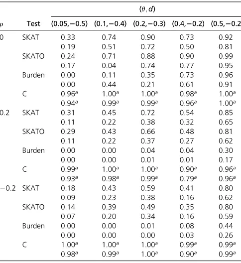
Table 3 Empirical power of each method using significance levels a¼1024and 1025when there are 1000 cases, 1000 controls and
100 SNPs with 10% of those 100ucausal SNPs are protective
r Test
(u;d)
(0.05,20.5) (0.1,20.4) (0.2,20.3) (0.4,20.2) (0.5,20.2)
0 SKAT 0.33 0.74 0.90 0.73 0.92
0.19 0.51 0.72 0.50 0.81
SKATO 0.24 0.71 0.88 0.90 0.99
0.17 0.04 0.74 0.77 0.95
Burden 0.00 0.11 0.35 0.73 0.96
0.00 0.44 0.21 0.61 0.91
C 0.96a 1.00a 1.00a 0.98a 1.00a
0.94a 0.99a 0.99a 0.96a 1.00a
0.2 SKAT 0.31 0.45 0.72 0.54 0.85
0.11 0.22 0.38 0.32 0.65
SKATO 0.29 0.43 0.66 0.48 0.81
0.11 0.22 0.37 0.27 0.62
Burden 0.00 0.00 0.04 0.04 0.30
0.00 0.00 0.01 0.01 0.17
C 0.99a 1.00a 1.00a 0.90a 0.96a
0.93a 0.98a 0.99a 0.79a 0.96a
20.2 SKAT 0.18 0.43 0.59 0.41 0.80
0.09 0.23 0.38 0.16 0.62
SKATO 0.14 0.39 0.49 0.35 0.80
0.07 0.20 0.34 0.16 0.59
Burden 0.00 0.00 0.01 0.08 0.44
0.00 0.00 0.00 0.03 0.26
C 1.00a 1.00a 1.00a 0.99a 0.99a
association test (SKAT-O), and the burden test. We use the
program, simRareSNP (http://www.biostat.umn.edu/weip/),
provided by W. Pan to generate case-control rare-variant SNP data. For the genotype data, we use a latent multivariate Gauss-ian variable with compound symmetry (CS) as their covarGauss-iance structure. The correlation coefficient (r) in the CS takes different values,e.g.,r¼0; 0:2;20:2;in the simulation study. We sim-ulate SNPs with MAFs ranging from 0.001 to 0.05.
To investigate how the new method controlling type I error rate, we simulate 50 and 100 null SNPs, 1000 cases, and 1000 controls. Using significance level 1024and 1025, we obtain the empirical type I error rate based on 106 repli-cates. We also consider using 700 cases and 1300 controls.
To estimate the power value, we randomly select a
pro-portion (u) of 100 variants as causal SNPs, where utakes
values 0.05, 0.1, 0.2, 0.4, and 0.5. Following the simulation settings as described in the SKAT paper, we assume the effect size of each causal SNP is a function of MAF. Specifically, we assume the magnitude of logarithmic relative risk (RR) of
het-erozygous to homozygous major genotypes isd3log10ðMAFÞ;
with various values for d; 20:2;20:3; 20:4; and20:5: The logarithmic RR is very close to the logarithmic odds ratio (OR), which was used with similar magnitudes for simulation study in the SKAT paper, if the disease prevalence is low. Of those causal SNPs, we randomly assign 10, 50, and 90% as protective variants, and the rest are risk variants. The commonly used log-additive genetic model is assumed in the simulation. The genotype frequencies of cases can be determined by those of controls and the relative risks of heterozygous and
homozygous minor to homozygous major (Chen et al.
2012, 2014a, 2016a; Chen and Ng 2012; Chen 2014). Spe-cifically, if the genotype frequencies of homozygous minor,
heterozygous, and homozygous major are p0, p1and p2(q0,
q1, and q2), respectively, for controls (cases), and the relative risks of heterozygous and homozygous minor to homozygous major are r1and r2, then we have the following relationships.
8 > > > > > > > > < > > > > > > > > :
q0¼
p0
p0þr1p1þr2p2
q1¼
r1p1
p0þr1p1þr2p2
q2¼
r2p2
p0þr1p1þr2p2
ð4Þ:
We then consider continuous phenotypes. We use the same procedure as described above to generate genotype data for 2000 subjects. For phenotype, we randomly select a
por-tion (u) of SNPs as casual variants with 10, 50, and 90%
of them having positive effects. The effect for the jth causal SNP is set asbj¼signðbjÞ3d3log10ðMAFjÞ;wheresignðbjÞ takes 1 (21) with probability 0.1 (0.9), 0.5 (0.5), and 0.9
(0.1), and d takes different values 20.25, 20.2, 20.15,
and 20.1 (i.e., half of the d values for the above case-control situations). For the ith subject, the phenotype is
yi¼
Pk
j¼1
bjgijþei;wheregijis the genotype (0, 1, or 2) andei
are independently and identically distributed as the standard normal distribution.
Table 4 Empirical power of each method using significance levels a¼1024and 1025when there are 1000 cases, 1000 controls and
100 SNPs with 50% of those 100ucausal SNPs are protective
r Test
(u;d)
(0.05,20.5) (0.1,20.4) (0.2,20.3) (0.4,20.2) (0.5,20.2)
0 SKAT 0.43 0.75 0.86 0.77 0.91
0.27 0.59 0.71 0.47 0.81 SKATO 0.33 0.66 0.80 0.59 0.85 0.24 0.48 0.55 0.35 0.72 Burden 0.00 0.00 0.01 0.00 0.02 0.00 0.00 0.00 0.00 0.01 C 0.83a 0.98a 0.99a 0.97a 1.00a
0.76a 0.90a 0.99a 0.95a 0.99a
0.2 SKAT 0.17 0.47 0.71 0.56 0.87 0.05 0.23 0.41 0.43 0.72 SKATO 0.15 0.44 0.68 0.51 0.83 0.05 0.22 0.41 0.38 0.66 Burden 0.00 0.00 0.00 0.00 0.00 0.00 0.00 0.00 0.00 0.00 C 0.79a 0.99a 1.00a 0.97a 1.00a
0.70a 0.93a 0.99a 0.90a 0.99a
20.2 SKAT 0.22 0.45 0.59 0.49 0.77 0.10 0.26 0.38 0.28 0.48 SKATO 0.19 0.38 0.54 0.39 0.71 0.09 0.21 0.30 0.19 0.38 Burden 0.00 0.00 0.00 0.00 0.00 0.00 0.00 0.00 0.00 0.00 C 0.97a 1.00a 1.00a 0.99a 1.00a
0.87a 0.99a 0.98a 0.96a 1.00a aThe highest power value for each comparison
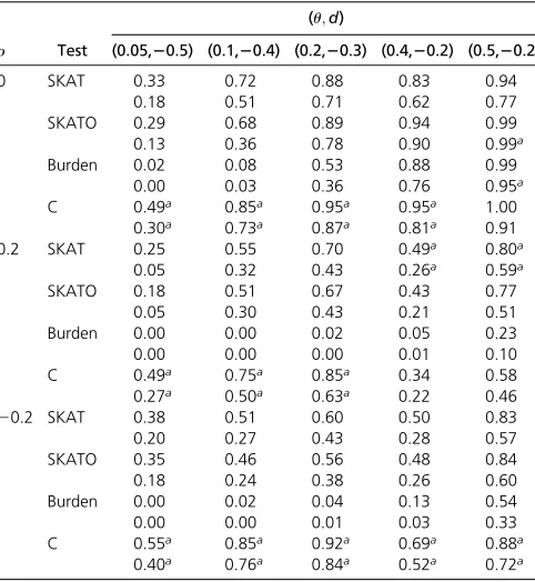
Table 5 Empirical power of each method using significance levels a¼1024and 1025when there are 1000 cases, 1000 controls and
100 SNPs with 90% of those 100ucausal SNPs are protective
r Test
(u;d)
(0.05,20.5) (0.1,20.4) (0.2,20.3) (0.4,20.2) (0.5,20.2)
0 SKAT 0.33 0.72 0.88 0.83 0.94
0.18 0.51 0.71 0.62 0.77
SKATO 0.29 0.68 0.89 0.94 0.99 0.13 0.36 0.78 0.90 0.99a
Burden 0.02 0.08 0.53 0.88 0.99 0.00 0.03 0.36 0.76 0.95a C 0.49a 0.85a 0.95a 0.95a 1.00
0.30a 0.73a 0.87a 0.81a 0.91
0.2 SKAT 0.25 0.55 0.70 0.49a 0.80a
0.05 0.32 0.43 0.26a 0.59a
SKATO 0.18 0.51 0.67 0.43 0.77
0.05 0.30 0.43 0.21 0.51
Burden 0.00 0.00 0.02 0.05 0.23
0.00 0.00 0.00 0.01 0.10
C 0.49a 0.75a 0.85a 0.34 0.58
0.27a 0.50a 0.63a 0.22 0.46
20.2 SKAT 0.38 0.51 0.60 0.50 0.83
0.20 0.27 0.43 0.28 0.57
SKATO 0.35 0.46 0.56 0.48 0.84
0.18 0.24 0.38 0.26 0.60
Burden 0.00 0.02 0.04 0.13 0.54
0.00 0.00 0.01 0.03 0.33
C 0.55a 0.85a 0.92a 0.69a 0.88a
Simulation results: Table 1 reports the relative empirical type I error rates (empirical rate to the preset type I error rate) for all methods included in the comparison. It shows that under various conditions, all methods controlled type I error rate well. Table 3, Table 4, and Table 5 give the empir-ical power values (the highest power value is highlighted for each comparison) from each test when 1000 cases and 1000 controls were simulated, with the proportion of pro-tective causal variants being 10, 50, and 90%, respectively. We observe the following patterns. First, when the SNPs are
independent (i.e., r¼0), all methods have higher power
values compared with the situations when the SNPs are not independent (i.e.,r¼0:2; or 20:2). Second, as expected,
when u (the proportion of causal variants) increases while
dfixed (e.g.,d¼ 20:2 andu¼0:4 and 0:5), the power in-creases for each method. Third, for most of the conditions, the proposed test has the largest empirical power values. In addi-tion, the power gain of the new test over the SKAT and the SKAT-O tests are substantial under many scenarios.
For the situations where the phenotypes are simulated as continuous variables, Table 2 reports the type I error rate for each method. It shows that all of the methods can control type I error rate well. Table 6, Table 7, and Table 8 give the empirical power values for each method under various conditions. From the simulation results, we have similar observations as those from the case-control situations. As suggested by one reviewer, we also considered many other situations, including (1) differ-ent numbers of cases and controls, (2) various number of SNPs,
(3) keep d the same value while letuvary, (4) effect sizes are independent of MAF, and (5) all SNPs have the same MAF value. The simulation results can be found from File S1 . In general, we observed similar patterns as those from Table 1, Table 3, Table 4, Table 5, Table 6, Table 7, and Table 8.
Real Data Applications
In this section, first, we use the Genetic Analysis Workshop 17 (GAW17) data to demonstrate the application of the proposed method. The GAW17 uses the information of a subset of genes with sequencing data available in the 1000 Genomes Project. In
GAW17, SNPs from gene ELAVL4 influence the simulated
quan-titative phenotype Q1; and gene VNN1 is associated with the simulated quantitative phenotype Q2. Except for the genetic risk factors, both Q1 and Q2 were also assumed to be associated with some covariates, such as age, gender, and smoking status. For each gene, the phenotype (Q1 or Q2 values) was simulated 200 times in the GAW17 data set; therefore, 200P-values can be obtained by each method. We use a linear regression model to account for the effects of those nongenetic factors first, then applied our proposed test, along with SKAT, SKAT-O, and the burden test, to the standardized residuals obtained from the regression.
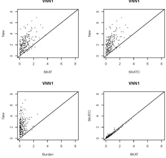
Figure 1 and Figure 2 plot the2log10(P-values) obtained by those methods from genes ELAVL4 and VNN1, respec-tively. These plots clearly show that the proposed test
pro-duced smallerP-values compared to SKAT, SKAT-O, and the
burden test, for most cases. This indicates that the proposed
Table 6 Empirical power of each method using significance levels a¼1024and 1025when there are 2000 subjects with continuous
phenotypes and 100 SNPs with 10% of those 100ucausal SNPs having positive effects
r Test
(u;d)
(0.05,20.25) (0.1,2020 (0.2,20.15) (0.4,20.10) (0.5,20.10)
0 SKAT 0.54 0.76 0.81 0.84 0.93
0.33 0.50 0.69 0.63 0.80
SKATO 0.42 0.69 0.85 0.93 1.00
0.23 0.45 0.71 0.88 0.99
Burden 0.01 0.08 0.37 0.79 0.98
0.01 0.01 0.23 0.65 0.95
C 0.81a 0.98a 0.99a 1.00a 1.00
0.62a 0.97a 0.95a 0.93a 0.99
0.2 SKAT 0.81 0.98 1.00 1.00 1.00
0.67 0.95 0.99 1.00 1.00
SKATO 0.81 0.98 1.00 1.00 1.00
0.67 0.95 0.99 1.00 1.00
Burden 0.54 0.88 0.98 1.00 1.00
0.41 0.86 0.98 1.00 1.00
C 0.88a 1.00a 1.00 1.00 1.00
0.75a 0.98a 1.00 1.00 1.00
20.2 SKAT 0.74 0.93 0.99 1.00 1.00
0.62 0.91 0.99 1.00 1.00
SKATO 0.76 0.94 0.99 1.00 1.00
0.64 0.91 0.99 1.00 1.00
Burden 0.47 0.82 0.98 1.00 1.00
0.34 0.76 0.98 1.00 1.00
C 0.97a 1.00a 1.00a 1.00 1.00
0.89a 0.99a 1.00a 1.00 1.00 aThe highest power value for each comparison
Table 7 Empirical power of each method using significance levels a¼1024and 1025when there are 2000 subjects with continuous
phenotypes and 100 SNPs with 50% of those 100ucausal SNPs having positive effects
r Test
(u;d)
(0.05,20.25) (0.1,2020 (0.2,20.15) (0.4,20.10) (0.5,20.10)
0 SKAT 0.45 0.77 0.85 0.80 0.90
0.31 0.61 0.70 0.61 0.79
SKATO 0.44 0.68 0.76 0.69 0.87
0.26 0.55 0.56 0.44 0.73
Burden 0.00 0.01 0.00 0.01 0.00
0.00 0.01 0.00 0.00 0.00
C 0.85a 0.98a 1.00a 0.95a 1.00a
0.74a 0.92a 0.96a 0.92a 0.99a
0.2 SKAT 0.39 0.63 0.82 0.69 0.83
0.20 0.33 0.52 0.50 0.62
SKATO 0.37 0.60 0.78 0.65 0.83
0.20 0.33 0.52 0.49 0.61
Burden 0.11 0.15 0.22 0.15 0.15
0.07 0.11 0.14 0.06 0.11
C 0.79a 0.90a 1.00a 0.98a 1.00a
0.58a 0.83a 0.99a 0.94a 0.98a
20.2 SKAT 0.40 0.52 0.67 0.56 0.75
0.29 0.38 0.46 0.35 0.58
SKATO 0.36 0.51 0.64 0.51 0.71
0.26 0.36 0.44 0.28 0.56
Burden 0.06 0.16 0.11 0.08 0.10
0.03 0.07 0.06 0.05 0.06
C 0.90a 0.96a 1.00a 0.99a 1.00a
test is more powerful than its competitors. For some situa-tions, the improvements of the new method were substantial.
We then applied the new method, along with others, to the ocular hypertension treatment study (OHTS) data (Gordon and Kass 1999). OHTS is a National Eye Institute-sponsored multi-center, randomized clinical trial. Its goal is to investi-gate the efficacy of medical treatment in delaying or prevent-ing the onset of primary open angle glaucoma (POAG) in individuals with elevated intraocular pressure. This data set includes 249 non-Hispanic Black individuals between 40 and 80 years old were enrolled and genotyped in a subsequent study. Data for this genetic study is available at Database of Genotypes and Phenotypes (dbGaP, Study Accession phs000240.v1.p1). There were 1,051,295 genotyped SNPs. The HGNC gene symbols were obtained using the R/Biocon-ductor package biomaRt (version 2.26.1). There are 30,562 autosomal genes. Genes that contain more than two SNPs were excluded from further consideration.
In this application, we want to detect the association between each gene and the outcome central corneal thickness (CCT), which is used to assess POAG in this study. After adjusting for covariates age and gender using a linear regression, the stan-dardized residues from the regression analysis are used for the association tests. Table 9 reports theP-values obtained by SKAT, SKAT-O, the burden test, and the proposed method for genes with the smallestP-value from the four methods,1:031025: For the two identified genes, theP-values from the proposed test are both ,1:031025; while the P-values from others are all .0.05. More information about the two genes is included in Table S26 inFile S1. However, to confirm the true association, the genes listed need further investigation.
Table 8 Empirical power of each method using significance levels a¼1024and 1025when there are 2000 subjects with continuous
phenotypes and 100 SNPs with 90% of those 100ucausal SNPs having positive effects
r Test
(u;d)
(0.05,20.25) (0.1,2020 (0.2,20.15) (0.4,20.10) (0.5,20.10)
0 SKAT 0.55 0.70 0.83 0.76 0.90
0.34 0.56 0.69 0.55 0.78
SKATO 0.45 0.69 0.90 0.95 0.99
0.25 0.48 0.73 0.86 0.97
Burden 0.02 0.13 0.44 0.80 0.95
0.02 0.04 0.27 0.63 0.90
C 0.84a 0.96a 0.99a 0.99a 1.00a
0.69a 0.92a 0.97a 0.93a 1.00a
0.2 SKAT 0.83 0.98 1.00 1.00 1.00
0.76 0.96 1.00 1.00 1.00
SKATO 0.83 0.97 1.00 1.00 1.00
0.76 0.96 1.00 1.00 1.00
Burden 0.63 0.92 0.99 1.00 1.00
0.52 0.87 0.99 1.00 1.00
C 0.89a 1.00a 1.00 1.00 1.00
0.82a 0.99a 1.00 1.00 1.00
20.2 SKAT 0.75 0.98 1.00 1.00 1.00
0.57 0.95 1.00 1.00 1.00
SKATO 0.82 0.99 1.00 1.00 1.00
0.63 0.94 1.00 1.00 1.00
Burden 0.59 0.89 1.00 1.00 1.00
0.38 0.85 0.99 1.00 1.00
C 0.96a 1.00a 1.00 1.00 1.00
0.87a 1.00a 1.00 1.00 1.00 aThe highest power value for each comparison
Discussion and Conclusion
Due to the complex relationships among the set of SNPs, rare-variant association testing is a difficult task. Recently, in this area, many statistical approaches have been proposed in the literature; however, none of them is uniformly most powerful. Robust yet powerful statistical methods are still highly desir-able. The popular SKAT method is based on PCA analysis and uses eigenvalues as weights when it combines information obtained from each individual principal component. Indeed, under the assumption that the major principal components tend to have stronger associations with the phenotype, the SKAT have decent detecting power. However, it should be pointed out that the weights (eigenvalues) are completely determined by the genotype data; there is no guarantee that the aforementioned assumption is met in practice. Under some situations, it is possible that the minor principal com-ponents will have stronger relationship with the phenotype (Aschardet al.2014). If this is the case, the SKAT will be less
powerful. For example, for the gene “HCRT” in the real
data application, we found that the four eigenvalues are 899, 0.29, 1.4e207, and 3.9e209 with associated z-statistics (z9vi)21.76,24.23, 3.00, and20.61, respectively. Obviously, using eigenvalues as the weights in the SKAT and SKAT-O tests results in largeP-values. However, the proposed test has better performance under this situation. To circumvent this difficulty, we proposed a robust approach, which does not assume any relationship between the strength of association and the eigen-values. Another disadvantage of the SKAT and the SKAT-O is the
difficulty to estimate theP-value (Wuet al.2016). In contrast, theP-value from the proposed test can be easily calculated using a standard chi-square distribution.
Our proposed test can actually be viewed as a P-value
(statistic) combining method (Chen 2011, 2013, 2017;
Chen and Nadarajah 2014; Chenet al.2014b, 2016b). Each
summand,ðz9viÞ2ði¼1;2;. . .;kÞ;in (3) is asymptotically iid x2
1 under the null hypothesis. Therefore, we can calculate
each individualP-value and then combine those asymptotic
independentP-values using some appropriate method. The
overall P-value calculated from (3) is equivalent to the
method we studied before (Chen and Nadarajah 2014).
OtherP-value combing methods, such as Fisher test (Fisher
1932), can also be applied. In addition, if we have any prior
information, more powerfulP-value combining methods can
be constructed accordingly. However, much more research is
needed to investigate under which situations, whichP-value
combining methods are more powerful.
In summary, the proposed test is simple and robust. Through a comprehensive simulation study, wefind that the proposed test is more powerful than the SKAT and the SKAT-O tests under many
Figure 2 2log10(P-value) obtained by the pro-posed test, SKAT, SKAT-O, and the burden test from gene VNN1.
Table 9 Genes in the black samples of OHTS data with smallest P-value<1:031025from the four methods
Chromosome Gene SKAT SKATO Burden New
17 HCRT 7:7731022 6:6531022 6:6031022 4:1731026
situations. The new method provides alternative or supplemen-tary approach to rare-variant association testing. Finally, it should be pointed out that like the SKAT and the SKAT-O tests, we can use different kernels (e.g., linear or quadratic) in the proposed approach without any additional difficulty.
Acknowledgments
The authors would like to thank the editors and two anony-mous reviewers for their helpful comments which result in an improved presentation of the paper. T.L. was supported by the National Science Foundation of China 61375051. The authors declare that there is no conflict of interest.
Literature Cited
Aschard, H., B. J. Vilhjálmsson, N. Greliche, P.-E. Morange, D.-A. Trégouët et al., 2014 Maximizing the power of principal-component analysis of correlated phenotypes in genome-wide association studies. Am. J. Hum. Genet. 94: 662–676.
Basu, S., and W. Pan, 2011 Comparison of statistical tests for disease association with rare variants. Genet. Epidemiol. 35: 606–619. Bodmer, W., and C. Bonilla, 2008 Common and rare variants in
multifactorial susceptibility to common diseases. Nat. Genet. 40: 695–701.
Chen, Z., 2011 Is the weighted z‐test the best method for com-bining probabilities from independent tests? J. Evol. Biol. 24: 926–930.
Chen, Z., 2013 Association tests through combining p-values for case control genome–wide association studies. Stat. Probab. Lett. 83: 1854–1862.
Chen, Z., 2014 A new association test based on disease allele selection for case-control genome-wide association studies. BMC Genomics 15: 358.
Chen, Z., 2017 Testing for gene-gene interaction in case-control GWAS. Stat. Interface 10: 267–277.
Chen, Z., and S. Nadarajah, 2014 On the optimally weighted z-test for combining probabilities from independent studies. Comput. Stat. Data Anal. 70: 387–394.
Chen, Z., and H. K. T. Ng, 2012 A robust method for testing association in genome-wide association studies. Hum. Hered. 73: 26–34.
Chen, Z., and K. Wang, 2017 A gene-based test of association through an orthogonal decomposition of genotype scores. Hum. Genet. 136: 1385–1394.
Chen, Z., H. Huang, and H. K. T. Ng, 2012 Design and analysis of multiple diseases genome-wide association studies without con-trols. Gene 510: 87–92.
Chen, Z., H. Huang, and H. K. T. Ng, 2014a An improved robust association test for GWAS with multiple diseases. Stat. Probab. Lett. 91: 153–161.
Chen, Z., W. Yang, Q. Liu, J. Y. Yang, J. Li et al., 2014b A new statistical approach to combining p-values using gamma distri-bution and its application to genome-wide association study. BMC Bioinformatics 15(Suppl. 17): S3.
Chen, Z., H. Huang, and H. K. T. Ng, 2016a Testing for associa-tion in case-control genome-wide associaassocia-tion studies with shared controls. Stat. Methods Med. Res. 25: 954–967.
Chen, Z., H. Huang, and P. Qiu, 2016b Comparison of multiple hazard rate functions. Biometrics 72: 39–45.
Chen, Z., S. Han, and K. Wang, 2017a Genetic association test based on principal component analysis. Applications in Genetics and Molecular Biology 16: 189–198.
Chen, Z., H. K. T. Ng, J. Li, Q. Liu, and H. Huang, 2017b Detecting associated single-nucleotide polymorphisms on the X chromo-some in case control genome-wide association studies. Stat. Methods Med. Res. 26: 567–582.
Davies, R. B., 1980 Algorithm AS 155: the distribution of a linear combination ofx2 random variables. J. R. Stat. Soc. Ser. C Appl. Stat. 29: 323–333.
Fisher, R. A., 1932 Statistical Methods for Research Workers. Oliver and Boyd, Edinburgh.
Gordon, M. O., and M. A. Kass, 1999 The ocular hypertension treatment study: design and baseline description of the partici-pants. Arch. Ophthalmol. 117: 573–583.
Han, F., and W. Pan, 2010 A data-adaptive sum test for disease association with multiple common or rare variants. Hum. Hered. 70: 42–54.
Lee, S., M. C. Wu, and X. Lin, 2012 Optimal tests for rare variant effects in sequencing association studies. Biostatistics 13: 762– 775.
Li, B., and S. M. Leal, 2008 Methods for detecting associations with rare variants for common diseases: application to analysis of sequence data. Am. J. Hum. Genet. 83: 311–321.
Lin, D.-Y., and Z.-Z. Tang, 2011 A general framework for detect-ing disease associations with rare variants in sequencdetect-ing studies. Am. J. Hum. Genet. 89: 354–367.
Liu, H., Y. Tang, and H. H. Zhang, 2009 A new chi-square approx-imation to the distribution of non-negative definite quadratic forms in non-central normal variables. Comput. Stat. Data Anal. 53: 853–856.
Madsen, B. E., and S. R. Browning, 2009 A groupwise association test for rare mutations using a weighted sum statistic. PLoS Genet. 5: e1000384.
Manolio, T. A., F. S. Collins, N. J. Cox, D. B. Goldstein, L. A. Hindorffet al., 2009 Finding the missing heritability of com-plex diseases. Nature 461: 747–753.
Pan, W., J. Kim, Y. Zhang, X. Shen, and P. Wei, 2014 A powerful and adaptive association test for rare variants. Genetics 197: 1081–1095.
Sha, Q., X. Wang, X. Wang, and S. Zhang, 2012 Detecting asso-ciation of rare and common variants by testing an optimally weighted combination of variants. Genet. Epidemiol. 36: 561– 571.
Wang, K., 2016 Boosting the power of the sequence kernel asso-ciation test by properly estimating its null distribution. Am. J. Hum. Genet. 99: 104–114.
Wu, B., J. S. Pankow, and W. Guan, 2015 Sequence kernel asso-ciation analysis of rare variant set based on the marginal re-gression model for binary traits. Genet. Epidemiol. 39: 399–405. Wu, B., W. Guan, and J. S. Pankow, 2016 On efficient and accu-rate calculation of significance p‐values for sequence kernel as-sociation testing of variant set. Ann. Hum. Genet. 80: 123–135. Wu, M. C., S. Lee, T. Cai, Y. Li, M. Boehnke et al., 2011 Rare-variant association testing for sequencing data with the se-quence kernel association test. Am. J. Hum. Genet. 89: 82–93. Yi, N., and D. Zhi, 2011 Bayesian analysis of rare variants in
ge-netic association studies. Genet. Epidemiol. 35: 57–69.