Intrinsic Instability of Aberration-Corrected Electron Microscopes

Intrinsic Instability of Aberration-Corrected Electron Microscopes

1_{Leiden University, Kamerlingh Onnes Laboratorium, P.O. Box 9504, NL-2300 RA Leiden, Netherlands} 2_{IBM T. J. Watson Research Center, 1101 Kitchawan Road, P.O. Box 218, Yorktown Heights, New York 10598, USA}

(Received 7 February 2012; published 15 October 2012)

Aberration-corrected microscopes with subatomic resolution will impact broad areas of science and technology. However, the experimentally observed lifetime of the corrected state is just a few minutes. Here we show that the corrected state is intrinsically unstable; the higher its quality, the more unstable it is. Analyzing the contrast transfer function near optimum correction, we define an ‘‘instability budget’’ which allows a rational trade-off between resolution and stability. Unless control systems are developed to overcome these challenges, intrinsic instability poses a fundamental limit to the resolution practically achievable in the electron microscope.

DOI:10.1103/PhysRevLett.109.163901 PACS numbers: 42.79.e, 07.78.+s, 42.15.Fr

Correction of spherical and chromatic aberrations of the electron microscope constitutes one of the most far-reaching breakthroughs in electron optics in the last 20 years [1]. Now, transmission electron microscopy (TEM) with 50 pm resolution provides a detailed view of carbon atoms in a single sheet of graphene [2]. The reso-lution of low energy electron microscopy (LEEM) has improved from 5–10 nm to below 2 nm [3], with a theo-retical limit of1 nm, opening up new possibilities for the dynamic imaging of surfaces, interfaces, and thin films, including domain boundaries and domain walls, as well as nanometer-scale organic and biological materials. Photoelectron emission microscopy (PEEM), uniquely suited for elemental, chemical, electronic, and magnetic imaging, has achieved5 nmresolution [4], with a further factor of 2 improvement still possible. Aberration correc-tion has also been applied to scanning electron microscopy [5] and focused ion beam systems [6], and is being con-sidered for applications in semiconductor electron beam lithography and inspection tools [7]. Reduction of electron energy while maintaining atomic resolution will drastically reduce radiation damage in delicate organic and biological samples [8]. Undoubtedly, this revolutionary technology will impact many areas of science and technology, includ-ing physics, chemistry, materials science, geology, arche-ology, biarche-ology, medicine, manufacturing, etc. However, significant unresolved issues still remain. Recent experi-ence with TEM shows that the optimum corrected state can be maintained for only a few minutes, after which the microscope drifts away and must be readjusted [9–11], a serious concern to microscope designers and users alike.

Here we discuss how resolution depends on the degree to which aberrations are corrected: resolution is exquisitely sensitive to small deviations from full correction, and is intrinsically unstable against small fluctuations. For in-stance, to achieve at least 90% of the resolution improve-ment afforded by correction of the third order spherical aberration coefficientC3, with simultaneous correction of

the chromatic aberration coefficient Cc, C3 must be cor-rected to within1=10 000th of its uncorrected value. For a typical TEM with C3 ¼1 mm, correction must therefore be accurate and stable to within0:1m. Correction of the fifth order spherical aberration C5, in addition to Cc and C3, is even harder, and it appears unlikely that a stable state could be maintained for any significant length of time. Aberration correction may utilize either axially symmetric electron mirrors [12] as in LEEM or PEEM or sophisti-cated multipole optics [13] as in (scanning) TEM. The fact that such aberration-corrected TEM instruments have strin-gent environmental and electronic stability requirements is well documented [14]. However, the fact that corrected electron optical instruments areintrinsically unstabledoes not appear to be widely recognized or appreciated.

In the simplest approach we define the resolution as follows:

2 ¼ ð0:61=Þ2þ ðCc"Þ2þ ðC33Þ2

þ ðC55Þ2þ ; (1)

where is the electron wavelength and"the normalized energy spread E=E. The first term, 0:61=, is the Rayleigh limit, due to a contrast aperture with angular range . The best resolution occurs whend=d¼0. We consider three limiting cases in which two aberration coefficients are set to zero, and the third is free to vary, leading to the following power laws:

C3 ¼C5 ¼0: / ðCcÞ1=2; (2a) Cc ¼C5 ¼0: / ðC3Þ1=4; (2b) Cc ¼C3 ¼0: / ðC5Þ1=6: (2c)

W¼ei2¼cosð2Þ þisinð2Þ; (3a) ¼1₂C1q2þ1₄C33q4þ1₆C55q6þ : (3b)

C1 is the defocus andq the spatial frequency. The point resolution (i.e., the value ofqat the first zero crossing of W, in nm1) is given byImðWÞ ¼0when relative phase shifts in the exit wave function are near zero (weak-phase object). For a strong-phase object (relative phase shifts around ) or amplitude object (exit wave dominated by structure factor contrast), it is given by ReðWÞ ¼0[16]. With C1 ¼C5 ¼0, we obtain for weak-phase [Eq. (4a)] and strong-phase or amplitude [Eq. (4b)] objects:

sin 2C33q4r

¼0;

2C33q4r¼; (4a)

cos 2C33q4r

¼0;

2C33q4r¼

2; (4b)

i.e., ¼1=qr/C1=4₃ , the same as Eq. (2b). Similarly, when C1 ¼C3¼0, ¼1=qr/C1=6₅ , as in Eq. (2c). Chromatic aberrations are captured in the envelope func-tion [15]:

EcðqÞ ¼exp

ðCcq2Þ2

16 ln2 "2

: (5)

TakingEcðqiÞ ¼e2 to define the information limit [15], theCclimited resolution is given by

Ccq2i ¼

4pffiffiffiffiffiffiffiffiffiffiffiffiffiffi2 lnð2Þ

" ; (6a)

¼1=qi/C1=2c ; (6b)

as in Eq. (2a). Thus, Eqs. (1) and (3) lead to identical results.

Looking at the aberration coefficients individually, with the other coefficients set to zero, for the resolution to reach 50% (10%) of its uncorrected value,Cc must be corrected to better than 25% (1%),C3 to better than 6.25% (0.01%), andC5 to better than 1.5% (1 ppm); the window in which the benefits of aberration correction can be obtained shrinks rapidly with increasing order. The stability of the corrected state is determined by the derivatives of resolu-tion with respect to the aberraresolu-tion coefficients. When these derivatives are zero, the system is stable and protected from small fluctuations. However, these derivatives scale withCc1=2,C33=4,C55=6, diverging as the corrected state is approached. That is, the corrected state is intrinsically unstable, and the more fully it is realized, the more un-stable it is.

In the following we use a more realistic and complete scheme of calculating resolution. Using the CTF to calcu-late images for specific objects [16], all aberration coef-ficients up to fifth order are set at the actual values calculated for aCc=C3 corrected LEEM or PEEM instru-ment [17]. We calculate images atC1 ¼0 for amplitude

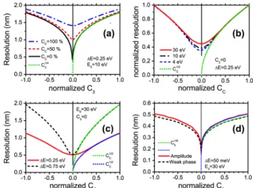
objects [18] as commonly encountered in LEEM and extract the resolution. We use E0¼0:25 eV and the column energyE¼15 keV. Figure1(a)shows resolution versus C3 (normalized to the uncorrected value) withCc ranging from uncorrected (100%) to fully corrected (0%). As Cc decreases, a deep cusp develops nearC3¼0. The minimum does not reach zero, as higher order coefficients [17] (such as Ccc, andC5) are set at the nonzero values obtained from ray tracing. The minimum is shifted to a slightly negative value ofC3, offsetting the positive value ofC5. The dottedC1=43 line is in close agreement with the full calculations when Cc¼0. These results do not depend significantly onE0. The effects of nonzero defocus will be discussed in more detail below.

In Fig.1(b)C3 ¼0andCcis varied for different values ofE0. The dotted line shows/C1=2c . For all values ofE0, as Cc increases the simulations follow /C1=2c closely. Figure1(c)comparesE0 ¼0:25 eV(cold field emission [19]) with E0¼0:75 eV (typical LaB₆ gun [20]). The ordinate is not normalized, to highlight differences on an absolute scale. Dotted lines are individually scaled C1=2c lines. While near Cc ¼0 the two cases are al-most identical, for the uncorrected situation the difference is significant. As expected, the minimum is steeper and

FIG. 1 (color online). (a) Resolution of an amplitude object versus the normalized value of C3, for different settings of Cc

(uncorrected, 100%; fully corrected, 0%). Start energy E0¼ 10 eV, E0¼0:25 eV. Green dotted line: C13=4 prediction of

Eqs. (2b) and (4b). (b) Resolution (normalized to uncorrected values) versus normalized value ofCc, withC3¼0, forE0¼4,

10, and 30 eV. (c) Resolution versus normalized value of Cc,

with C3¼0, for E0¼0:25 and 0.75 eV. Dotted lines in (b)

and (c): C1c=2 prediction of Eqs. (2a) and (6b). (d) Resolution

versusC5forCc=C3corrected LEEM withE0¼50 meV. The

narrower as E0 increases and chromatic aberration is more significant. Very similar results were obtained for weak-phase objects [18] or by plotting point resolution [Eq. (4)] versusC3 for amplitude and weak-phase objects. Finally, in Fig. 1(d) we consider a ‘‘supercorrected’’ LEEM in whichCc¼C3¼0. The remaining chromatic aberrations are minimized by an energy-filtered gun with

E0¼50 meV. The cusp aroundC5 ¼0shows the pre-dictedC1=6₅ dependence. This microscope promises atomic resolution (0.17 nm) with 30 eV electrons, limited by the higher order chromatic terms. It is conceivable that such an instrument can be designed and built, using an electron mirror with at least four electrostatic elements to control C1, C3,C5, and Cc.C5 must be reduced from 14.5 m to <0:5 mm[17],C3from300 mmto 10m, with a stability of0:5m, andC1 must be controlled to better than 2 nm. However, the corrected state would be ex-tremely fragile due to the very steep and narrow cusp in Fig.1(d).

Turning to transmission microscopes, the C3-limited TEM resolution at Scherzer defocus is given [15] by¼

0:66C1=4₃ 3=4, the sameC1=4₃ dependence as seen before. In the following we focus on the region of slightly negative C3 and slightly positiveC1, which previous studies have shown to give the highest resolution imaging results. Figure2(a)shows the point resolution [the qvalue at the first zero crossing of sinð2Þ, in nm1] versus C3 for a weak-phase object in a microscope similar to the so-called TEAM instrument [2] (C5 ¼5 mm, 300 keV). We note the presence of a narrow, ridge-shaped optimum-resolution band diagonally across the figure, with optimum performance along the solid yellow line near the center. The CTF along this line is optimally balanced over all spatial frequencies below the point resolution and is char-acterized by a single parameter, 0< < =2 (see the Supplemental Material [21]). At¼=2, Fig.2(a)shows a singularity where two line-shaped singularities intersect. To the right of this point the resolution is always inferior. Along the white dashed line the CTF becomes unstable and the resolution drops abruptly. The distance between the yellow line and the white line is the largest deviation that can be tolerated without a significant loss of resolution, defining an ‘‘instability budget’’ for C1 and C3 (see the Supplemental Material [21]). Figure 2(b) plots the insta-bility budgets as a function of . The budget for C1 decreases from 0:7 nm at ¼=32 to 0 nm at ¼ =2, while forC3it changes from1mto0 m. At the same time,changes from 46 pm at¼=32to 38 pm at ¼=2. Note that these instability budgets are not fixed: they depend on the value of selected by the operator. Figure2(c)shows the CTF for¼=32,=4, and=2. For¼=4(Scherzer defocus) the instability budgets for C1andC3are0:28 nmand0:32m, respectively. For ¼=32, the resolution is somewhat worse, but stability has improved. In Figs.2(d) and 2(e) we plot the CTF at

¼=4[Fig.2(d)] and¼=32[Fig.2(e)], with addi-tional offsets inC1 of0:5 nm, exceeding the instability budget for¼=4, but well below it for¼=32. In Fig. 2(d)the CTF is strongly affected, with a deep mini-mum at q20 nm1 for 0:5 nm defocus. The CTF in Fig.2(e)is much less affected, with a point resolution well above 20 nm1 at 0:5 nm defocus, and 20 nm1 at

þ0:5 nm defocus. This may seem counterintuitive. To obtain 50 pm resolution, it would appear that the CTF at ¼=4 is better than at ¼=32, as it has a higher point resolution. However, it is also significantly less sta-ble. In practice, one may prefer the small loss in resolution at¼=32, as it provides a better instability budget. The map in Fig. 2(a) is not specific for a TEAM-like instru-ment. Every electron microscope whereC1andC3 can be adjusted for a given C5 behaves in the same manner. As shown in the Supplemental Material [21], the resolution scales withC1=6₅ , while the instability budgets forC1 and C3scale withC1=35 andC2=35 , respectively. The advent ofC3 correction led to an improvement in resolution by about a factor of 2. Could we gain another factor of 2 by reducing C5? The small inset labeled =2 in Fig. 2(a) shows the relative size of the resolution map resulting from a reduc-tion of C5 from 5 to 0.08 mm, required to improve the resolution by a factor of 2. Regardless of the fact that this would present huge, possibly insurmountable challenges in controlling numerous other aberrations, it is clear from the diminutive size of this map that the leading aberrations C1andC3could not be controlled with sufficient accuracy and stability to make such an improvement possible; the instability budgets have shrunken to near nothing.

When Cc is corrected the system is—to first order— insensitive to small fluctuations in the electron gun poten-tial. But when only C3 is corrected, a small shiftv in the electron gun potential V is equivalent to a focus shift

C1¼Ccv=V. To appreciate the difference between a high frequency ripple versus a static shift of the gun potential, we refer to Fig.2(f ). We useCc¼1:6 mm, an energy spreadE¼100 meV, and no high voltage (HV) ripple (solid black line). The slow dropoff forq >10 nm1 is due to the chromatic envelope function, Eq. (5). The dashed line results when—in addition to the energy spread of 100 meV—we introduce an additional high voltage ripple of 60 mV. The effect is minor: a slightly stronger dropoff at higher qvalues. In contrast, the gray line uses

E¼100 meV, no HV ripple, plus a static HV shift of

final beam energy. However, instabilities in the accelera-tion stage (i.e., drift in the high tension supply for the electron gun) remain unremedied. A similar effect is caused by instabilities in the objective lens current I: a small current shifticauses a defocus shiftC1 ¼2Cci=I.

Thus, the objective lens power supply must have a relative stability of 5108. Such extraordinary long-term drift stabilities are extremely difficult to realize experimentally. For a TEAM-like instrument, the gun high voltage can drift over 100 mV on a time scale from minutes to hours, FIG. 2 (color online). (a) Point resolution (innm1) versusC1andC3nearC3¼0. Solid yellow line: Optimized performance as a

function of, ranging from¼0to=2. White dashed line: Abrupt instability in the transfer function. The inset below the scale bar, labeled=2, shows the relative size of this map if resolution is improved by a factor of 2 by reduction ofC5. (b) Instability budgets

forC1andC3, defined by the distance between the yellow line and the white dashed line in (a), as a function of. (c) CTF for different

values of. (d) CTF at¼=4with negative (dashed gray) and positive (solid gray) 0.5 nm additional defocus. (e) As (d) for ¼=32. The sensitivity for a small defocus is greater in (d) than in (e), in agreement with (b). (f ) CTF at ¼=4 with

depending on the quality of the air conditioning in the room [23]. Of course, mechanical drift of the sample along the beam direction, as well as undulations in the thin sample foil, also give rise to defocus shifts.

These results are not limited to LEEM or TEM, but hold for any electron optical instrument. As more aberration coefficients are corrected, the widths of the cusps within which correction must be maintained become increasingly narrow. Our findings shed new light on the short-lived corrected state observed in state-of-the-art aberration-corrected TEM instruments [9–11]. With resolution exqui-sitely sensitive to the residual values of the aberration coefficients, even minute mechanical and electronic drifts are strongly amplified. Uncorrected chromatic aberrations can create a small ‘‘island of stability’’ around the cor-rected state. Figure1(a)shows that this island is reasonably broad whenCcis uncorrected. But whenCcis corrected it shrinks dramatically, leaving the improved corrected state much less protected. Additionally, as the quality of the corrected state is improved, it becomes increasingly diffi-cult to reliably put and keep the system into that state. To put the CTF at ¼=4 within 30% of the instability budget, we must measureC1 andC3 with sufficient accu-racy and know the value ofC5to better than 1.5%. When we reduceC5, increase in instability outstrips improvement in resolution, posing a fundamental limit on the resolution that is ultimately achievable.

While the intrinsic instability identified in this Letter presents a serious challenge, it may be possible to monitor the state of the microscope in real time and adjust the instrument settings ‘‘on the fly,’’ i.e., by dynamic feedback, to maintain the corrected condition, much like most air-craft flying today are inherently unstable without sophisti-cated electronic control systems. Identifying suitable measurable parameters to fully quantify the state of the microscope during routine sample observation is a task that presently remains unresolved.

The authors thank Phil Batson for useful discussions. We also thank the referees for their helpful comments. This research was funded in part by the Netherlands Organization for Scientific Research (NWO) via an NWO-Groot Grant (‘‘ESCHER’’).

[1] P. W. Hawkes, Biol. Cell 93, 432 (2001); Advances in Imaging and Electron Physics: Aberration-corrected Electron Microscopy, edited by P. W. Hawkes (Academic, Amsterdam, 2008), Vol. 153.

[2] C. Kisielowskiet al., Microsc. Microanal.14, 78 (2008); J. C. Meyer, C. Kisielowski, R. Erni, M. D. Rossell, M. F. Crommie, and A. Zettl,Nano Lett.8, 3582 (2008). [3] R. M. Tromp, J. B. Hannon, A. W. Ellis, W. Wan, A. Berghaus, and O. Schaff, Ultramicroscopy 110, 852 (2010); Th. Schmidt et al., Ultramicroscopy 110, 1358 (2010).

[4] R. Ko¨nenkamp, R. C. Word, G. F. Rempfer, T. Dixon, L. Almaraz, and T. Jones,Ultramicroscopy110, 899 (2010). [5] J. Zach and M. Haider,Nucl. Instrum. Methods Phys. Res.,

Sect. A363, 316 (1995).

[6] S. Itose, M. Matsuya, S. Uno, K. Yamashita, S. Ebata, M. Ishihara, K. Uchino, H. Yurimoto, K. Sakaguchi, and M. Kudo, Microsc. Microanal. Suppl. S2, 17, 654 (2011).

[7] E. Munro, J. Rouse, H. Liu, and L. Wang, J. Vac. Sci. Technol. B26, 2331 (2008).

[8] H. H. Rose,Phil. Trans. R. Soc. A₃₆₇, 3809 (2009). [9] J. Barthel and A. Thust,Ultramicroscopy111, 27 (2010). [10] J. Biskupek, P. Hartel, M. Haider, and U. Kaiser,

Ultramicroscopy116, 1 (2012).

[11] P. Ercius, M. Boese, Th. Duden, and U. Dahmen,Microsc. Microanal.18, 676 (2012).

[12] G. Rempfer,J. Appl. Phys.67, 6027 (1990); G. Rempfer and M. S. Mauck, Optik92, 3 (1992).

[13] M. Haider, S. Uhlemann, E. Schwan, H. Rose, B. Kabius, and K. Urban, Nature (London) 392, 768 (1998); O. L. Krivanek, N. Dellby, and A. R. Lupini, Ultramicroscopy

78, 1 (1999).

[14] M. Haider, H. Mu¨ller, S. Uhlemann, J. Zach, U. Loebau, and R. Hoeschen,Ultramicroscopy108, 167 (2008). [15] D. B. Williams and C. B. Carter, Transmission Electron

Microscopy: A Textbook for Materials Science(Springer, New York, 2009), 2nd ed.

[16] S. M. Schramm, A. B. Pang, M. S. Altman, and R. M. Tromp,Ultramicroscopy115, 88 (2012).

[17] R. M. Tromp, W. Wan, and S. M. Schramm, Ultramicroscopy119, 33 (2012).

[18] A. B. Pang, Th. Mu¨ller, M. S. Altman, and E. Bauer, J. Phys. Condens. Matter21, 314006 (2009).

[19] R. M. Tromp, M. Mankos, M. C. Reuter, A. W. Ellis, and M. W. Copel,Surf. Rev. Lett.5, 1189 (1998).

[20] L. H. Veneklasen,Ultramicroscopy36, 76 (1991). [21] See the Supplemental Material at http://link.aps.org/

supplemental/10.1103/PhysRevLett.109.163901 for a more detailed description of the behavior of the CTF in the vicinity of the yellow line in Fig. 2(a) and for a derivation of the instability budgets.