5919.pdf

GRANGER CAUSALITY IN MIXED FREQUENCY TIME SERIES

Kaiji Motegi

A dissertation submitted to the faculty of the University of North Carolina at Chapel

Hill in partial fulfillment of the requirements for the degree of Doctor of Philosophy in

the Department of Economics.

Chapel Hill

2014

Approved by:

Eric Ghysels

Michael Aguilar

Saraswata Chaudhuri

Neville Francis

c

°

2014

Kaiji Motegi

ABSTRACT

Kaiji Motegi: Granger Causality in Mixed Frequency Time Series

(Under the direction of Eric Ghysels)

It is a classic topic in time series econometrics to test Granger causality among multiple

variables. While many Granger causality tests have been invented in the literature, they are

often vulnerable to temporal aggregation which potentially generates or hides causality. Based

on the growing literature of Mixed Data Sampling (MIDAS) analysis, this dissertation proposes

a set of mixed frequency Granger causality tests which are robust against temporal aggregation.

The mixed frequency causality tests take an explicit treatment of data sampled at different

frequencies, and hence enable more accurate statistical inference than the conventional approach

that aggregates all time series into the common lowest frequency.

Depending on the magnitude of the ratio of sampling frequencies, this dissertation proposes

two types of mixed frequency causality tests. The first one handles a small ratio of sampling

frequencies like month vs. quarter. Exploiting Ghysels’ mixed frequency vector autoregressive

(MF-VAR) models, we extend Dufour, Pelletier, and Renault’s VAR-based causality test to

the mixed frequency context. We prove that the mixed frequency approach better recovers the

underlying causal patterns than the existing low frequency approach. Moreover, we demonstrate

via local asymptotic power analysis and simulations that the mixed frequency test has higher

power than the low frequency test in both large sample and small sample. In an empirical

application on U.S. macroeconomy, we show that the mixed frequency approach and the low

frequency approach produce very different causal implications, with the former yielding more

intuitive results.

ACKNOWLEDGEMENTS

TABLE OF CONTENTS

LIST OF TABLES . . . .

ix

LIST OF FIGURES . . . .

x

1

INTRODUCTION . . . .

1

2

VAR-BASED TEST . . . .

3

2.1

Introduction

. . . .

3

2.2

Mixed Frequency Data Model Specifications

. . . .

4

2.2.1

Brief Literature Review . . . .

5

2.2.2

Mixed Frequency VAR Models . . . .

6

2.2.3

Estimators and Their Large Sample Properties . . . 10

2.3

Testing Causality with Mixed Frequency Data

. . . 13

2.3.1

Preliminaries . . . 13

2.3.2

Causality Tests in Mixed Frequency VAR Models

. . . 16

2.4

Recovery of High Frequency Causality . . . 20

2.4.1

Temporal Aggregation of VAR Processes

. . . 20

2.4.2

Causality and Temporal Aggregation

. . . 24

2.5

Local Asymptotic Power Analysis

. . . 28

2.6

Power Improvements in Finite Samples . . . 33

2.6.1

Bivariate Case

. . . 34

2.6.2

Trivariate Case

. . . 38

2.8

Concluding Remarks . . . 44

3

REGRESSION-BASED TEST . . . .

56

3.1

Introduction

. . . 56

3.2

Methodology . . . 58

3.2.1

High-to-Low Granger Causality

. . . 59

3.2.2

Low-to-High Granger Causality

. . . 66

3.3

Local Asymptotic Power Analysis

. . . 68

3.4

Monte Carlo Simulations

. . . 76

3.4.1

High-to-Low Causality

. . . 76

3.4.2

Low-to-High Causality

. . . 79

3.5

Empirical Application . . . 82

3.6

Conclusions . . . 86

A TECHNICAL APPENDICES FOR CHAPTER 2 . . . .

95

A.1 Asymptotic Properties of MF-VAR Parameter Estimators . . . 95

A.1.1

Least Squares Estimator and Asymptotic Variance . . . 95

A.1.2

Proof of Theorems 2.2.1 and 2.2.2

. . . 101

A.2 Proof of Theorem 2.4.1

. . . 103

A.3 Proof of Theorem 2.4.2

. . . 104

A.4 Proof of Theorem 2.4.3

. . . 105

B TECHNICAL APPENDICES FOR CHAPTER 3 . . . 106

B.1 Double Time Indices . . . 106

B.2 Autocovariance Structures of

x

and

x

. . . 107

B.2.1

Preliminaries . . . 107

B.2.2

Mixed Frequency Models

. . . 108

B.3 Proof of Theorem 3.2.1

. . . 112

B.4 Proof of Theorem 3.2.2

. . . 114

B.5 Proof of Theorem 3.2.3

. . . 115

B.6 Proof of Theorem 3.2.4

. . . 118

B.7 Proof of Theorem 3.3.1

. . . 121

B.8 Proof of Theorem 3.3.3

. . . 123

LIST OF TABLES

2.1

Linear Parametric Restrictions of Non-causality . . . 46

2.2

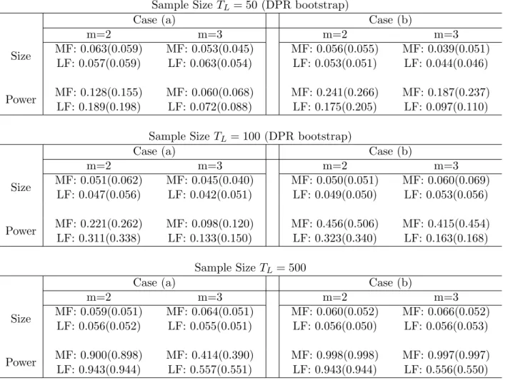
Rejection Frequencies (Bivariate VAR with i.i.d. Error and DPR Bootstrap) . . . 47

2.3

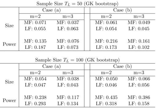
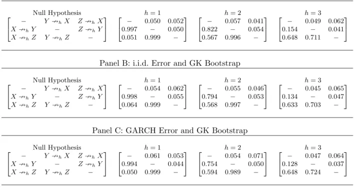
Rejection Frequencies (Bivariate VAR with i.i.d. Error and GK Bootstrap)

. . . 48

2.4

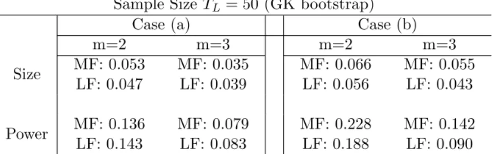
Rejection Frequencies (Bivariate VAR with GARCH Error and GK Bootstrap) . 49

2.5

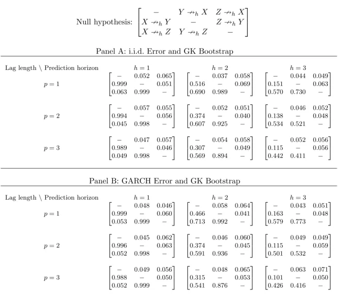
Rejection Frequencies for Trivariate MF-VAR . . . 50

2.6

Rejection Frequencies for Trivariate LF-VAR (Flow Sampling)

. . . 51

2.7

Rejection Frequencies for Trivariate LF-VAR (Stock Sampling) . . . 52

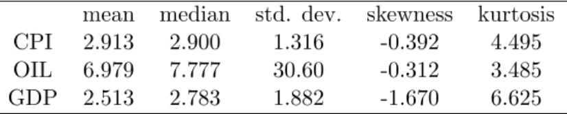
2.8

Sample Statistics . . . 52

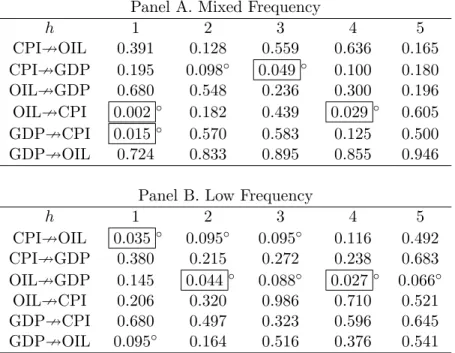
2.9

Granger Causality Tests for CPI, OIL, and GDP . . . 53

3.1

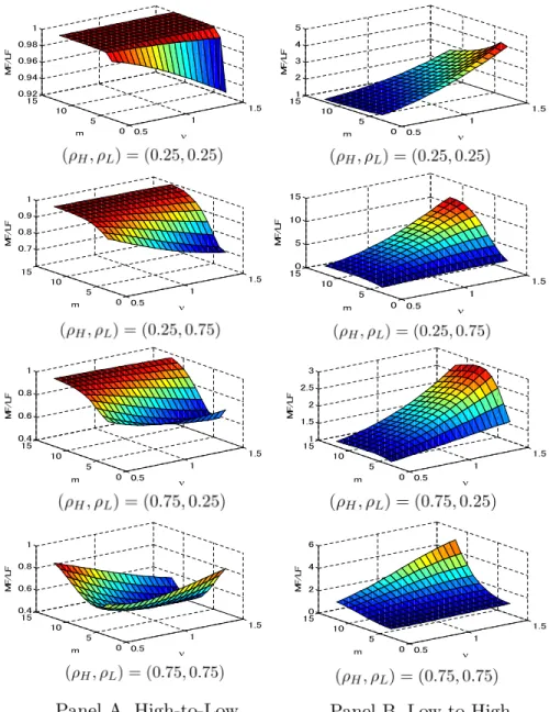
Local Asymptotic Power of Max Test and Wald Test (High-to-Low Causality) . . 87

3.2

Local Asymptotic Power of Max Tests (High-to-Low Causality) . . . 88

3.3

Rejection Frequencies of Max Test and Wald Test (High-to-Low Causality)

. . . 89

3.4

Rejection Frequencies of Max Test for Low-to-High Causality . . . 90

LIST OF FIGURES

2.1

Local Asymptotic Power of Mixed and Low Frequency Causality Tests . . . 54

2.2

Plot of the Function

mρ

- Driver of Local Asymptotic Power Ratios . . . 55

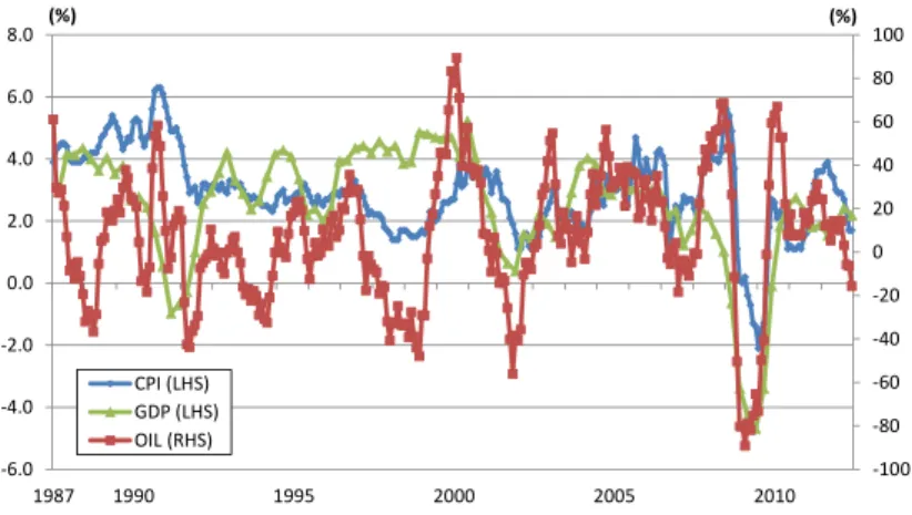
2.3

Time Series Plot of CPI, OIL, and GDP . . . 55

3.1

Time Series Plot of U.S. Interest Rates and Real GDP Growth . . . 93

CHAPTER 1

INTRODUCTION

It is a classic topic in time series econometrics to test Granger’s (1969) causality among multiple

variables. Many kinds of Granger causality tests have been invented in the past fifty years, and

the most prominent ones include Dufour, Pelletier, and Renault’s (2006) test based on vector

autoregression (VAR) models and Sims’ (1972) regression-based test. A well-known problem of

these existing tests is that they are often vulnerable to temporal aggregation which potentially

generates or hides causality, as noted in Granger (1980) and Granger (1988) among many others.

Such a misleading causality is called

spurious causality

(cfr. Dufour and Renault (1998)). Since

economic time series are often sampled at different frequencies (e.g. daily financial variables,

monthly business-cycle indicators, quarterly gross domestic product), we need new causality

tests that can control spurious causality.

To this end, we propose mixed frequency causality tests based on the growing literature of

Mixed Data Sampling (MIDAS) analysis. Originated with Ghysels, Santa-Clara, and Valkanov

(2004), Ghysels, Santa-Clara, and Valkanov (2006), etc., the MIDAS approach works on data

sampled at different frequencies instead of working on data aggregated to the common lowest

frequency. By expanding the notion of Granger causality into the MIDAS framework, this

dis-sertation establishes mixed frequency Granger causality tests which give us improved statistical

accuracy, namely higher power, than the conventional low frequency approach does.

the mixed frequency framework. We prove that the mixed frequency approach better

recov-ers the underlying causal patterns than the existing low frequency approach. Moreover, we

demonstrate via local asymptotic power analysis and Monte Carlo simulations that the mixed

frequency test has higher power than the low frequency test in both large sample and small

sample. In an empirical application involving U.S. macroeconomic indicators, we show that

the mixed frequency approach and the low frequency approach produce very different causal

implications, with the former yielding more intuitive results.

The second part of this dissertation deals with a relatively large ratio of sampling frequencies

like month vs. year (

m

= 12). Inspired by Sims’ (1972) regression-based causality tests and

Andrews and Ploberger’s (1994) optimal tests involving a nuisance parameter, we develop a

new test that achieves higher power than the conventional test in both large sample and small

sample. We combine multiple parsimonious regression models where the

i

-th model regresses a

low frequency variable

xL

onto the

i

-th high frequency lag or lead of a high frequency variable

xH

for

i

∈ {

1

, . . . , h

}

.

Let ˆ

βi

be an estimator for the loading of the

i

-th high frequency

lag or lead, then our test statistic basically takes the maximum among

{

β

ˆ

1

, . . . ,

β

ˆ

}

. In this

CHAPTER 2

VAR-BASED TEST

2.1

Introduction

It is well known that temporal aggregation may have spurious effects on testing for Granger

causality, as noted by Clive Granger himself in a number of papers, see e.g. Granger (1980),

Granger (1988), Granger (1995). In this paper we deal with what might be an obvious, yet

largely overlooked remedy. Time series processes are often sampled at different frequencies and

then typically aggregated to the common lowest frequency to test for Granger causality. The

analysis of the present paper pertains to comparing testing for Granger causality with all series

aggregated to the common lowest frequency, and testing for Granger causality taking advantage

of all the series sampled at whatever frequency they are available. We rely on mixed frequency

vector autoregressive models to implement a new class of Granger causality tests.

We show that mixed frequency Granger causality tests better recover causality patterns in

an underlying high frequency process compared to the traditional low frequency approach. We

also formally prove that mixed frequency causality tests have higher asymptotic power against

local alternatives and show via simulation that this also holds in finite samples involving realistic

data generating processes. The simulations indicate that the mixed frequency VAR approach

works well for small differences in sampling frequencies - like quarterly/monthly mixtures.

We apply the mixed frequency causality test to monthly inflation, monthly crude oil price

1

fluctuations, the real GDP growth in the U.S. We also apply the conventional low frequency

causality test to the aggregated quarterly price series and real GDP for comparison. These

two approaches yield very different causal implications.

In particular, significant causality

from oil prices to inflation is detected by the mixed frequency approach but not by the low

frequency approach. The result suggests that the quarterly frequency is too coarse to capture

such causality.

The paper is organized as follows. In Section 2.2 we first briefly review the Granger causality

and MIDAS literatures and then frame mixed frequency VAR models. In Section 2.3 we

de-velop the mixed frequency causality tests. Section 2.4 discusses how we can recover underlying

causality using a mixed frequency approach compared to a traditional low frequency approach.

Section 2.5 shows that the mixed frequency causality tests have higher local asymptotic power

than the low frequency ones do. Section 2.6 reports Monte Carlo simulation results and

doc-uments the finite sample power improvements achieved by the mixed frequency causality test.

In Section 2.7 we apply the mixed frequency and low frequency causality tests to U.S.

macroe-conomic data. Finally, Section 2.8 provides some concluding remarks. All tables and Figures

are provided after Section 2.8. Proofs for all theorems as well as some theoretical details are

provided in Technical Appendices A.

2.2

Mixed Frequency Data Model Specifications

In this section we frame a mixed frequency vector autoregressive (henceforth MF-VAR) model

and derive some asymptotic properties. We first provide a short review of the related literature.

We then formally present the MF-VAR model. Finally, we establish large sample results for

parameter estimators and corresponding Wald statistics.

We will use the following notational conventions throughout. Let

A

∈ R

. The

l

-norm

is

|

A

|

:= (

P

P

a

)

= (tr[A

A])

; the

L

-norm is

k

A

k

:= (

P

P

j=1

E

|

a

|

)

;

2.2.1

Brief Literature Review

The notion of causality introduced by Granger (1969) is defined in terms of incremental

pre-dictive ability, beyond the past observations of a time series process

X,

by past observations of

another time series process

Y.

Although so-called

Granger causality

has been extended to fairly

general settings including nonlinear and random volatility models, it is typically discussed in a

linear regression framework, in particular since Sims (1972).

Early contributions by Zellner and Montmarquette (1971) and Amemiya and Wu (1972)

pointed out the potentially adverse effects of temporal aggregation on testing for Granger

causality. The subject has been extensively researched ever since, e.g. Granger (1980), Granger

(1988), L¨

utkepohl (1993), Granger (1995), Renault, Sekkat, and Szafarz (1998), Marcellino

(1999), Breitung and Swanson (2002), McCrorie and Chambers (2006), Silvestrini and Veredas

(2008), among others. It is worth noting that whenever Granger causality and temporal

aggre-gation are discussed, it is typically done in a setting where

all

series are subject to temporal

aggregation. In such a setting it is well-known that even the simplest models, like a

bivari-ate VAR(1) with stock (or skipped) sampling, may suffer from spuriously hidden or generbivari-ated

causality, and recovering the original causal pattern is very hard or even impossible in general.

As in the single frequency VAR literature, exploring mixed frequency Granger causality

among more than two variables invariably relates to the notion of multi-horizon causality studied

by L¨

utkepohl (1993), Dufour and Renault (1998) and Hill (2007). Of direct interest to us is

Dufour and Renault (1998) who generalized the original definition of single-horizon or short run

causality to multiple-horizon or long run causality to handle causality chains: in the presence of

an auxiliary variable

Z

,

Y

may be useful for a multiple-step ahead prediction of

X

even if it is

useless for the one-step ahead prediction. Dufour and Renault (1998) formalize the relationship

between VAR coefficients and multiple-horizon causality and Dufour, Pelletier, and Renault

(2006) formulate accordingly single step Wald tests of multiple-horizon non-causality. Their

framework will be used extensively in our analysis. See Hill (2007) for a sequential method of

testing for multiple-horizon non-causality.

Santa-Clara, and Valkanov (2005). A number of papers have linked MIDAS regressions to

(latent) high frequency VAR models, such as Foroni, Marcellino, and Schumacher (2013) and

Kuzin, Marcellino, and Schumacher (2011), whereas Ghysels (2012) discusses the link between

mixed frequency VAR models and MIDAS regressions. None of these papers study in any detail

the issue of Granger causality.

2.2.2

Mixed Frequency VAR Models

We want to characterize three settings which we will refer to as HF, MF and LF - respectively

high, mixed and low frequency. We begin by considering a partially latent underlying HF

process. Using the notation of Ghysels (2012), the HF process contains

{{

x

(

τL, k

)

}

}

and

{{

x

(

τ

, k

)

}

}

, where

τ

∈ {

0

, . . . , T

}

is the LF time index (e.g. quarter),

k

∈ {

1

,

. . . , m

}

denotes the HF (e.g. month), and

m

is the number of HF time periods between LF

time indices. In the month versus quarter case, for example,

m

equals three since one quarter

has three months. Observations

x

(

τ

, k

)

∈ R

,

K

≥

1, are called HF variables, whereas

x

(

τ

, k

)

∈ R

,

K

≥

1, are latent LF variables because they are not observed at high

frequencies - as only some temporal aggregates are available.

Note that two simplifying assumptions have implicitly been made. First, there are assumed

to be only two sampling frequencies. Second, it is assumed that

m

is fixed and does not depend

on

τL.

Both assumptions can be relaxed at the cost of much more complex notation and algebra

which we avoid for expositional purpose - again see Ghysels (2012).

In reality the analyst’s choice is limited to MF and LF cases. Only low frequency variables

have been aggregated from a latent HF process in a MF setting, whereas both low

and

high

frequency variables are aggregated from the latent HF process to form a LF process. Following

L¨

utkepohl (1987) we consider only linear aggregation schemes involving weights

w

= [

w1, . . . ,

wm

]

such that:

x

(

τ

) =

X

k=1

w

x

(

τ

, k

) and

x

(

τ

) =

X

k=1

w

x

(

τ

, k

).

(2.2.1)

w

=

I

(

k

=

m

); and (2)

flow

sampling, where

w

= 1 for

k

= 1

, . . . , m

.

In summary, we

observe:

•

all high and low frequency variables

{{

x

(

τL, j

)

}

}

and

{{

x

(

τL, j

)

}

j=1

}

in a HF

process;

•

all high frequency variables

{{

x

(

τ

, j

)

}

}

but only aggregated low frequency

vari-ables

{

x

(

τL

)

}

in a MF process;

•

only aggregated high and low frequency variables

{

x

(

τ

)

}

and

{

x

(

τ

)

}

in a LF

process.

A key idea of MF-VAR models is to stack everything observable given a MF process

ac-cording to their order over time. This results in the following

K

=

KL

+

mKH

dimensional

vector:

X

(

τL

) = [x

(

τL,

1)

, . . . ,

x

(

τL, m

)

,

x

(

τL

)

]

.

(2.2.2)

Note that

x

(

τ

) is the last block in the stacked vector - a conventional assumption implying

that it is observed after

x

(

τ

, m

)

.

Any other order is conceptually the same, except that it

implies a different timing of information about the respective processes. We will work with the

specification appearing in (2.2.2) as it is most convenient.

Example 1

:

Quarterly Real GDP

: A leading example of how a mixed frequency model is

useful in macroeconomics concerns quarterly real GDP growth

xL

(

τL

), where existing studies of

causal patterns use monthly unemployment, oil prices, inflation, interest rates, etc. aggregated

into quarters (see Hill (2007) for references). Consider the monthly oil price changes and CPI

inflation [x

(

τ

,

1)

,

. . .

,

x

(

τ

,

3)

]

, which will be actually analyzed in Section 2.7. Note that

τ

represents a quarter and

x

is a 2

×

1 vector. According to the Bureau of Economic Analysis,

GDP is announced in advance roughly one month after the quarter, with subsequent updates

over the following two months (e.g. the 2014 first quarter advanced estimate is due April 30,

2014). By comparison, oil prices are available on a daily basis and hence their monthly data

2_{One can equivalently let w}

k = 1/m for k = 1, . . . , m in flow sampling if the average is preferred to a

can be calculated immediately after the month. Also, the monthly CPI is announced roughly

three weeks after the month. Since the two monthly series are announced before the GDP, the

ordering is exactly as shown in (2.2.2).

In order to proceed, we will make a number of standard regulatory assumptions. Let

F

≡

σ

(X

(

t

) :

t

≤

τ

). In particular we assume

E

[X

(

τ

)

|F

] has a version that is

almost surely

linear in

{

X

(

τ

−

1)

, ...,

X

(

τ

−

p

)

}

for some finite

p

≥

1.

Assumption 2.2.1.

The process

X

(

τ

) is governed by a VAR(

p

) for some

p

≥

1:

X

(

τ

) =

X

k=1

A

X

(

τ

−

k

) +

²(

τ

)

.

(2.2.3)

The coefficients

A

are

K

×

K

matrices for

k

= 1

, . . . , p

. The

K

×

1 error vector

²(

τ

) =

[

²1

(

τ

),

. . .

,

²

(

τ

)]

is a strictly stationary martingale difference with respect to increasing

F

⊂ F

, where

Ω

≡

E

[²(

τL

)²(

τL

)

] is positive definite.

Remark 1.

Martingale difference errors

E

[²(

τ

)

|F

] =

0

allow for conditional

heteroskedas-ticity of unknown form. Nevertheless, in order to test for non-causality using (2.2.3) we estimate

a parameter subset from a (

p, h

)-autoregression defined in (2.2.5), below. Asymptotics for

M-estimators of the resulting parameter involve finite sums of martingale differences which are not

in general martingale differences, and anyway the martingale difference property alone does not

suffice for Gaussian asymptotics of M-estimators (cf. McLeish (1974), Hall and Heyde (1980)).

We therefore impose a mixing condition in Assumption 2.2.3 below.

Remark 2.

Unless

{

²(

τ

)

}

is an i.i.d. process, the VAR coefficients

A

do not necessarily carry

all the usual information about higher order causation, including volatility spillover (cfr. King,

Sentana, and Wadhwani (1994), Caporale, Pittis, and Spagnolo (2006)). This is irrelevant for

our purposes, however, because in the tradition of Dufour and Renault (1998) our analysis is

primarily about deducing nonlinear restrictions on

{

A

, ...,

A

}

that relate information about

Remark 3.

We assume the lag order

p

is either known, or the true order resulting in a

martingale difference error

²(

τ

) is at least as large as

p

. In practice standard methods for

selecting the lag apply in a mixed frequency environment, including tests of white noise. Indeed,

in general regression model specification tests easily extend to mixed frequency data. A large lag

order and/or a large number of variables, moreover, may lead to empirical size distortions in our

asymptotic chi-squared test statistic. This is particularly relevant in a mixed frequency VAR

since

m

and therefore

K

may be large. This topic is well known with bootstrap-based solutions

(e.g. Dufour, Pelletier, and Renault (2006) when regression errors are i.i.d, and Gon¸

calves

and Killian (2004) when errors may be heteroskedastic of unknown form). See Section 2.6,

below where simulation evidence clearly shows a bootstrap approach for approximating our

test statistic’s critical values work well.

In addition, the following standard assumptions ensure stationarity and

α

-mixing of the

observed time series and the MF-VAR errors.

Define

G

≡

σ

(

{

X

(

i

)

,

²(

i

)

}

:

s

≤

i

≤

t

) and

mixing coefficients

α

≡

sup

−∞,B⊂G∞t+h

|

P

(

A ∩ B

)

−

P

(

A

)

P

(

B

)

|

(cfr. Rosenblatt (1956) and

Ibragimov (1975)).

Assumption 2.2.2.

All roots of the polynomial det(I

−

P

A

z

k

_{) = 0 lie outside the unit}

circle.

Assumption 2.2.3.

X

(

τ

) and

²(

τ

) are

α

-mixing:

P

h=0

α

<

∞

.

Remark 4.

Recall that

α

-mixing implies mixing in the ergodic sense, and therefore ergodicity

(see Petersen (1983)). Hence by Assumptions 2.2.1-2.2.3

{

X

(

τL

)

,

²(

τL

)

}

are stationary and

ergodic.

Remark 5.

Asymptotics for our estimator only requires

P

α

<

∞

because under

Assump-tions 2.2.1 and 2.2.2

X

(

τL

) has a positive bounded spectral density (cfr. Ibragimov (1975)).

This allows for geometric memory decay

αh

=

O

(

ρ

) for some

ρ

∈

(0

,

1), as well as much

slower decay and therefore persistence since

αh

=

O

(

h

) for tiny

ι >

0 suffices for Gaussian

asymptotics (cfr. Ibragimov (1975)). Our Wald statistic requires a greater constraint on the

3_{Although a large body of literature exists on Granger causality in non-stationary or cointegrated systems}

mixing coefficients

α

due to a kernel variance estimator: see Theorem 2.2.2 and Appendix

A.1.1, below.

Remark 6.

A mixing property for the scalar components of the error

²(

τ

) covers a great

variety of conditional volatility processes including GARCH and many asymmetric GARCH

processes (e.g. Boussama (1998), Carrasco and Chen (2002), Meitz and Saikkonen (2008)).

Conditions for geometric ergodicity and therefore

α

-mixing for the BEKK class of multivariate

strong GARCH(

p, q

) processes are known and carry over to a latent HF multivariate GARCH(

p,

q

) process (see Boussama, Fuchs, and Stelzer (2011)). Any finite lag measurable transform of

α

-mixing

²(

τL

) is

α

-mixing, hence the mixing property for the HF process carries over to the MF

process. If

²(

τL

) is i.i.d. and has a continuous bounded joint distribution then from stationarity

Assumption 2.2.2 it follows

X

(

τL

) is geometrically

α

-mixing (see

§

2.3.1 in Doukhan (1994)).

Otherwise in general an

α

-mixing property for

²(

τ

) implies

X(

τ

) is also

α

-mixing when the

joint distribution of

²(

τ

) conditional on its history is absolutely continuous and bounded

almost

surely

(see

§

2.3.2 in Doukhan (1994)).

Note also that we do not include a constant term in (2.2.3) solely to reduce notation, thus

X

(

τL

) should be thought of as a de-meaned process. Finally, it is straightforward to allow an

infinite order VAR structure, and estimate a truncated finite order VAR model as in Lewis and

Reinsel (1985), L¨

utkepohl and Poskitt (1996), and Saikkonen and L¨

utkepohl (1996).

2.2.3

Estimators and Their Large Sample Properties

If the VAR(

p

) model appearing in (2.2.3) were standard, then the off-diagonal elements of

any matrix

A

would tell us something about causal relationships for some specific horizon.

The fact that MF-VAR models involve stacked replicas of high frequency data sampled across

different (high frequency) periods implies that potentially multi-horizon causal patterns reside

inside any of the matrices

A

.

It is therefore natural to start with a multi-horizon setting. We

do so, at first, focusing on multiple low frequency prediction horizons which we will denote by

h

∈ N

.

4

Another reason for studying multiple horizons is the potential of causality chains whenKH >1 orKL>1.

It is convenient to iterate (2.2.3) over the desired test horizon in order to deduce simple

testable parameter restrictions for non-causality. Recall that under Assumption 2.2.2 a unique

stationary and ergodic solution to (2.2.3) exists:

X

(

τ

) =

X

k=0

Ψ

²(

τ

−

k

)

,

(2.2.4)

where

Ψ

satisfies

Ψ

=

I

,

Ψ

=

P

s=1

A

Ψ

for

k

≥

1 and

Ψ

=

0

for

k <

0, and

|

Ψ

|

=

O

(

ρ

) for some

ρ

∈

(0

,

1). We then have what Dufour, Pelletier, and Renault (2006)

labeled as a (

p, h

)-autoregression:

X(

τL

+

h

) =

p

X

k=1

A

X

(

τL

+ 1

−

k

) +

h−1

X

k=0

Ψk

²(

τL

+

h

−

k

)

,

(2.2.5)

where

A

=

A

and

A

=

A

+

X

l=1

A

A

for

i

≥

2

.

By convention

A

=

0K

whenever

k > p.

The MF-VAR causality test exploits Wald statistics

based on the OLS estimator of the (

p, h

)-autoregression parameter set

B(

h

) =

h

A

, . . . ,

A

i

∈ R

_.

_(2.2.6)

If all variables were aggregated into a common low frequency and expanded into a (

p, h

)-autoregression, then

h

-step ahead non-causality has a simple parametric expression in terms

of

B(

h

); cfr. Dufour, Pelletier, and Renault (2006). Recall, however, that the MF-VAR has

a special structure because of the stacked HF vector. This implies that the Wald-type test

for non-causality that we derive is slightly more complicated than those considered by Dufour,

Pelletier, and Renault (2006) since in MF-VAR models the restrictions will often deal with

linear parametric restrictions across multiple equations. Nevertheless, in a generic sense we

show in Section 2.3 that non-causality between any set of variables in a MF-VAR model can be

expressed as linear constraints with respect to

B(

h

)

.

Hence, the null hypothesis of interest is a

linear restriction:

where

R

is a

q

×

pK

selection matrix of full row rank

q

, and

r

∈ R

.

We leave complete details

of the construction of

R

for Section 2.3.

The OLS estimator

B(

ˆ

h

) of

B(

h

) is

ˆ

B(

h

)

≡

arg min

B(h)

©

vec [U

(

h

)]

vec [U

(

h

)]

ª

=

£

W

(

h

)

W

(

h

)

¤

W

(

h

)

W

(

h

)

,

where

U

(

h

) is a matrix of stacked sums of

{

Ψ

}

and

{

²(

τ

)

}

while

W

(

h

) and

W

(

h

) are

matrices of stacked

{

X

(

τ

)

}

. See Appendix A.1.1 for derivation of

{

U

(

h

)

,

W

(

h

)

,

W

(

h

)

}

.

Assumptions 2.2.1-2.2.3 suffice for

B(

ˆ

h

) to be consistent for

B(

h

) and asymptotically

nor-mal. Limits are with respect to

T

→ ∞

hence

T

→ ∞

, where

T

=

T

−

h

+ 1 is the effective

sample size for the (

p, h

)-autoregression.

Theorem 2.2.1.

Under Assumptions 2.2.1-2.2.3

B(

ˆ

h

)

→

B(

h

) and

p

T

vec

h

ˆ

B(

h

)

−

B(

h

)

i

→

N

¡

0

,

Σp

(

h

)

¢

,

(2.2.8)

where

Σ

(

h

) is positive definite.

Remark 7.

See Appendix A.1.2 for a proof, and see Appendices A.1.1-A.1.2 for a complete

characterization of the asymptotic covariance matrix

Σ

(

h

).

If we have a consistent estimator

Σ

ˆ

(

h

) for

Σ

(

h

) which is

almost surely

positive

semi-definite for

T

≥

1, we can define the Wald statistic

W

[

H0

(

h

)]

≡

T

³

Rvec

h

ˆ

B(

h

)

i

−

r

´

×

³

R

Σp

ˆ

(

h

)R

´

×

³

Rvec

h

ˆ

B(

h

)

i

−

r

´

.

(2.2.9)

Implicitly, of course,

R

Σ

ˆ

(

h

)R

must be non-singular for any

R

∈ R

with full row rank.

In view of positive definiteness of

Σp

(

h

) by Theorem 2.2.1, and the supposition

Σp

ˆ

(

h

) =

Σp

(

h

)

+

op

(1), it follows (R

Σp

ˆ

(

h

)R

)

is well defined asymptotically with probability approaching

one.

We therefore obtain the following result, which we prove in Appendix A.1.2.

Remark 8.

A consistent,

almost surely

positive semi-definite estimator

Σ

ˆ

(

h

) is easily

con-structed by using Newey and West’s (1987) HAC estimator, given the stronger moment and

mixing conditions

||

²(

τL

)

||

<

∞

and

α

=

O

(

h

) for some

δ >

0. See Appendix A.1.1

for complete details.

In the remainder of the paper we will provide various tests for Granger causality which are

special cases of the generic framework derived so far.

2.3

Testing Causality with Mixed Frequency Data

In this section we define non-causality when data are sampled at mixed frequencies and describe

Wald-type tests associated with it. We first cover some preliminary notions of multiple-horizon

causality and extend it to the mixed sampling frequency case. We discuss in detail testing

non-causality from one variable to another, and whether they are high or low frequency variables.

We also cover non-causality from all high frequency variables to all low frequency variables and

vice versa, cases for which we give explicit formulae for the selection matrix

R

used in the null

hypothesis (2.2.7) and test statistic (2.2.9).

2.3.1

Preliminaries

We start with adopting the notion of non-causality to a mixed sampling frequency data filtration

setting. Using the notation of Dufour and Renault (1998) we define the relevant information

sets for the purpose of characterizing non-causality. In particular, let

L

be a Hilbert space

of covariance stationary real-valued random variables defined on a common probability space,

and the covariance as inner product. Moreover, let

I

(

τL

) be a closed increasing subspace of

L

such that

I

(

τ

)

⊂ I

(

τ

) whenever

τ

< τ

,

where

τ

, τ

∈ Z

.

Furthermore, define the indices

i

∈ {

1,

. . .

,

K

}

and

j

∈ {

1

, . . . , K

}

, and write ˜

x

(

τ

) =

[

x

(

τ

,

1)

, . . . , x

(

τ

, m

)]

. Note that ˜

x

(

τ

) is a vector

stacking

all

m

observations of the

i

-th high frequency variable available at period

τ

. We are putting a tilde in order to distinguish

it from the

aggregated

high frequency variable

x

(

τ

) =

P

k=1

w

x

(

τ

, k

) defined in (2.2.1).

Denote by

x(

−∞

, τ

] the Hilbert space spanned by

{

x(

τ

)

|

τ

≤

τ

}

.

The information set

I

is said to be

conformable

with

x

if

x(

−∞

, τ

]

⊂ I

(

τ

) for all

τ

.

We call the information

set derived from

I

(

τL

) =

X

(

−∞

, τL

], where

X(

τL

) is given in (2.2.2), as the

MF reference

information set in period

τL,

whereas

I

=

{I

(

τL

)

|

τL

∈ Z}

is the

MF reference information set

.

Therefore, the only information available up to period

τL

is the high frequency observations of

all high frequency variables and the low frequency observations of all low frequency variables.

In addition, let

I

denote the MF reference information set except for the

i

-th high frequency

variable

x

, and let

I

denote the information set except for

x

. Similarly,

I

is the

MF reference information set except for all high frequency variables

x

, . . . , x

.

I

is

the MF reference information set except for all low frequency variables

x

, . . . , x

. Note

that since the stacked high frequency observations ˜

x

(

τ

) and the low frequency observation

xL,j

(

τL

) belong to

X

(

τL

) for all

i

∈ {

1

, . . . , KH

}

and

j

∈ {

1

, . . . , KL

}

, it is clear that the MF

reference information set

I

=

{I

(

τL

)

|

τL

∈ Z}

is conformable with ˜

x

(

τL

) and

xL,j

(

τL

).

Finally, let

E

and

F

be two subspaces of

L

, and let

E

+

F

denote the Hilbert subspace

generated by the elements of

E

and

F.

Let

P

[x(

τ

+

h

)

| I

(

τ

)] be the best linear forecast of

x(

τ

+

h

) based on

I

(

τ

) in the sense of a covariance orthogonal projection.

For any generic information set and pair of processes (high or low frequency) the notion of

non-causality is defined as follows.

Definition 2.3.1.

(Non-causality at Different Horizons). Suppose that

I

is conformable with

x

.

(i)

y

does not cause

x

at horizon

h

given

I

(denoted by

y

9

x

| I

) if:

P

[x(

τL

+

h

)

|I

(

τL

)] =

P

[x(

τL

+

h

)

|I

(

τL

) +

y(

−∞

, τL

]]

∀

τL

∈ Z

.

Moreover, (ii)

y

does not cause

x

up to horizon

h

given

I

(denoted by

y

9

x

| I

) if

y

9

x

| I

for all

k

∈ {

1

, . . . , h

}

.

Definition 2.3.1 applies to a mixed sampling frequency setting when suitable information

set and processes are used.

Consider, for example, non-causality from the

j

-th low frequency

variable

x

to the

i

-th high frequency variable

x

. We say

x

does not cause

x

at horizon

5_{Definition 2.3.1 corresponds to Definition 2.2 in Dufour and Renault (1998) for covariance stationary}

h

given

I

(denoted by

x

9

x

| I

) if

P

[˜

x

(

τ

+

h

)

| I

(

τ

)] =

P

[˜

x

(

τ

+

h

)

| I

(

τ

) ] for

all

τ

∈ Z

. A key here is that we treat the

m

-dimensional stacked vector of

x

as one block.

This treatment allows us to apply Definition 2.3.1 to mixed frequency frameworks without any

theoretical complications.

When we consider non-causality between a pair of high frequency series, namely

xH,i1

9

x

| I

for

i

, i

∈ {

1

, . . . , K

}

, it should be noted that we focus exclusively on low frequency

horizons

h

, or equivalently horizons

h

×

m

. Any other horizon, not a multiple of

m

, is not

considered here. They can be handled with the existing same frequency setting of Dufour and

Renault (1998).

We often treat all

K

high frequency variables as a group and all

K

low frequency variables

as the other group, so provide the explicit definition of non-causality in such a case. We say all

low frequency variables do not cause all high frequency variables at horizon

h

given

I

(denoted

by

x

9

x

| I

) if

P

[˜

x

(

τL

+

h

)

| I

(

τL

)] =

P

[˜

x

(

τL

+

h

)

| I

(

τL

) ] for all

τL

∈ Z

, where

˜

x

(

τL

) = [˜

x

(

τL

)

,

. . .

, ˜

x

(

τL

)

]

.

In summary, there are six basic cases to consider in a mixed frequency setting.

Case 1 (low to low)

Non-causality from the

j1

-th

low

frequency variable,

xL,j1

, to the

j2

-th

low

frequency variable,

x

, at horizon

h

. The null hypothesis is written as

H

(

h

) :

x

9

x

| I

.

Case 2 (high to low)

H

0

(

h

) :

x

9

x

| I

.

Case 3 (low to high)

H

(

h

) :

xL,j1

9

xH,i1

| I

.

Case 4 (high to high)

H

(

h

) :

xH,i1

9

xH,i2

| I

.

Case I (all high to all low)

Non-causality from all high frequency variables

xH,1, . . . , xH,K

to all low frequency variables

xL,1, . . . , xL,K

at horizon

h

. The null hypothesis is written

as

H

(

h

) :

x

9

x

| I

.

Case II (all low to all high)

H

(

h

) :

x

9

x

| I

.

a bivariate system - causality chains can be excluded in both cases. In the bivariate system

non-causality at one horizon is synonymous to non-causality at all horizons (see Dufour and

Renault (1998: Proposition 2.3), cfr. Florens and Mouchart (1982: p. 590)). In order to avoid

tedious matrix notation, we do not treat in detail cases involving non-causation from a subset

of all variables to another subset. Our results straightforwardly apply, however, in such cases

as well.

2.3.2

Causality Tests in Mixed Frequency VAR Models

Our next task is to construct the selection matrices

R

for the various null hypotheses (2.2.7)

associated with the six generic cases. This requires deciphering parameter restrictions for

non-causation based on the (

p, h

)-autoregression appearing in equation (2.2.5).

Characterizing restrictions on

A

for each case above requires some additional matrix

notation. Let

N

∈ R

, and let

a, b, c, d, ι, ι

∈ {

1

, . . . , n

}

with

a

≤

b, c

≤

d,

and (

b

−

a

)

/ι

and (

d

−

c

)

/ι

being nonnegative integers.

Then we define

N(

a

:

ι

:

b, c

:

ι

:

d

) as the

(

+ 1)

×

(

+ 1) matrix which consists of the

a

-th, (

a

+

ι

)-th, (

a

+ 2

ι

)-th, . . . ,

b

-th rows and

c

-th, (

c

+

ι

)-th, (

c

+ 2

ι

)-th, . . . ,

d

-th columns of

N

.

Put differently,

a

signifies the first element

to pick,

b

is the last, and

ι

is the increment with respect to rows.

c

,

d

, and

ι

play analogous

roles with respect to columns. It is clear that:

N

(

a

:

ι

:

b, c

:

ι

:

d

)

=

N

(

c

:

ι

:

d, a

:

ι

:

b

)

.

(2.3.1)

A short-hand notation is used when

a

=

b

:

N(

a

:

ι

:

b, c

:

ι

:

d

) =

N(

a, c

:

ι

:

d

)

.

When

ι

= 1

,

we write:

N

(

a

:

ι

:

b, c

:

ι

:

d

) =

N

(

a

:

b, c

:

ι

:

d

)

.

Analogous notations are used when

c

=

d

or

ι

= 1, respectively.

By Theorem 3.1 in Dufour and Renault (1998) and from model (2.2.5), it follows that

H

(

h

)

are equivalent to:

A

(

a

:

ι

:

b, c

:

ι

:

d

) =

0

for each

k

∈ {

1

, . . . , p

}

,

(2.3.2)

II.

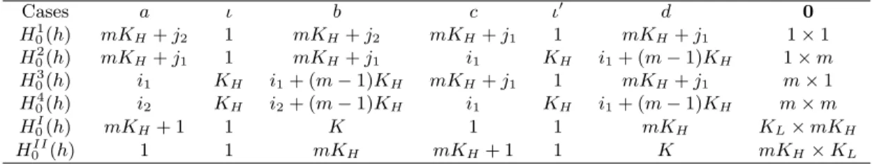
In Table 2.1 we detail the specifics for

a, ι, b, c, ι

, d

in these quantities for each of the six

cases.

Each case in Table 2.1 can be interpreted as follows. In Case 1, the (

mKH

+

j2

, mKH

+

j1

)-th

element of

A

(i.e., the impact of the

j1

-th low frequency variable on the

j2

-th low frequency

variable) is zero if and only if

H

(

h

) is true. Likewise, in Case 2, the (

mKH

+

j1, i1

)-th,

(

mK

+

j

, i

+

K

)-th,

. . . ,

(

mK

+

j

, i

+ (

m

−

1)

K

)-th elements of

A

are all zeros

under

H

0

(

h

)

.

Note that we are testing whether or not all

mp

coefficients of the

i

-th high

frequency variable on the

j

-th low frequency variable are zeros, i.e., the

i

-th high frequency

variable has no impact as a whole on the

j

-th low frequency variable at a given horizon

h

.

When

H

(

h

) holds, all

mp

coefficients of the

j

-th low frequency variable on the

i

-th high

frequency variable are zeros at horizon

h.

Note that the parameter constraints run across the

i1

-th, (

i1

+

KH

)-th,

. . . ,

(

i1

+ (

m

−

1)

KH

)-th rows of

A

, not columns. This means that we

are testing

simultaneous

linear restrictions

across multiple equations

, unlike Dufour, Pelletier,

and Renault (2006) who focus mainly on

simultaneous

linear restrictions

within one equation

,

and unlike Hill (2007) who focuses on

sequential

linear restrictions

across multiple equations

.

In Case 4, the

i

-th high frequency variable has no impact on the

i

-th high frequency

variable if and only if

H

(

h

) is true. In this case

m

elements out of

A

are restricted to be

zeros for each

k

, so the total number of zero restrictions is

pm

.

Under

H

(

h

), the

K

×

mK

lower-left block of

A

is a null matrix. Finally, in Case II, the

mK

×

K

upper-right block

of

A

is a null matrix if and only if

H

(

h

) is true.

We can now combine the (

p, h

)-autoregression parameter set

B(

h

) in (2.2.6) with the matrix

construction (2.3.1), its implication for testable restrictions (2.3.2), and Table 2.1, to obtain

generic formulae for

R

and

r

so that all six cases can be treated as special cases of (2.2.7).

The above can be summarized as follows:

Theorem 2.3.1.

All hypotheses

H

(

h

) for

i

∈ {

1

,

2

,

3

,

4

, I, II

}

are special cases of

H0

(

h

) with

R

=

£

Λ

(

δ

)

,

Λ

(

δ

)

, . . . ,

Λ

(

δ

)

¤

(2.3.3)

6

Recall thatxL,j(τL) and ˜xH,i(τL) = [xH,i(τL,1), . . . , xH,i(τL, m)]0 belong toX in (2.2.2) for allj∈ {1, . . . , KL}andi∈ {1, . . . , KH}. This is why non-causality under mixed frequencies is well-defined and Theorem 3.1