ANALYSIS TECHNIQUES FOR DIFFUSION TENSOR
IMAGING DATA
Meagan E. Clement
A dissertation submitted to the faculty of the University of North Carolina at Chapel Hill in partial fulfillment of the requirements for the degree of Doctorate of Public Health in the School of Public Health Department of Biostatistics.
Chapel Hill 2008
Approved by:
David Couper
Keith Muller
J. Steve Marron
Hongtu Zhu
ABSTRACT
MEAGAN CLEMENT: Analysis Techniques for Diffusion Tensor Imaging Data (Under the direction of David Couper)
A recent protocol innovation with magnetic resonance imaging (MRI) has resulted in diffusion tensor imaging (DTI). The approach holds tremendous promise for improving our understanding of neural pathways, especially in the brain. MRIs work by recording
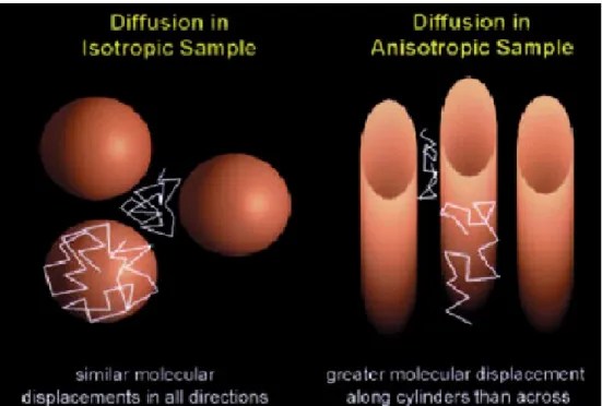
displacements at a molecular level. The DTI protocol highlights the distribution of water molecules (in three dimensions). In a medium with free water motion, the diffusion of water molecules is expected to be isotropic, the same in all directions. With water embedded in nonhomogeneous tissue, motion is expected to be anisotropic, not the same in all directions, and might show preferred directions of mobility. DTI fully characterizes diffusion anisotropy locally in space, thus providing rich detail about tissue microstructure. However, little has been done to define metrics or describe credible statistical methods for analyzing DTI data.
diagnostic approaches like QQ-envelop and SiZer, one can examine whether the
ACKNOWLEDGEMENTS
TABLE OF CONTENTS
LIST OF FIGURES ... vii
LIST OF ABBREVIATIONS ... ix
Chapter I. INTRODUCTION ... 1
Motivation ... 1
DTI Summary Measures ... 3
Wishart Sphericity Tests ... 4
II. NOTATION AND KNOWN RESULTS ... 6
Matrices ... 6
DTI Definitions ... 7
Distribution Theory ... 9
Diffusion Measures in Terms of Wishart Matrices ... 11
First Moment Properties of Eigenvalues (Component Variances) ... 12
Second Moment Properties of Eigenvalues ... 13
Fractional Anisotropy ... 13
Diagnostic Techniques ... 13
Analysis Techniques ... 21
III. APPROXIMATIONS OF THE GEISSER-GREENHOUSE SPHERICITY ESTIMATOR DISTRIBUTION: PAPER 1 ... 24
V. NON-PARAMETRIC ANALYSIS TECHNIQUES FOR DIFFUSION TENSOR
IMAGING DATA: PAPER 3 ... 44
VI. CONCLUSIONS AND FUTURE RESEARCH ... 55
APPENDICES ... 57
LIST OF FIGURES
Figure 1. Diffusion in two types of samples... 2
Figure 2. DTI voxel representations... 4
Figure 3. Illustration of two class discrimination with separating hyperplane... 21
Figure 4. Approximate and simulated densities of when s% %¸0.353 and : œ $... 27
Figure 5. Approximate and simulated densities of when s% %¸0.496 and : œ $... 27
Figure 6. Approximate and simulated densities of when s% %¸0.889 and : œ $... 28
Figure 7. Approximate and simulated densities of when s% %¸0.89 and : œ4... 29
Figure 8. Approximate and simulated densities of when s% %¸0.496 and SNR = 5 ... 30
Figure 9. Approximate and simulated densities of when s% %¸0.889 and SNR = 5 ... 31
Figure 10. Six histograms of the fits of the transformed right cerebellum data... 35
Figure 11. QQ-envelop plot of the subject with the worst fit from Figure 10... 36
Figure 12. QQ-envelop plot of the subject with the best fit from Figure 10... 37
Figure 13. Six histograms of the fits of the transformed corpus callosum data... 38
Figure 14. QQ-envelop plot of the subject with the worst fit from Figure 13... 39
Figure 15. SiZer plot of the subject with the worst fit from Figure 13... 40
Figure 16. QQ-envelop plot of the subject with the best fit from Figure 13... 41
Figure 17. SiZer plot of the subject with the best fit from Figure 13... 43
Figure 18. Raw FA corpus callosum data for all 32 subjects once DWD was performed... 47
Figure 19. Transformed FA corpus callosum data for all 32 subjects once DWD was performed... 48
Figure 20. Transformed FA corpus callosum data for all 32 subjects once DWD was performed on 31 subjects (all but outlier)... 50
Figure 22. DiProPerm results for the transformed FA data of the corpus callosum on all
32 subjects... 53
Figure 23. DiProPerm results for the transformed FA data of the corpus callosum on 31 subjects (all but the outlier)... 54
Figure 24. Approximate and simulated densities of when s% %¸0.496 and SNR = 10... 57
Figure 25. Approximate and simulated densities of when s% %¸0.889 and SNR = 10... 57
Figure 26. Approximate and simulated densities of when s% %¸0.496 and SNR = 15... 58
Figure 27. Approximate and simulated densities of when s% %¸0.889 and SNR = 15 ... 58
Figure 28. Approximate and simulated densities of when s% %¸0.496 and SNR = 20 ... 59
LIST OF ABBREVIATIONS
Abbreviation Meaning
DiProPerm Direction projection permutation DTI Diffusion tensor imaging
DW Diffusion weighted
DWD Distance weighted discrimination FA Fractional anisotropy
HDLSS High dimension low sample size LBI Locally best invariant
1. INTRODUCTION
1.1 MotivationA recent protocol innovation with magnetic resonance imaging (MRI) has resulted in diffusion tensor imaging (DTI). The approach holds tremendous promise for improving our understanding of neural pathways, especially in the brain. MRIs work by recording
displacements at a molecular level. The DTI protocol highlights the distribution of water molecules (in three dimensions). In a medium with free water motion, the diffusion of water molecules is expected to be isotropic, the same in all directions (Figure 1). With water embedded in nonhomogeneous tissue, motion is expected to be anisotropic, not the same in all directions, and might show preferred directions of mobility (Figure 1). DTI characterizes diffusion anisotropy locally in space, thus providing rich detail about tissue microstructure. DTI allows tracking fibers in the brain, a result which has many potential applications. Combining fiber tracking with functional MRI seems likely to elucidate many structure-function relationships. Due to the fact that MRI protocols are noninvasive and are deemed to provide essentially no risk to the participant, longitudinal studies of both diseased and normal participants seem especially promising. DTI has already been used to show subtle
Figure 1. Diffusion in two types of samples. Isotropic (on left) diffusion with similar displacements in all directions and anisotropic (on right) diffusion with greater diffusion in one direction over another (Beaulieu 2002).
Unfortunately, little has been done to define metrics or describe credible statistical methods for analyzing DTI data. Clement (2005) developed a methodological sequence guided by basic principles to help address what measurement should be used to analyze DTI data. It was shown that one-to-one transformations of the fractional anisotropy (FA)
measures lead to accurate representations of their observed distributions in terms of only two estimated parameters each. Using this transformed value will lead to outcomes in statistical models that avoid the “curse of dimensionality” (having far more variables than independent sampling units). Clement also described exact distributional results and a similar analysis for the average diffusion coefficient (ADC).
address whether the approximations are adequate, presenting diagnostic tools for showing if the approximations work on the data, and then discussing new ways of analyzing data if multimodality occurs.
1.2 DTI Summary Measures
With early diffusion MRI techniques, diffusion was described using a single, scalar parameter, the diffusion coefficient, D. However, since diffusion can occur in all three dimensions, it is more fitting to use a diffusion tensor, H. Westin et. al. (1999) showed how to calculate Hand then presented a decomposition of H based on its symmetric properties. Relationships among the eigenvalues of a diffusion tensor classify it according to
geometrically meaningful criteria. Hence Westin et. al. described how to compute the closeness of a diffusion tensor to the generic cases of a line, plane and sphere. In turn, the ratio of the smallest and largest eigenvalues gives a measure of anisotropy, which
corresponds to describing the deviation from the spherical case.
Le Bihan et. al. (2001) took a different approach to extracting information from DTI data. They thought of Has a$ ‚ $ estimated covariance matrix, , at the location ofDs interest. Diffusion data could be analyzed in three ways to provide information on tissue microstructure and architecture for each voxel. 1) The mean diffusivity characterizes the overall mean-squared displacement of molecules and the overall presence of obstacles to diffusion. 2) The degree of anisotropy describes how much the molecular displacements vary in space and how they are related to the presence of oriented structures. 3) The main
Figure 2 represents how DTI data can be viewed. The graphic on the left shows individual voxels ß Hsß represented as ellipsoids; ellipsoids that appear more elliptical are anisotropic, while those that appear spherical are isotropic. The data can then be looked at in
Tensor field
MD map
FA map
Fiber extraction
ß
à
Ä
Figure 2. DTI voxel representations (Gerig et. al. 2006).
many different ways. The first is a MD (mean diffusivity) map (Figure 2 right top), which displays the mean diffusivity of each Hs. The second is an FA (fractional anisotropy) map, which displays the fractional anisotropy measure of each Hs. The third is a fiber extraction map, where fiber bundles in the brain can be depicted.
1.3 Wishart Sphericity Tests
A multivariate Gaussian has a sample covariance following a Wishart distribution (Muller and Stewart, 2006). Later, a one-to-one correspondence with DTI analysis will be shown.
Generally, sphericity corresponds to the statement that all correlations among
quantifying the deviation from sphericity with a parameter that is defined as the square of the trace of the covariance matrix divided by the trace of the squared covariance matrix. Using this definition, the reciprocal sample value is a simple multiple of the locally best invariant (LBI) test statistic for sphericity (John 1972). The likelihood ratio (LR) test statistic for sphericity is a function of the determinant of the covariance matrix over the squared trace of the covariance matrix. Adjusting the formula that Khatri and Srivastava (1971) derived for the exact non-null distribution for the LR test statistic and extending the exact null density function obtained by John (1972) for the LBI test, Sugiura (1995) derived exact formulas for the non-null density function of the LBI and LR tests for testing sphericity in trivariate normal distributions. Power comparisons were also made and Grieve's (1984) conjecture that the LBI test has more power if the population deviation from sphericity is large was
2. NOTATION AND KNOWN RESULTS
2.1 MatricesA vector (a column) is lower case bold, , and a matrix is upper case bold, C H, with transpose Hw. Here, M is an identity matrix, " is an 1 vector of 1's, and Dg B is
8 8 ‚ 8 8 8 ‚
a diagonal matrix with 4ß 4 element B4. The rank of a matrix is the maximum number of linearly independent rows or columns. A square and full rank matrix, , has a unique andE full rank inverse, E". Schott (1997) has details of matrix properties that are not formally given. The trace of H, tr(H), is equal to the sum of the diagonal elements of H and the determinant of H, det(H), will also be denoted as ¸ ¸H . The eigenvalues of H, namely , -are defined as the roots to the characteristic equation ¸H M- ¸œ!. The trace and
determinant of a matrix have simple relationships to the eigenvalues: tr(HÑ œ3œ"8 -3, and ¸ ¸ #H œ 3œ"8 -3.
If H is a symmetric 8 ‚ 8 matrix, there exists an 8 ‚ 8 orthonormal matrix, Z, and an
8 ‚ " vector, , such that - H œ ZDg - Zw, which provides the spectral decomposition. Here, Z Zw œZ Z œ Mw and Dg - is the diagonal matrix of eigenvalues. The columns of Z œc@ á @" 8dare the eigenvectors of H, corresponding to the eigenvalues. The trace and determinant of H are invariant to orthonormal transformations of the form SHSw, for SSw œS Sw .
. - -. -. - -. - - - -" w 5œ" : 5 1 : 5œ" : 5 # 5
w # #
5œ" : # 5œ" 5
: # # #
œ œ Î:
œ
œ œ Î:
œ Î: œ
$ ˆ ‰ (1) (2) (3) (4)
Although expressed here in terms of population constants, the second central moment will be referred to as the variance.
2.2 DTI Definitions
Diffusion tensors are estimated from the raw data contained in diffusion-weighted (DW) images using a relationship between the measured echo attenuation in each voxel and the applied magnetic field gradient sequence. From the following formula, the diffusion tensor is related to the measured echo magnitudes:
(5)
tr
lnEÐ ÑÎE, , œ! œ , H
,H 3œ" 4œ"
$ $
34 34
œ
where E , and A,œ !are the echo magnitudes of the diffusion weighted and non-diffusion weighted signals, respectively, and ,34 is the component of the -matrix, where the, ,-matrix summarized the attenuating effect of all gradient waveforms applied in the , , andB C D directions. Each DW image and its corresponding -matrix is used to estimate , Hs using multivariate linear regression of 5 (Basser and Jones 2002). Thus, each voxel is dependent on the -matrix, which is a function of the diffusion sensitizing gradient strengths and,
duration. Diffusion tensor measurements require that images be acquired with at least six different -value matrices, , ,. A seventh measurement is required with no diffusion weighting to provide a reference measure of signal intensity without a diffusion gradient (E, != ) (Basser and Pierpaoli 1998).
sensitizing field gradient, and the signal intensity in the presence of gradientW is
1œ 1 ß 1 ß 1 B C Dw. The loss of signal intensity due to diffusion is given by the Stejskal-Tanner formula: ln W œ ln W9 # $ ?# # Î$$ 1 H1w , where is the gyromagnetic ratio of H# " (protons), is the duration of the diffusion sensitizing gradient pulses and is the time$ ? between the centers of the two gradient pulses. Using the images, a system of equations is8
used to solve for the unknowns, the 6 elements of the symmetric diffusion tensor, H, and W9 (Westin et. al. 1999).
Zhu et. al. (2007) proposed a semi-parametric model to fit the log-transformed signal intensities in diffusion-weighted MRI data that also characterizes the random noise in the magnitude of the observed signal intensity. If there are DW images for each subject, with8
each image containing R voxels, each of those voxels consists of diffusion-weighted8
measurements. Let W ß3 <3, and be the DW measurements at a single voxel in the human,3 8 brain, where W3 is the signal intensity of the MR image, is a 1<3 ‚3 vector that represents the th direction of the diffusion gradient such that 3 < <3w 3 œ", and is the corresponding ,3 ,
factor of each 3>2 DW MRI (Stejskal and Tanner 1965; Anderson 2001; Kingsley 2006). A weighted least squares (WLS) estimate of the diffusion tensors is then provided from a semi-parametric model. The following heteroscedastic linear model to fit log-transformed signal intensities was considered:
logW œ3 logW ,9 3< H<w3 3!(3 œ D3)!expÐ D3w)Ñ5%3ß where 3 − "ß á ß 8e f, )w
9
is a column vector with logW as its first entry and the six unique elements of Has its other components (in the order: H""ß H"#ß H"$ß H##ß H#$ß H$$), (3 œexpÐD3w)Ñ5%3, and the errors are independent random variables that have mean zero%3 and finite variances. D3 is a 7‚1 vector with the first row equal to 1 and the subsequent rows to be as follows: , < ß #, < < ß #, < < ß , < ß #, < < ß , <3 3ß"# 3 3ß" 3ß# 3 3ß" 3ß$ 3 3ß## 3 3ß# 3ß$ 3 3ß$# . The WLS algorithm for the above model is as follows:
1) Set 5 œ ! and calculate the initial )sÐ5Ñ
3œ" 3œ" 8 " 8
2) Calculate =3 5 œexpŠ#D3w)s5 ‹for all .3
3) Calculate )s5!"using the following equation )
s5!" 3 5 3 5
3œ" 3œ"
8 " 8
3
œ= D D3 3w = D3logW. (6)
4) Repeat steps 2 and 3 for 59 iterations to get the estimate s)Ð5 Ñ9 Þ
This estimate will contain the unique element of Hs, the estimated diffusion tensor (Zhu et. al. 2007).
The DTI variable that is the most useful in analyzing data is fractional anisotropy (Clement 2005). Fractional Anisotropy, , is defined in terms of9
9 -
-. . . . . . # 5œ" $ 5 # 5œ" $ 5 # # "
w w #
# w # "
w w #
# w
œ $
#
œ $ † $
# † $ œ $ # ˆ ‰ ‘ ‘ . (7)
Here is a measure of the dispersion (variance) of the variances of the diffusion tensor (Le9 Bihan et. al. 2001).
2.3 Distribution Theory
Johnson, Kotz and Balakrishnan (1995) and Kotz, Balakrishnan and Johnson (2000) provide detailed properties of the following random variables. Writing F µ" / ‡"ß/‡# indicates that follows a Beta distribution with F /‡"and /‡# as the shape parameters. Writing
\ µ; / =# ß indicates that follows a chi-square distribution, with degrees of freedom\ / and noncentrality . Likewise, writing = V µ J/ / ="ß #ß indicates that follows aV
] ]w W W :
œ µj / ßD ?ß indicates that has a Wishart distribution with degrees of/ freedom, covariance , and D ? œE ]w E ] . Additionally, ] µ E ] ß
ß:
a/ M/ß D
indicates that ] has a matrix Gaussian distribution with mean of E ] , covariance structure of the columns, within a row, of D, and the covariance structure of the rows, within a
column, of M/.
A population or sample covariance matrix is always symmetric and can be expressed as an inner product. The covariance matrix will always have a spectral decomposition with only positive or zero eigenvalues. If E is the matrix of eigenvectors of the covariance matrix,
then Dœ EDg - Ewith E Ew œEEw œM,. Also, if ^ µa/ß,Q^ßM M/ß ,and DœFFwß where FœEDg - "Î#, then ] œ^Fw µa/ß,Q]ßM/ßD with Q œ Q] ^Fw and
] ]w µj,/ß DßQ Q]w ] (8)
(Muller and Stewart 2006).
The locally best invariant (LBI) test for testing sphericity (H! À Dœ5#M:Ñ for unknown 5#, against all alternatives, is to reject the null hypothesis for large values of
Y œtr( W#ÑÎtr W #(John 1971). For this paper, is defined as:% % - -- -- -. .
œ Î :
œ :
œ Î: Î:
œ
œ
tr tr (9)
.
# #
4œ" 4œ"
: :
4 # 4#
4œ" 4œ"
: :
4 # 4#
# # " w #
# w
ˆ ‰‘
ˆ ‰ ˆ‚ ‰ ˆ ‰ ˆ‚ ‰ ˆ ‰
D D
Thus, the maximum likelihood estimate (MLE), , of the parameter is a one-to-one functions% % of the LBI test for sphericity, s œ "Î :Y% .
When : œ $, which is the case in diffusion tensors, the exact density function of Y
, Ð?Ñ œ - ÖÒ&*?! #Ð$?"Ñ Ó Ò&*? #Ð$?"Ñ Ó × Ÿ ? Ÿ
- ÖÒ&*?! #Ð$?"Ñ Ó × 8 ? Ÿ "
Y
$Î# Î#" $Î# Î#" " "
$ #
$Î# Î#" "
#
/ ÈÈ È
/ /
/ / ,
(10)
with - œ/ È 1> /$ Î# Î ˜> / Î# c#> / " Î# &% d "Î#™ where > B œ B " x where is aB
positive integer.
Let
1 ÐBß ?Ñ œ $ Î# B B ! B ‚
Î# "Î# #Î# #
" ?
" ?
# #B ! $B
! # $ Î## # È Œ Œ 1> / > / > / > /
/
(11)
and
1 ÐBß ?Ñ œ $ Î# ‚
5x # Ò" ! ! # BÓ
#5 ! " x #5 xG E G \ #5 #5 ! " $Î# 5 x
" " # Î# 5œ!
∞ 5
# $5 5!$ Î#
" # " " " #
" # 5 #
# # / # # / / , , , " (12)
with #3 œ- -3Î $, + 5 œ +Ð+ ! "Ñá Ð+ ! 5 "Ñ +, ! œ "ß E œDg" "Î ß " "Î#" ##,
\ œDgŠ" $B !È#? $B ! #B "ß " $B # È#? $B ! #B "# ‹. Here , stands for the sum of all possible partitions , œ Ö5 ß 5 ×" # of non-negative integer satisfying5 5 œ 5 ! 5" #and 5 5 !" # . Also, G, † is the zonal polynomial corresponding to the
partition . Then the non-null density of is, Y
0 Ð?Ñ œ 1 ÐBß ?Ñ ‚ 1 ÐBß ?Ñ .Bß Ÿ ? Ÿ
1 ÐBß ?Ñ ‚ 1 ÐBß ?Ñ.Bß 8 ? Ÿ "
Y "Î$ # $?" Î$ "Î$ # $?" Î'
! " "$ "# !
"Î$ # $?" Î'
! " "# Ú
Û Ü ' '
È È È
,
(13)
Although the density exists, it involves zonal polynomials, which seems likely to cause problems with computation.
2.4 Diffusion Measures in Terms of Wishart Matrices
diffusion. In other words, D will indicate the population covariance of diffusion. As a consequence of the assumption, /Ds µj /: ßD (follows a Wishart distribution) with / being determined by the number of replicates used to find Ds and equaling the number of:
rows in . The eigenvalues of , Ds Ds š ›-s3 , are estimates of variances of underlying principal components and hence measures of diffusion in orthogonal dimensions. The most popular measures of diffusion arising from DTI analysis can be expressed solely as functions of the sample eigenvalues which are, in fact, estimated variances.
2.5 First Moment Properties of Eigenvalues (Component Variances)
Trace and ADC. Interpreting the eigenvalues, e f-3 , as measures of variance, then ."w is the average variance, or the arithmetic mean of the variances. When W œ/Ds is a Wishart,
:"trŠ ‹Ds is often called the generalized variance. Johnson, Kotz and Balakrishnan (2000) expressed the trace of a singular covariance matrix with degrees of freedom less than its dimension in terms of a weighted sum of chi-square random variables. Glueck and Muller (1998) derived that the trace of a Wishart equals a weighted sum of noncentral chi-square random variables and constants. The average diffusion coefficient (ADC) is the trace of the tensor, hence it is exactly distributed as a weighted sum of central chi-square random variables (Glueck and Muller 1998). The exact distribution of the ADC can always be computed. An approximate and highly reliable distribution is also available. Kim, Gribbin, Muller, and Taylor (2005) provide a convenient review of exact and approximate calculations of probabilities for such quadratic forms.
Determinant. If e f-3 are thought of as measures of principal variation, then
.1 œˆ ‰.:1 "Î: is the geometric mean of the variances. The sample generalized variance can also be defined as ¹ ¹Ds . Although it is common in statistics to discuss ¹ ¹Ds as the generalized variance, it seems more natural to look at the geometric mean, .s œ1 Ê ¹ ¹: Ds . Gupta and Nagar (2000, Chapter 3) showed the following. If W µ j /: ß , Î µ ?3, with
independent e f.3 and 3 ;# , where e f. Also, 3!"
? µ / 3 − "ß á ß :
IŠk kW 2‹œ #:2k k2# e cÐ"Î#ÑÐ 3 ! "Ñ ! 2 Îdf e cÐ"Î#Ñ 3 ! "df
3œ" :
D > / > / .
2.6 Second Moment Properties of Eigenvalues
In order to achieve global scale invariance, the measures of dispersion of diffusion (anisotropy) are standardized; thus the central information will remain unchanged if a linear transformation is applied. The main goal is to see if the variances are the same in all three dimensions. By using the parameter estimates š ›-s3 , estimates for can be obtained. Box% (1954) showed was a function of sphericity; thus, a one-to-one function of provides the% % locally best invariant test for sphericity by 9 . Using this information, FA can be expressed as one-to-one functions of , the LBI test statistic for sphericity.s%
2.7 Fractional Anisotropy, 9
By Equation 7,
9 . .
. %
# #w "w # # w
œ $ † $
# † $
œ $ " #
‘
.
(14)
Hence 9s#is scale invariant and
% 9
s œ " # $s
#
. (15)
Thus, a linear function of 9s# is a one-to-one function of a LBI test for sphericity (Clement 2005). The LBI test for sphericity will be more powerful with values of near one (Sugiura% 1995). Experience with DTI brain data shows that the values of fit this case. We wills% show that can be approximated by a squared beta distribution. Thus, FA can bes% approximated by a squared beta distribution.
2.8.1 Kernel Density Estimation
The histogram is a widely used tool for displaying the distributional shape of a set of data. Its usefulness lies in the fact that it indicates the shape of the underlying density function. An alternative to estimate the density function is a smooth curve. In order to discuss the construction of estimators of this type, it is important to first consider the construction of a histogram. However, when viewed as an estimate, the histogram can be criticized in the following ways: 1) information is thrown away when the observed values are replaced by a central point in the interval in which they fall; 2) the underlying density
function is usually assumed to be smooth, but the estimator is not smooth, due to sharp edges of the boxes from which it is built; and 3) the behavior of the estimator is dependent on the choice of width of the intervals used, and also to some extent, on the starting position of the grid of intervals (Bowman and Azzalini 1997, Chapter 1).
Whittle (1958) and Parzen (1962) developed an approach to the problem which removes the first two of these issues. A smooth kernel function, rather than a box, is used as the basic building block. These smooth functions are centered directly over each observation. The kernel estimator is then of the form:
0 ÐCÑ œ "Î8 AÐC C à 2Ñß
s
3œ" 8
3 (16)
where is a probability density called the A kernel function, whose variance is controlled by the parameter . Because of its role in determining the way in which the probability2
associated with each observation is spread over the surrounding sample space, is called the2
smoothing parameter or bandwidth. Since properties of are inherited by A s0, choosing toA
be smooth will produce a density estimate which is also smooth.
The basic properties of are well documented (Bowman and Azzalini 1997, Chapter 2).s0
The mean of the density estimator can be written as
This is a convolution of the true density function with the kernel function . Smoothing hasA
thus produced a biased estimator, whose mean is a smoothed version of the true density. Using a Taylor series approximation argument, we can approximate the expected value
I 0 ÐCÑ ¸ 0 ÐCÑ ! Ð2 Î#ÑŠs ‹ # 5A#0 ÐCÑßww (18) where 5A# denotes the variance of the kernel function, namely 'D AÐDÑ.D# . Since 0 ÐCÑww
measures the rate of curvature of the density function, this expresses the fact that s0
underestimates at peaks and overestimates troughs in the true density. The size of the bias0
is affected by the smoothing parameter .2
Through another Taylor series approximation, the variance of the density estimate can be approximated by
@+< 0 ÐCÑ ¸ Ð"Î82Ñ0 ÐCÑ ÐAÑߊs ‹ α (19) where αÐAÑ œ 'A ÐDÑ.D# . Note that the variance is inversely proportional to sample size. The term 82 can be viewed as governing the local sample size, since controls the number2
of observations whose kernel weight contributes to the estimate at . It is also noteworthyC
that the variance is approximately proportional to the height of the true density function.
These approximate expressions for the mean and variance of a density estimate encapsulate the effects of the smoothing parameter. As decreases, bias diminishes while2
variance increases. As increases, the opposite occurs. The combined effect being that in2
order to produce an estimator which converges to the true density function, it is necessary that both and 2 "Î82 decrease as the sample size increases.
It must also be noted the third criticism of the histogram still applies to the smooth density estimate, namely that its behavior is affected by the choice of the width of the kernel function. When is small, the estimate displays the variation associated with individual2
observations rather than the underlying structure of the whole sample. When is large, this2
Optimal Smoothing
An overall measure of the effectiveness of s0 is provided by the mean integrated squared
error (MISE). The MISE can be defined as
MISEÐs œ I s .C (20)
œ I 0 ÐCÑ .C ! @+< .CÞ
0 Ñ 0 ÐCÑ 0 ÐCÑ
0 ÐCÑ 0 ÐCÑ
s s
œ( ’ “
( ’ š › “ ( š › #
#
and can be approximated by
MISEŠ ‹s0 ¸ Ð"Î%Ñ2% %5A( 0 ÐCÑ .C ! Ð"Î82Ñ ÐAÑÞww # α (21)
From this approximate expression, the value of which minimizes MISE is2
2opt œ e#ÐAÑÎÐ Ð0 Ñ8Ñ" f"Î&ß (22)
where #ÐAÑ œ ÐAÑÎα 5A%, and "Ð0 Ñ œ 0 ÐCÑ .CÞ' ww # However, this optimal value for cannot2
immediately be used in practice since it involves the unknown density function, but it is informative in showing how smoothing parameters should decrease with sample size and in quantifying the effect of the curvature of through the factor 0 "Ð0 Ñ.
Normal Optimal Smoothing
If it is assumed that is a normal distribution, the following simple formula for 0 2opt
arises:
2opt œ 5%Î$8"Î&ß (23)
where denotes the standard deviation of the distribution. For distributions not far from the5 normal, this gives a useful choice of smoothing parameter that requires very little calculation. With this, it also has the potential for being cautious and conservative.
Cross-validation
approach, labeled as cross-validation. Stone (1974) gives a general description of the ideas involved in validation. It must be noted that there are distinctions between cross-validation and data splitting. As Picard and Cook (1984) cautioned, "Implementation of cross-validation in the derivation of does not, however, alter the fundamentals of predictive"s assessment. If a proper evaluation of a selected fitted model is to be realized, the optimism principle cannot be ignored. When using data splitting, this implies that all aspects of model selection (even those that are crossvalidatory) should be confined to analysis of the
estimation data and that the validation data be reserved solely for assessment." Thus, the use of the phrase "cross-validation" in this sense is synonymous with a "leaving -out" approach.5
It should be noted that is not a way to validate a model, but is a way to select a model.
Rudemo (1982) and Bowman (1984) applied cross-validation ideas to the problem of bandwidth choice through estimation of the integrated squared error (ISE)
( šs0 ÐCÑ 0 ÐCÑ›#.C œ ( 0 ÐCÑ .C # 0 ÐCÑ 0 ÐCÑ.C !s # ( s ( 0 ÐCÑ .C# Þ (24)
Note that the last term on the right hand side of the equation does not involve ; thus this2
term can be ignored in the minimization. The second term on the right hand side of the equation can be split into two terms, one involving and the other not (Bowman 1984). The2
terms that involve can be estimated by the following formula:2
Ð"Î8Ñ( s s ß
3œ" 8
0 ÐCÑ.C Ð#Î8Ñ#3 0 ÐC Ñ
3œ" 8
3 3
(25)
where s0 ÐC Ñ3 3 denotes the estimator constructed from the data without the observation C3 (Bowman and Azzalini 1997, Chapter 2). The expectation of this expression is the MISE of
0 8 " 0 2
s based on observations, omitting the ' # term. The value of which minimizes this expression therefore provides an estimate of the optimal smoothing parameter.
Plug-in Bandwidth
"Ðs0 Ñ can be calculated relatively easily and the value of which solves this equation can be2
found by a suitable numerical algorithm.
Sheather and Jones (1991), extending the work of Park and Marron (1990), described a bandwidth selection procedure based on the estimation of 0ww using an additional smoothing parameter related to . This estimator has very good finite sample, as well as asymptotic,2
properties. It is more stable than the cross-validation approach described above. The two techniques take separate approaches to the same problem of minimizing ISE. Cross-validation estimates the ISE function and locates the minimum. The plug-in approach minimizes the function theoretically and then estimates this minimizing value directly.
2.8.2 Exploratory Tool
When analyzing data using smoothing methods, it is difficult to determine whether peaks and valleys are important underlying structures or artifacts of the sampling process. Since both of these can be made to disappear by increasing the amount of smoothing or can increase the number of features if the smoothing parameter is decreased, it is hard to
determine which of these is true. SiZer (based on studying statistical SIgnificance of ZERo crossings of derivatives) is an exploratory data analysis tool that works in conjunction with smoothing methods to analyze which visible features represent important underlying structures.
Developed by Chaudhuri and Marron (1998), SiZer can be used for both density
estimation (smoothed histograms) and for nonparametric regression (scatter plot smoothing). SiZer investigates which of the features seen in smooths are statistically significant by studying derivatives of the smooths. There are two components to SiZer: 1) use of a family of smooths for a broad range of and 2) a color map of scale space. By using a family2
Scale-space ideas are used to provide a new view on kernel smoothing. The family of all kernel smooths indexed by bandwidth, , is a model used in computer vision. The idea2
behind this is that large models give a macroscopic view where only large-scale features2
can be resolved; whereas, small models give a microscopic view of the small-scale2
features. It is important to choose a range of that highlights a good data based choice.2
Marron and Chaudhuri (1998) suggest the following defaults: evaluate the smooths at a grid of 401 equally spaced points with the smallest equal to twice the grid spacing and the2
largest equal to the range.2
The SiZer map is created based on confidence limits for the derivative in scale space,
0 ÐBÑ2w . These confidence limits are of the form
s0 ÐBÑ „ ;SD sÐ 0 ÐBÑÑßs (26)
w w
2 2
where is an appropriate quantile and the standard deviation is estimated using the following;
definition of the variance.
var sÐ 0 ÐBÑÑ œ 8s = O ÐB \ Ñß á ß O ÐB \ Ñ ß (27)
w
2 " # 2w " 2w 8
where is the usual sample variance of numbers and =# 8 Ow is the -rescaling of the kernel2
2
function Ow, such that Ow † œ "Î2 O † Î2 . An ÐBß 2Ñ location is called significantly
2
increasing, decreasing, or not significant when 0 is below, above or within these confidence limits, respectively. This information is displayed in the second component, a color map of scale space where each pixel represents a location with respect to both position, , andB
bandwidth, . A blue color (or dark if in black and white) is used on the pixel of the color2
map if the smooth is significantly increasing. If the smooth is significantly decreasing, the pixel is colored red (or light) If there is not a statistically significant slope, the pixel isÞ
significant curvature, the pixel is shaded green. This gives an additional look at the data. The SiZer map has two important benefits. First, it speeds up the process of deciding "which features are really there" for an experienced analyst while also being able to quantitatively resolve any "gray area" problems. Second, it allows inexperienced analysts to make inferences about which features are really there (Chaudhuri and Marron 1999).
2.8.3 Q-Q plots
Quantile-quantile (Q-Q) plots are used to compare two distributions. These could be both datasets, both theoretical distributions, or most commonly, a combination of the two. The Q-Q plot is a scatterplot of quantiles of one distribution on each axis, which thus gives direct comparison of the distribution. If the points roughly lie on a plot with slope 1, then the distributions are the same. However, how does one know if values away from the line with slope one are due to variation of the sample or if the data really does not come from the given distribution?
Programs supplied by Marron (2007) delved into an approach called QQ-envelop to use a Q-Q plot to test the distributional form against standard distributions. This method creates a typical Q-Q plot, but then simulates pseudo sets of data from the assumed distribution to look at random variability. All pseudo data points, as well as the original observations, are plotted. If the original data points are enveloped by the pseudo data points and the line with a slope of 1, then the distributional fit works; if not, then the distributional assumption was not correct. This approach was used in Hernandez-Campos et. al. (2004) to fit distributions to' Internet traffic data. Mihee Lee extended the program written by Marron to do this analysis with beta distributions.
2.9 Analysis Techniques
High dimension low sample size (HDLSS) data is becoming increasingly common in
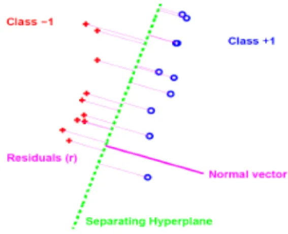
by finding the hyperplane which best separates populations. The distance between the discriminating hyperplane and the data points must be maximized while also separating the two classes. Figure 3 shows a representation of how this can be done. Let be the given:3 points from the - −3 e "ß "fclasses, and be the normal vector to the separatingA
hyperplane. The residual, or distance, is from the points to the hyperplane, can be<3
Figure 3. Illustration of two class (pluses and circles) discrimination with separating hyperplane (dotted line)
Gorczowski e
( t. al. 2007).
calculated by the following function where determines the position of the hyperplane."
< œ - : A !3 3 3w " (28)
2.9.1 Distance Weighted Discrimination
DWD is a multivariate analysis tool that is able to identify systematic biases present in separate data sets and then make a global adjustment to compensate for them (Benito 2004). DWD is also a classification tool described by Marron, Todd, and Ahn (2007). The method starts by dividing the sample union into two classes by a hyperplane and then classifying this combined set as coming from one of the two populations according to whether a point lies on one side or the other of the hyperplane. DWD differs from SVM in how the hyperplane is selected. Unlike SVM, all the sample points are used in the calculation of the discriminating axis. Also, instead of trying to maximize the minimum , DWD attempts to minimize the<3 sum of the reciprocals of . Thus, DWD achieves a higher robustness when presented with<3 new samples since each point's contribution to the calculation was weighted proportionally to the distance from that point to the opposite population (Marron, Todd, and Ahn 2007). Hall et. al. (2005) developed asymptotic properties in the limit as . Ä ∞, of SVM and DWD.
2.9.2 DiProPerm Test
If one wants to know if two subpopulations are from the same distribution, the DiProPerm test (Wichers et. al. 2006) can be used. This is very useful in our imaging scenario because one can see if the brain structure in one group is different from another. DiProPerm (Direction Projection Permutation) uses the following ideas to test if distributions are the same:
1) find an appropriate one-dimensional direction vector where the normal hyperplane
effectively separates the populations;
2) project data into that one-dimensional subspace;
3) construct a one-dimensional test statistic;
4) for many permutations of class labels, repeat the first three steps;
permutation statistics.
First, DWD is performed in order to separate the data groups. Other reasonable
3. APPROXIMATIONS OF THE GEISSER-GREENHOUSE
SPHERICITY
ESTIMATOR DISTRIBUTION
: PAPER 1
Approximately matching the first two moments of to a squared beta random variables% results in a simple approximate distribution. The fact that "Î: Ÿ Ÿ "s% allows concluding
! Ÿ s " " " Ÿ "
: :
Œ% Œ "
. (29)
This leads to defining
F œ s " " "
: :
œs : "
: " : " œ - -s
#
"
" !
Œ Œ Œ Œ
%
%
% .
(30)
Obviously XF œ -# "X%s -! and X%s œ XF ! - Î-# ! ". With X œ" tr#Ð Ñs and X œ Ð# tr s Ñ,
#
D D
it follows that s œ X Î :X% " #. While it is known that the following assumptions are not true,
they were assumed to derive the approximate results. First, it was assumed that X"and X# are
independent. Second, it is assumed that XX#" œXX#". Muller, Edwards, Simpson and
Taylor (2007 reported) that X X" œ # /5œ" ! Ð5œ" 5Ñ X X# œ
: :
5
# # #
/
/ - / - and
/ // /! #:5 œ"" -5#" ! #//:5 œ#" 5 "5 œ"#" - -5 5
" # . Also, from 30 , it is known that
F œ X :X# :Î : " "Î : " F : " ! " œ X ÎX#
" # " #
/ c d c d; thus, .
The special case of sphericity leads to X" being exactly the square of a scaled, central
chi-square. In general, F µw " / ‡"Î#ß/‡#Î# is true if and only if F œ \ Î \ ! \w " " #, with
\"independent of \# and both distributed chi-square. It seems reasonable to find
X% X X
X
s œ F ! -
Î-¸ F ! " Î :
: " : "
¸ : " F ! "
: :
ˆ ‰
” Œ • Œ Œ Œ
#
! " ‡#
‡# .
(31)
Moments of a Beta are described in Johnson, Kotz, and Balakrishnan (1995, Chapter 25). Thus, for such a F‡,
F œ \
\ ! \
œ \
\ ! # \ \ ! \
#
‡ ‡" " # # ‡" " ‡# # #
‡" " # #
‡" " ‡# #
# # # #
‡" ‡# " # -- -- - - , (32) with
X X X X X
- / / - - / / - / /
ˆ ‰
\ ! #\ \ ! \ œ \ ! # \ \ ! \
œ ! # ! # ! ! #
" # " #
# # # #
" # " #
# #
‡" ‡" ‡" ‡" ‡# ‡" ‡# ‡# ‡# ‡# . (33)
As a Beta random variable, XF œ# / / ! " / !/ / !/ ! " . Hence, by ‡ ‡" ‡" c ‡" ‡# ‡" ‡# d"
taking the expectation of the numerator and denominator separately,
X% / /
/ / / /
s ¸ : " ! " ! "
: ! ! ! " :
Œ ‡"‡" Œ ‡" ‡# ‡" ‡#
. (34)
Similarly, as a Beta random variable,
X / / / /
/ / / / / / / /
F œ ! " ! # ! $ Þ
! ! ! " ! ! # ! ! $
% ‡
‡" ‡" ‡" ‡"
‡" ‡# ‡" ‡# ‡" ‡# ‡" ‡#
(35)
Hence, by treating the numerator and denominator separately,
VarÐ Ñ ¸s : " # ! " # ! # ! ' ! $ ! $
: ! ! ! " ! ! # ! ! $
% / / / / / / / /
/ / / / / / / /
Œ
#
‡" ‡# ‡" ‡"# ‡" ‡# ‡" ‡# ‡" ‡# # ‡" ‡# # ‡" ‡# ‡" ‡#
. (36)
Without the : " Î: term, this would be what one would expect for the variance of a squared beta distribution. Thus, the approximation depends on such that: as increases,:
the approximation gets better and better since : " Î: Ä " as : Ä ∞.
one million replications. Using a known epsilon, random Wishart matrices were generated by first creating random normal matrices. A random number generator produced matrices to create a matrix. The random number generator used normal values with mean zero and^ variance of 1. Since epsilon is a function of eigenvalues, H1 - was created to achieve the epsilon of choice. ] was set equal to ^EH1 - "Î#. Since D in this case would be
F Fw œ H1 - w"Î#E Ew H1 - "Î# E F Fw œ H1 - H1 and is orthonormal, . Hence only and ^ are required to produce the Wishart matrices. The following entries comprised the matrix, H1 - : 1.00, 0.02, 0.01 for an %œ0.353, 0.80, 0.09, 0.10 for % œ0.496 and 1.00 0, .55, .55 , fo0 r %œ0.889. By 8 , ] ]w was the resulting random Wishart matrix. For each ] ]w , was then computed. These values were then transformed into valuess% F using the square root of 30 . The distribution of the transformed values as well as the corresponding beta distribution were plotted. As increased, the fit became even better,:
which is logical since both the mean and variance are dependent on a function of . It must:
be noted that in a DTI setting : œ $; however, the use of : L $ is shown to demonstrate a more general use of this finding.
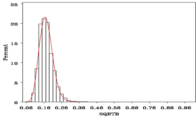
Figures 4 5 and 6 show the accuracy of the approximations when ß ß : œ $. The solid red line represents the approximations based on a Beta random variable, while the histogram is from the sample values from the simulation described above. Figure 4 summarizes the simulation when %¸ 0.353. Since so many replicates were used, using a p-value for a goodness of fit test does not make sense since it is dependent on the sample size. If one were used, the fit would need to be perfect in order to get a non-significant result. However, the Kolmogorov-Smirnov test statistic, H œmax¹J B Js obs B ¹ was calculated. Because H already denotes the diffusion tensor, the Kolmogorov-Smirnov test will be given as OW for the rest of the paper. Note that this statistic is bounded by and with a perfect fit = and! " !
Figure 4. Approximate (red) and simulated (black) densities of
when 0.353 and ( 5 .
% %
s
¸ : œ $ OW œ !Þ! !$*$Ñ
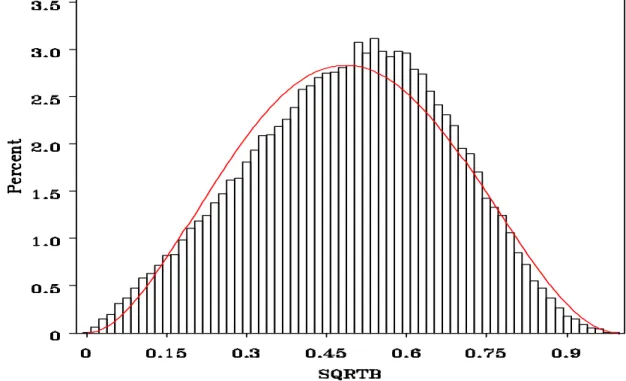
Figure 5. Approximate (red) and simulated (black) densities of
when 0.496 and ( .
% %
s
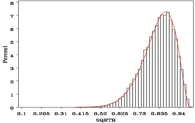
Figure 5 summarizes the simulation when %¸0.496. In Figure 5, the fit works reasonably well, but is not perfect OW œ !Þ!%%&). It is good to note that the LBI test is more powerful for large values of , hence we would expect better fits as % % Ä ".
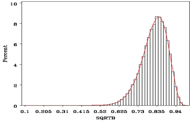
Figure 6 summarizes the simulation when % ¸0.889. The figure shows that this distribution works extremely well for larger values of epsilon OW œ !Þ!"!'#(. This again was expected, as the LBI test is the better test for large epsilon. Remember that Figures 5 and 6 are for the case where : œ $, or a $ $× matrix. The fits will only improve as increases.:
To show this, a simulation was performed when : œ %. Figure 7 shows when %¸ !Þ)* and
: œ %. Note that the fit still works extremely well, if not better, since the overlayed beta
distribution has a better fit near the apex of the curveOW œ !Þ!!&'%&*.
Figure 6. Approximate (red) and simulated (black) densities of
when 0.889 and ).
% %
s
Figure 7. Approximate (red) and simulated (black) densities of
when 0.89 and .
% %
s ¸ : œ % OW œ !Þ!!&'%&*
However, when dealing with DTI data, random noise must be accounted for. Thus, an additional simulation was performed that created random Hs by using the WLS algorithm in
6 with "!!ß !!! replicates. Simulated diffusion-weighted images were generated as follows: W9 was fixed at "&!!, values of 59 were varied to provide differing signal-to-noise ratios (SNR = W Î9 59) of 5, 10, 15, 20, 25 and 30. Similar to the simulations in the Zhu et. al. (2007) paper, an imaging acquisition scheme e, ß < À 3 œ "ß ÞÞÞß $!3 3 f was used that consists of 7 œ & baseline images with , œ ! s/mm and # 8 7 œ #& directions of diffusion gradient at , œ "!!!s/mm and equivalent to the matrix provided in the Hardin (1994)# <3 web site when 7 œ $!. For a given diffusion tensor, , , and were generated from aH B3 C3
simulations above, was defined with the diagonal elements being as follows (units:H "!$mm/s): 0.80, 0.09, 0.1 , for an % = 0.496 and 1.00, 0.55, 0.55 , for an =0.889.%
Finally, the resulting 3>2acquisition of the resulting diffusion-weighted data was calculated by
W œ3 W9 ,3 3w 3 ! B3 ! C3 s s
# #
É exp < H< . The were then calculated for each % H computed by the WLS algorithm in 6 with 5 œ &. Similar to the first simulation, the values weres% then transformed into values using the square root of 30 and plotted. The distribution ofF
the transformed values as well as the corresponding beta distribution were plotted.
Figure 8. Approximate (red) and simulated (black) densities of
when 0.496 and SNR = 5 .
% %
s
¸ OW œ !Þ!#*")$
results from the first simulation. If anything, these fits could be slightly better. A main reason why the addition of the noise did not hinder the fits was because the noise that was added was Gaussian, and Beta random variables can be expressed as functions of chi-squared's, which are functions of Gaussians.
Figure 9 summarizes the simulation when % ¸0.889. The figure shows that this distribution works well for larger values of epsilon OW œ !Þ!"(&("*. The reason for the
Figure 9. Approximate (red) and simulated (black) densities of
when 0.889 and SNR = .
% %
s ¸ & OW œ !Þ!"(&("*
fit not being as good as Figure 6 is that this simulation was with SNR = 5, which means a larger 59 used to define and . As the SNR increases, the fits become better; these imagesB3 C3 can be found in Appendix A.
Thus, it has been shown that %s can be approximated by a beta-squared random variable
4. DIAGNOSTIC TECHNIQUES FOR DIFFUSION TENSOR
IMAGING DATA: PAPER 2
The DTI variable that is the most useful in analyzing data is fractional anisotropy (FA) (Clement 2005). FA values are a measure of the deviance from sphericity. Sphericity, or isotropy, of the principal variables, holds if%œ1 (and hence all population eigenvalues are equal). This condition represents the event of water molecules dispersing, or diffusing, uniformly over a given space.
By 7 and 9 ,
9 . .
. %
# #w "w # # w
œ $ † $
# † $
œ $ " #
‘
.
(37)
Hence 9s#is invariant and
% 9
s œ " # $s
#
. (38)
Thus, as FA increases, decreases, and diffusion becomes more anisotropic. Additionally, its%
is shown that a linear function of 9s# is a one-to-one function of the LBI test for sphericity
(Clement 2005). The LBI test for sphericity is more powerful when values of are near one%
(Sugiura 1995). Experience with DTI brain data shows that this is the case. Paper 1 showed
that can be approximated by a squared beta distributions% , with the approximation best at
highest (and lowest) values. Thus, transformed FA values can be approximated by a squared
beta distribution.
There is one main concern of the analysis approach used above. This is that distinct
types of data could be mixed together, especially white and gray matter. Such mixing could
interest, or different segments along a fiber tract. The goal here centers on evaluating how well the beta approximations fit. The recommended approach also was chosen to provide self-diagnostic information quickly about any problems with regions of interest definitions.
In 1987, Box and Draper wrote: "Essentially, all models are wrong, but some are useful." The parametric approach to analyzing diffusion tensor data shows a usefulness for these approximate distributions. It is useful to determine when the approximations are not drastically off base.
The UNC Neurodevelopmental Disorders Research Center provided data for 32
developmentally delayed and typical children. All scans were acquired on a 1.5T GE Sigma Advantage MR scanner. DTI images were acquired using 4 repetitions of 12-direction spin-echo single-shot spin-echo planar imaging (EPI) sequence with a 128x128x130 image matrix at 1.875mm x 1.875mm x 3.8mm resolution with a 0.4mm gap using a -value of 1000 s/mm ., #
Using a custom program designed to automatically remove slices that fall outside
predetermined parameters, each DTI slice was screened for motion and other artifacts. After cleaning, both correction of eddy-current based image distortions using mutual information based unwarping and the calculation of the diffusion tensor elements were performed using another custom software package (Cascio et al. 2008). The resulting eigenvalues and eigenvectors of each diffusion tensor were also calculated and FA values were computed. The FA values from different regions of the brain were transformed into values from 30F . The distribution of the transformed values as well as the corresponding approximating beta distribution were plotted. Diagnostic tests were used to see how the fits were performing. The data is ordered from smallest to largest for each subject. Having the ordered data allowed for simple computation of the empirical quantile function to be used, where the Ci
values are equal to the raw FA values and the values are equal to B3 3Î 8 " , where is8
data to see how the fit relates to other samples from the same beta distribution; also, since multimodality could be an issue, SiZer was also used.
The right cerebellum is a structure located between the cerebrum and the brainstem which is the unit of motor control. There are 453 voxels that make up this region. Figure 10 depicts a sample of fits of the transformed right cerebellum data, with the -axis being theC
percent of data points and the -axis, the value. All of these fits seem to work well;B F
however, we will still look at the diagnostic tests.
%
Beta Value
Figure 10. Six histograms of the fits of the transformed right cerebellum data; actual values (black) and approximate beta distribution (red).
In QQ-envelop, the data are plotted on the y-axis and the values from the assumed distribution are plotted on the x-axis. The red bold line is the Beta Q-Q plot for the
resampling the exact beta distribution. If the results fit, then the red line will be encompassed by the blue lines.
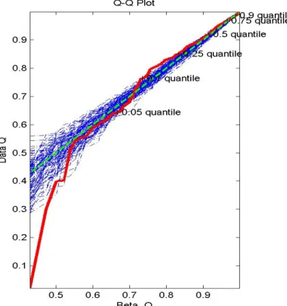
Figures 11 and 12 show the worst and best fits from Figure 10, respectively. One will note that the Q-Q plot for the transformed FA data (red line) in the QQ-envelop plots can deviate quite a bit from the theoretical beta distribution (green line) and is not always encompassed in the 1000 resamplings of the beta distributions (blue lines). In Figure 11, it appears that the data in the lower 5 percentile deviates from the estimated distribution. In>2
Figure 11. QQ-envelop plot of the subject (ID = ) with the worst fit from Figure 10 (plot on third row, second colu
&"&!!!%!#
Figure 12, the red line is encompassed by the blue lines at all points except a small region between 0.6 and 0.65 on the y-axis. SiZer was considered, but will not be shown here because there were no occurrences of multimodality.
Thus, the beta distribution approximation works well in the best case, less well for other subjects in the right cerebellum region of interest. However, if we go back to Box and Draper's statement about modeling, this information is definitely still informative. These fits for the right cerebellum appear to work well enough to be used in analyses, as the fit did work for all but a small fraction of the data, mainly the left tail.
Figure 12. QQ-envelop plot of the subject (ID ) with the best fit from Figure 10 (plot on second row, second column)
œ &"%*!!$!#
. Q-Q plot for the data (red lines), Q-Q plot for the theoretical distribution (green), and Q-Q plot for the resampled
data are displayed. region between 0.60
and 0.65 on the -axis.
The corpus callosum is a region of the brain where this is not the case. The corpus callosum is the largest connective pathway in a human brain that allows the two hemispheres of the brain to communicate with each other. Upon first inspection of the data, the fits did not work well at all. In order to understand why these fits were not working, meetings with the investigators of the study and the DTI team were held. It was agreed that a scientific reason could be that partial voluming (including multiple regions in a voxel) was occurring. This was plausible, especially due to the size of the corpus callosum, and could have caused a bimodal effect in the data. The definition of the region of interest was further investigated and updated. The analysis provided below was performed on the new definition of the corpus callosum region. This region is comprised of 857 voxels.
%
Beta Value
Figure 13 shows the transformed corpus callosum data from six arbitrarily selected children. The fits are obviously not as good as those of the right cerebellum and might even indicate a bimodal distribution. To understand how good the fits were, QQ-envelop was performed. Figures 14 and 16 show the results of the best and worst subjects from Figure 13.
Figure 14 shows that the beta approximation is not working in the first 10>2percentile as well as between the 25 and 50 percentiles for the worst fit from the sample of 6 subjects.>2 >2 This is a worse fit than seen in the right cerebellum data. In order to see if this was the case, SiZer was used.
Figure 14. QQ-envelop plot of the subject (ID ) with the worst fit from Figure 13 (plot on second row, second colum
œ &"&'!!%!#
n). Q-Q plot for the data (red lines), Q-Q plot for the theoretical distribution (green), and Q-Q plot for the resampled data are displayed. The fits do not work well for the first
percentile and between the and percentiles.
"! #& &!
Figure 15 displays the SiZer plot for the same subject displayed in Figure 14. The first plot shows the overlay of the family of bandwidth values used, with the optimal value2
denoted as the bolded black line. The green dots represent each transformed value from each voxel in the corpus callosum region. The horizontal dashed lines represent the percentiles that are plotted in Figure 14. We can see from the family overlay plot that a beta distribution is not likely and that an extra mode could be occurring between the 10 and 25 percentiles.>2 >2
Figure 15. SiZer plot of the subject (ID ) with the worst fit from Figure 13 (plot on second row, second column).
œ &"&'!!%!#
The first graphic is the plot of the family of bandwidths, the second is the slope SiZer map, and the thrid is the curvature SiZer map. From these plots, there does not seem to be any significant results for bimodality.
the smooth is significantly increasing. If the smooth is significantly decreasing, the pixel is colored red, and if there is not a statistically significant slope, the pixel is shaded purple. The black horizontal line denotes the same bandwidth that corresponds to the bolded black curve in the family bandwidth plot. Up until the peak between the 10 and 25 percentiles, the>2 >2 curve is increasing, but doesn't show a decreasing slope until around the 90 percentile.>2 Thus, significant bimodality is not shown even though there are separate modes in the first graphic of Figure 15. However, the dark black line in the first graphic in Figure 15, does not depict what one would expect from a probability density function of a beta distribution, as the pdf of a beta distribution would be an increasing function for the majority of the plot.
Figure 16. QQ-envelop plot of the subject (ID ) with the best fit from Figure 13 (plot on third row, first column).
œ &")$!!%!"
Q-Q plot for the data (red lines),
The third graphic of Figure 15 shows the curvature map. This plot shows the second derivative of the curve with a orange color used on the pixel of the color map if the smooth is significantly convex. If the smooth is significantly concave, the pixel is colored cyan and if there is not a statistically significant curvature, the pixel is shaded green. By Figure 15, the only significant concavity is around the 90 percentile. >2 While SiZer did not confirm bimodality, it did confirm that the plot did not look like a pdf of a beta distribution when kernel density estimation was used.
Figure 16 shows the QQ-envelop plot for the best fit from Figure 13 for the transformed corpus callosum data. Unlike the worst fit (Figure 14 and 15), this QQ-envelop plot shows that the corpus callosum beta approximation works very well for the data, as the Q-Q plot from the transformed data (red line) is completely enveloped by the resamplings from the theoretical distribution (blue line). It would appear that for this subject, the inclusion of other regions of the brain was either insignificant or did not occur.
Figure 17. SiZer plot of the subject (ID ) with the best fit from Figure 13 (plot on third row, first column). The f
œ &")$!!%!"
irst graphic is the plot of the family of bandwidths, the second is the slope SiZer map, and the thrid is the curvature SiZer map. From these plots, there does not seem to be any significant results for bimodality.
From this paper, it is shown that the beta transformed data has a reasonable
5. NON-PARAMETRIC ANALYSIS TECHNIQUES FOR
DIFFUSION TENSOR IMAGING DATA: PAPER 3
From paper 1, it is known that FA values can be transformed by using the square root of 30 . This solves the high dimension, low sample size (HDLSS) problem commonly found in imaging studies by accurately summarizing and characterizing a distribution of hundreds or thousands of FA values with two parameters for each individual (Clement 2005). The beta distribution can then be transformed to a non-bounded -distribution,J
J œ " " #Î Î Î" αµ J Ð# ß # Ñ# α .
This transformation accomplishes several desired goals. First, as with the beta distribution transformation, the data is reduced from thousands of FA values to two parameters for each subject that summarizes the entire distribution. Second, unlike the beta distribution
transformation, the random variable is scale free Third, when using the betaJ Þ
transformation, the value has the opposite interpretation of the raw FA values. InF
particular, an FA value of is equivalent to isotropy and an FA value of , complete! "
anisotropy. Whereas, a value of relates to anisotropy and a values of , isotropy.F ! F "
However, using the transformation allows the data to follow the same directionality of theJ
FA value. Thus, these properties allow the reader to relate the new measure to the more familiar FA measure without confusion.
The -distribution has well-documented and simple statistical properties. Thus, a meanJ
coupled with the greater power for detecting differences between groups, is far superior to the current standard process of simply analyzing the mean FA. This one value per observation, $, could then be used as the independent variable in initial analyses (Clement 2005). This method was used in Cascio et. al. (2008) to analyze DTI data. However, this method is only valid if the original assumption of the beta fit works. It has been shown in paper 2, that this is not always the case. Thus, another analysis method will be discussed.
One approach could be to find a bimodal distribution that will fit the data. While
potentially useful in theory, for ease of use in the medical field, this is not suggested, as it can be computationally hard to find and must be done for each individual subject. Also, if a bimodal distribution was acquired, one must then question what summary measure to use to analyze the subject.
With the beta distribution fit, the use of has been shown to be an appropriate summary$ measure as it corresponds to the point of inflection of the distribution; however, the meaning when the distribution is bimodal is a little less clear. Thus, instead of finding the bimodal distribution that fits each subject's data, a non-parametric approach will be used.
Marron's DiProPerm test was discussed in section 2.9.2. As stated there, this test would be very useful if one would like to know if two groups of distributions are the same.
Therefore, if one wanted to test if there were differences in a given region of the brain between autistic children and typical children or developmentally delayed children, then the DiProPerm test could be used. The 32 developmentally delayed and typical children's data from the University of North Carolina Neurodevelopmental Disorders Research Center's longitudinal study were used to analyze if there were differences in varying brain regions. There were 10 developmentally delayed children and 22 typical children in this study. The data were analyzed in two different ways for different regions of the brain: using the raw FA data and using the transformed FA values to values using 30 . The corpus callosum andF
Prior to performing the DiProPerm test, the DWD vector must be found. The process will be discussed for the transformed FA data; however the same was done for the raw FA values. First, the voxels for each region are acquired for each subject. A transformation8
using 30 was applied to all voxels. An 8 " dimensional DWD hyperplane was then found that separated the two populations in the manner discussed in section 2.9.1.
Once the DWD hyperplane is known, the data can be projected onto the normal vector orthogonal to the hyperplane, leading to a one-dimensional representation of each subject. These data were looked at in reference to the DWD direction as well as the first 3 orthogonal principle component (PC) directions. Figure 18 shows this graphic. The red circles denote each subject in the developmentally delayed group, while the blue circles represent each subject in the typical group. The -axes of the four columns are as follows: the DWDB
direction, the first PC orthogonal to the DWD direction, the second PC orthogonal to the DWD direction, and the third PC orthogonal to the DWD direction, respectively. The -axesC
of the four rows are as follows: the DWD direction, the first PC orthogonal to the DWD direction, the second PC orthogonal to the DWD direction, and the third PC orthogonal to the DWD direction, respectively. The only differences are the diagonal graphics which have the y-axis as the density. Note that the height of these circles in the diagonal graphics is
completely arbitrary and just used to separate the data; however, where the data falls in the -B
direction represents the projection of the data onto the given direction (DWD, PC1, PC2, or PC3). Also in these graphics on the diagonal are the KDE smoothed histogram of the combined data (typical and developmentally delayed children).