How Much Do We Understand About Asymmetric Effects of
Monetary Policy?
Teerawut Sripinit
A dissertation submitted to the faculty of the University of North Carolina at Chapel Hill in partial fulfillment of the requirements for the degree of Doctor of Philosophy in the Department of Economics.
Chapel Hill 2012
Approved by:
Richard Froyen, Advisor
Neville Francis
Lutz Hendricks
Jonathan Hill
c
2012
Abstract
TEERAWUT SRIPINIT: How Much Do We Understand About Asymmetric Effects of Monetary Policy?.
(Under the direction of Richard Froyen.)
Whether monetary policy has symmetric effects on economy has been discussed for decades.
Particularly, the evidences of the asymmetric effects are sparse and depend on the econometric
technique used. Three possible causes of asymmetry have been predominant including a convex
supply curve, a credit market imperfection, and a change in economic outlook. However, the
proposed theories are either analyzed in a partial equilibrium framework or a linearized general
equilibrium framework making the mechanism by which the asymmetric effects are created
remain unclear.
This study examines the asymmetric effects of monetary policy in a new Keynesian dynamic
stochastic general equilibrium model. Among the three groups of theories, this study considers
a role of a convex supply curve and a credit market imperfection. The Calvo (1983) pricing
mechanism and Bernanke et al. (1998)’s financial accelerator model are devised to create a
convex supply curve and financial friction, respectively. The second-order perturbation method
is then employed to find the solutions and to preserve the nonlinearity of the model.
Three types of asymmetric effects of monetary policy are examined: 1) expansionary versus
contractionary policies; 2) moderate versus aggressive policies; and 3) policies implemented in
recessions versus ones implemented in expansions.
The simulation exercise using either the first-order perturbation method or a linearization
does not exhibit any asymmetric effects. When the solutions are obtained by the second-order
perturbation method with a certain range of parameter values, the model shows a potential to
asymmetric effects comes from the convex supply curve.
However, when the model parameters are calibrated to the U.S. economy, the resultant
asymmetric effects are not observed in general. The only noticeable asymmetry is the difference
between the effects of the policy implemented at busts and ones at booms. In addition, the
degree of the asymmetry is minimal. The model is then estimated by using indirect inference
estimator. Similar to those of the model using the calibrated parameters, the results show
Acknowledgments
“Education is what remains after one has forgotten everything he learned in school.—Albert Einstein”. Writing a dissertation is a long training process. Nevertheless, the knowledge one has acquired during this process will eventually vanish. This leads me to I ask myself “What
will remain? In what way have I really been educated?”
I will never forget that I had countless seemingly insurmountable and intractable
chal-lenges, and that my advisor, Richard Froyen, patiently offered me invaluable suggestions and
psychological support. He became my personal definition of a good mentor.
Nor will I ever forget that I encountered many academic situations that I was not quite able
to overcome without the invaluable suggestions and guidance of my committees. My deepest
thanks to Neville Francis, Lutz Hendricks, Jonathan Hill, and William Parke, each of whom
has inspired me to become an effective educator.
My appreciation for this educational opportunity and experience is extended to the Royal
Thai government, Thammasat University, and the University of North Carolina at Chapel
Hill. I hope one day to assist others in the same way that I have been so greatly helped.
I will never forget how steep the learning curve appeared to be and how peer-to-peer
discussions helped me achieve my goals. The importance of good friends and colleagues like
Ajarn Anya, Toon, Brian, Racha, Mink, Pang, Teau, Jit, and Jimmy cannot be underestimated.
Far from home and family and through many conflicting states of mind, I had great friends
accompanying me during this chapter of my life. I am forever grateful for the lessons in
and all the Thai students here in Chapel Hill.
Also guiding me to the right path as I sought greater meaning to life were my noble
comrades in this academic adventure: Venerable Sombat, p’Oh, Toon, Benz, Firm, P’Suksan,
Pang, Teau, Jit, P’Ampai, P’A-ngoon, and P’Mam.
Eventually, as memory of my travails recedes, I hope to keep foremost in my mind those
whose primary goal in life was to put a smile on my face. They have been part of my being
since memory began to function and will always remain so. There arent enough words to fully
Table of Contents
Abstract . . . iii
List of Tables . . . x
List of Figures . . . xi
1 Introduction . . . 1
2 Asymmetric Monetary Policy Responses in the U.S. Economy : Smooth Transition Vector Autoregressive . . . 7
2.1 Introduction and Related Literature . . . 7
2.2 Theoretical Framework . . . 10
2.3 Methodology . . . 16
2.3.1 STVAR . . . 16
2.3.2 Nonlinearity Test . . . 18
2.3.3 Choosing the Transition Function . . . 20
2.3.4 Generalized Impulse Response Function . . . 21
2.3.5 Estimation . . . 22
2.4 Empirical Results . . . 23
2.4.1 1960Q2 to 1995:Q2 . . . 25
2.4.2 1960Q2 to 2007:Q4M odelA . . . 30
2.5 Conclusion . . . 32
3.2 Literature Review . . . 53
3.2.1 Empirical Evidence . . . 53
3.2.2 Theories for Asymmetric Effects of Monetary Policy . . . 55
3.3 Model . . . 59
3.3.1 Optimal Contract . . . 61
3.3.2 The General Equilibrium . . . 64
3.4 Solution Method . . . 71
3.4.1 Solving the Model Using Perturbation Method . . . 72
3.5 Model Simulation . . . 74
3.5.1 Results . . . 77
3.5.2 Robustness . . . 82
3.6 Conclusion . . . 83
3.6.1 Limitations and Future Research . . . 85
4 Asymmetric Effects of Monetary Policy in an Estimate DSGE Model . . 103
4.1 Empirical Asymmetric Effects . . . 107
4.2 Structural Model . . . 113
4.3 Indirect Inference Estimator . . . 118
4.3.1 Auxiliary Functions . . . 122
4.3.2 Estimation . . . 123
4.4 Results . . . 130
4.4.1 Theoretical Impulse Responses . . . 131
4.4.2 Implied Impulse Responses . . . 135
4.5 Conclusions . . . 137
5 Conclusion . . . 158
List of Tables
2.1 Lagrange Multiplier Tests for Linearity: Money Supply Model 1960Q2 to 1995:Q2 36
2.2 Lagrange Multiplier Tests for Linearity: Interest Rate Model 1960Q2 to 1995:Q2 37
2.3 Lagrange Multiplier Tests for Linearity: Interest Rate Model 1960Q2 to 2007:Q4 38
2.4 Mean Squared Prediction Errors . . . 39
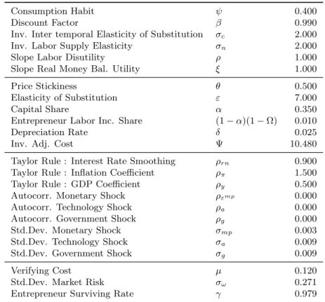
3.1 Model Parameters . . . 75
4.1 Lagrange Multiplier Tests for Linearity . . . 111
4.2 Parameters’ Range . . . 126
List of Figures
2.1 Transition Functions . . . 35
2.2 Comparison of the Second Order Logistic and Exponential Function . . . 40
2.3 Transition functions of STVAR :M odelB 1960Q2 to 1995Q2 . . . 41
2.4 Cumulative Responses of dy to dm : First Order Logistic STVAR . . . 42
2.5 Cumulative Responses of dp to dm : First Order Logistic STVAR . . . 43
2.6 Cumulative Responses of dy to dm : Second Order Logistic STVAR . . . 44
2.7 Cumulative Responses of dp to dm : First Order Logistic STVAR . . . 45
2.8 Cumulative Responses of dy to ff : Second Order Logistic STVAR . . . 46
2.9 Cumulative Responses of dp to ff : Second Order Logistic STVAR . . . 47
2.10 Cumulative Responses of dy to ff : Second Order Logistic STVAR . . . 48
2.11 Cumulative Responses of dp to ff : Second Order Logistic STVAR . . . 49
3.1 The Responses to Monetary Policy Shocks (mp),M odel1 . . . 88
3.2 The Responses to One Standard Deviation of Monetary Policy Shocks in Ex-pansions and Recessions : Demand Shocks, M odel1 . . . 89
3.3 The Responses to One Standard Deviation of Monetary Policy Shocks in Ex-pansions and Recessions: Supply Shock, M odel1 . . . 90
3.4 The Response to Monetary Policy Shocks (mp),M odel2 . . . 91
3.5 The Responses to One Standard Deviation of Monetary Policy Shocks in Ex-pansions and Recessions : Demand Shocks, M odel2 . . . 92
3.6 The Responses to One Standard Deviation of Monetary Policy Shocks in Ex-pansions and Recessions : Supply Shocks, M odel2 . . . 93
3.8 The Responses to One Standard Deviation of Monetary Policy Shock in
Expan-sions and RecesExpan-sions : Demand Shocks,M odel3 . . . 95
3.9 The Responses to One Standard Deviation of Monetary Policy Shock in
Expan-sions and RecesExpan-sions : Supply Shocks,M odel3 . . . 96
3.10 The Responses to Monetary Policy Shocks (mp),M odel4 . . . 97
3.11 The Responses to One Standard Deviation of Monetary Policy Shocks in
Ex-pansions and Recessions : Demand Shock (mp),M odel4 . . . 98
3.12 The Responses to One Standard Deviation of Monetary Policy Shocks in
Ex-pansions and Recessions : Supply Shock (mp),M odel4 . . . 99
3.13 The Responses to Monetary Policy Shocks (mp),M odel4 (Simple Taylor’s Rule) 100
3.14 The Responses to One Standard Deviation of Monetary Policy Shocks in
Ex-pansions and Recessions: Demand Shocks,M odel4 (Simple Taylor’s Rule) . . . 101
3.15 The Responses to One Standard Deviation of Monetary Policy Shocks in
Ex-pansions and Recessions: Supply Shocks, M odel4 (Simple Taylor’s Rule) . . . . 102
4.1 The Responses to Monetary Policy Shocks (mp). M odel1: Without Financial
Accelerator, Linear Phillips Curve. . . 142
4.2 The Responses to One Standard Deviation of Monetary Policy Shocks in
Ex-pansions and Recessions: Demand Shocks (government expenditure), M odel1:
Without Financial Accelerator, Linear Phillips Curve. . . 143
4.3 The Responses to One Standard Deviation of Monetary Policy Shocks in
Expan-sions and RecesExpan-sions: Supply Shocks (technology),M odel1: Without Financial
Accelerator, Linear Phillips Curve. . . 144
4.4 The Responses to Monetary Policy Shocks (mp). M odel2: With Financial
Accelerator, Linear Phillips Curve. . . 145
4.5 The Responses to One Standard Deviation of Monetary Policy Shocks in
Ex-pansions and Recessions: Demand Shocks (government expenditure), M odel2:
4.6 The Responses to One Standard Deviation of Monetary Policy Shocks in
Ex-pansions and Recessions: Supply Shocks (technology),M odel2: With Financial
Accelerator, Linear Phillips Curve. . . 147
4.7 The Responses to Monetary Policy Shocks (mp). M odel3: Without Financial
Accelerator, Nonlinear Phillips Curve. . . 148
4.8 The Responses to One Standard Deviation of Monetary Policy Shocks in
Ex-pansions and Recessions: Demand Shocks (government expenditure), M odel3:
Without Financial Accelerator, Nonlinear Phillips Curve. . . 149
4.9 The Responses to One Standard Deviation of Monetary Policy Shocks in
Expan-sions and RecesExpan-sions: Supply Shocks (technology),M odel3: Without Financial
Accelerator, Nonlinear Phillips Curve. . . 150
4.10 The Responses to Monetary Policy Shocks (mp). M odel4: With Financial
Accelerator, Nonlinear Phillips Curve. . . 151
4.11 The Responses to One Standard Deviation of Monetary Policy Shocks in
Ex-pansions and Recessions: Demand Shocks (government expenditure), M odel4:
With Financial Accelerator, Nonlinear Phillips Curve. . . 152
4.12 The Responses to One Standard Deviation of Monetary Policy Shocks in
Ex-pansions and Recessions: Supply Shocks (technology),M odel4: With Financial
Accelerator, Nonlinear Phillips Curve. . . 153
4.13 Unconditional Impulse Responses . . . 154
4.14 Impulse Responses to Moderate Contractionary Policies Implemented at
Reces-sions and ExpanReces-sions . . . 155
4.15 Asymmetric Effects of Contractionary Policies : Expansions over Recessions . . 156
4.16 Unexplained Asymmetric Effects of a Contractionary Policies: Expansions Over
Chapter 1
Introduction
Monetary policy was once believed to have symmetric effects on the economy. However,
there is evidence showing that the effects of the monetary policy on the economy might be
asymmetric. Friedman and Schwartz (1963) argue that the 1930 Great Depression could have
been just an ordinary recession if the Fed had not severely reduced money supply. However,
the stringent policies aiming at preventing the speculative attack drained out liquidity from
the economy and brought the economy to a deep recession. On the other hand, the efforts
of expansionary policies aiming at recovering the economy from a recession seem to be futile.
Milton Friedman compares the asymmetric effects of contractionary policies and expansionary
policies to a string –“Monetary policy was a string: You could pull on it to stop inflation but you could not push on it to halt recession. You could lead a horse to water but you could not make him drink.”
The asymmetry observed at business cycle peaks motivates a scientific investigation of
the effects of monetary policy in general. The work of Cover (1992) provides evidences of
the asymmetry. The author studies the effects of the monetary policy using money supply
as a policy instrument. The effects of contractionary policies were found to have stronger
effects on output than expansionary policies. Focusing on the money supply, other researchers
extend the scope of the study to other aspects of the asymmetry. Ravn and Sola (1997) find
shocks were found to have less effective on the output than small money supply shocks. Thoma
(1994) studies the role of the money supply over the business cycle and finds that monetary
policy has different effects on the output depending on the phases of the business cycle. The
author finds that tight monetary policies have stronger effects on the output during
high-growth periods, while easy policies have the same effects throughout the business cycle. Other
nonlinear econometric techniques are also used to find evidence of the asymmetry. Weise (1999)
applies a smooth transition vector auto regression (STVAR) to test the asymmetry and find no
evidence of the asymmetry between positive and negative money supply shocks. Instead, the
author finds that monetary policy has more impact on the output during recessions. Garcia
and Schaller (1995) use a Markov switching model to examine the effects of the policy using
the interest rate as the policy instrument. The policy was found to have stronger effects on
the output during recessions.
Altogether, there are at least three aspects of asymmetric effects of the monetary policy.
First, there are asymmetric effects between contractionary and expansionary policies. The
monetary policy is tested to see whether it has the same absolute effects to the economy.
Second, there are asymmetric effects between aggressive and moderate policies. The policy
is tested to see whether it has a proportionate scale in relation to the intensity of the policy.
Third, there are asymmetric effects of the policy through out the phases of business cycle. The
same policy is tested to see whether it has the same effects on the economy regardless of the
positions in the business cycle.
Several theoretical mechanisms have been proposed to justify the existence of asymmetric
responses to monetary policy shocks. Morgan (1993) has classified the theories into three
groups : a convex supply curve, a financial friction, and a change in economic outlook. A
convex supply curve explains the asymmetry through a mechanism of price stickiness (e.g.
Rotemberg (1982), Calvo (1983) and Ball and Mankiw (1994)). The tendency that the price is
sticky downward makes the supply curve a convex function. Thus, the effects of the monetary
policy depend on the portion of the supply curve in which the policy is implemented.
and borrowers. The lenders charge a risk premium to compensate the information risk and
the default risk (e.g. Bernanke et al. (1998)). The investment risk and borrowers’ net worth
position determine the risk premium. A risky project has a higher default risk. Thus, a higher
risk premium is charged. A higher borrowers’ net worth decreases a default risk. Therefore,
a lower risk premium is required. These factors determine the degree of financial accelerator
and thus determine the effects of the monetary policy.
The last group of theories deals with how people react to the phases of business cycle.
Dur-ing recessions, people might be insecure about the economic situations makDur-ing expansionary
policies ineffective. On the other end, people might be confident of the economic conditions
during expansions making contractionary policies ineffective. Should people be more
inse-cure in recessions than confident of expansions, monetary policy would be less effective on
the output during recessions than expansions. However, the explicit mechanism has not been
developed yet. It is more a discussion in the literatures than an established micro-founded
theory.
A question that has not been answered yet is how well those theories can account for the
asymmetry observed from data. Even though nonlinear econometric techniques have been
used to find the evidences of the asymmetric effects, those empirical works were linked to the
theoretical model via a reduced-form model. The direct application of an estimated model
that is supported by a reduced-form model suffers from Lucas’s critique in that the estimates
would experience a structural change through time due to the rational expectation hypothesis.
In addition, the contribution of a particular theoretical model in explaining the existence of
the asymmetry cannot be fully investigated via the reduced-form model. On the theoretical
side, an analysis in a nonlinear general equilibrium framework has not been undertaken due to
analytical difficulties and a high computational cost. Thus, most proposed explanations were
studied in a partial equilibrium framework (for example, Ball and Mankiw (1994)). Moreover,
when a model is analyzed in a general equilibrium framework, it is usually log-linearized before
further analyses are done (for example Bernanke et al. (1998)). Thus, the model lost its ability
How well can these theories explain the observed asymmetry? Do the existing theories
provide enough understanding about the mechanism by which the asymmetry is created? What
aspects of the theories have to be developed? To answer these questions, the performance of a
particular theoretical mechanism has to be investigated. A general equilibrium framework is
required to incorporate the interaction among sectors in the economy. The nonlinearity of the
model has to be preserved to establish a framework to investigate the asymmetry. Then, the
nonlinear general equilibrium framework could provide a channel to evaluate the performance
of the model in explaining the data.
This study investigates the ability of the existing theories to explain the observed
asym-metric effects of the monetary policy. Both empirical and theoretical models will be analyzed
in nonlinear systems to allow the possibility of the asymmetry. The following research
method-ology is proposed to evaluate a theoretical model.1
1. Estimate the effects of the monetary policy using a nonlinear econometrics technique
and measure the degree of the asymmetry.
2. Analyze the theoretical model in a DSGE model.
3. Find the solutions of the model by using a nonlinear solution method.
4. Produce a set of artificial data from the estimated DSGE model.
5. Apply the same technique in the first step to measure the asymmetry from the artificial
data.
6. Compare the degree of the asymmetry measured from the actual and the artificial data
produced by the model.
Completing the whole procedure will give an access to the ability of a particular model
in explaining the asymmetry. The results will provide some insights into the mechanism by
which the asymmetry is produced. This knowledge will be beneficial to set the direction of
1
the research about the asymmetry. This research methodology can also be applied to access
the performance of other alternative models along these lines.
The above procedure is implemented to investigate the asymmetric effects of the monetary
policy in the U.S. economy and accomplished in three chapters.
Chapter 2 completes the first step of the procedure. The chapter empirically investigates
the effects of the monetary policy. Among the choice of econometric techniques, smooth
transition vector auto regressive (STVAR) is employed. It describes the economy by a mixture
of two distinct VAR regimes. Each regime is weighted by a continued weighting function, a
transition function, whose value depends on the value of an observable variable, a switching
variable.
Chapter 3 completes the second and the third step of the procedure. It theoretically
in-vestigates two causes of asymmetric effects of the policy: convex supply curve and financial
friction. The financial friction is modeled by the Bernanke et al. (1998)’s financial accelerator
model and the convex supply curve is modeled by the nonlinear Phillips curve. The
conven-tional log-linearization or linearization cannot be used. A proper solution method will be used
to preserve the nonlinearity of the theoretical model. The solution of the model is obtained
by the second-order perturbation method. The model’s parameters are calibrated to the U.S.
economy. They are taken from Bernanke et al. (1998) and Gali and Rabanal (2004). Then
the asymmetric effects of the monetary policy are analyzed by using the impulse response
functions.
Chapter 4 accomplishes the procedure. This chapter estimates the model discussed in
chapter 3 by using indirect inference estimator, developed by Smith Jr (1993), Gourieroux et al.
(1993), Gallant and Tauchen (1996), and Keane and Smith (2003). The conventional maximum
likelihood procedure with the Kalman filtering is not applicable to this study. In order to use
the standard maximum likelihood procedure, the likelihood function of the model has to be
specified and the model has to be written in a space representation. However, a
linearization, or obtained by the first order perturbation method. Once the model is estimated,
it can be implemented to generate a set of artificial data, which is used calculate the implied
Chapter 2
Asymmetric Monetary Policy Responses in
the U.S. Economy : Smooth Transition
Vector Autoregressive
2.1
Introduction and Related Literature
Monetary authority can influence output and price level by adjusting the policy variable.
Responses to a policy change could vary depending on the circumstances. For example, Weise
(1999) finds that the responses of output are stronger during recessions. If monetary policy
has strong asymmetric effects, a standard VAR, which is a linear model, is not applicable. This
paper uses smooth transition VAR (STVAR) to study asymmetric effects of monetary policy
in the U.S. economy. Two forms of transition function in STVAR are considered: the
first-and the second- order logistic function. The asymmetric effects of monetary policy are studied
in three aspects: the effects of the policy during low versus high growth periods, the effects
of expansionary versus contractionary policies, and the effects of small versus large changes in
the policy.
Economic theories suggest possible asymmetric responses to monetary policy. The
supply side (see Karras (1996a)). For example, Caballero and Engel (1992) and Ball and
Mankiw (1994) develop models in a sticky price context, which leads to a convex aggregate
supply curve. The convex aggregate supply curve predicts that output will be more sensitive
to the policy during recessions than booms, and more sensitive to big than small changes in
the policy. For aggregate demand side, Bernanke and Gertler (1989), Bernanke et al. (1998)
Bernanke and Blinder (1992) develop a financial accelerator model in which the firms’ balance
sheet conditions can amplify the effects of the policy on output. Firms borrow funds from
fi-nancial institutions with a risk premium rate, which depends on firms’ balance sheet position.
This so-called external risk premium is higher when firms have credit constraints, for example
when contractionary policy is implemented or during recessions, or both.
Recent studies in asymmetric effects of monetary policy are sparked by Cover (1992). Using
U.S. data, Cover finds that output responds differently to positive and negative supply shocks.
This evidence is supported by DeLong et al. (1988), Morgan (1993), Rhee and Rich (1995),
Thoma (1994), Kandil (1995) and Karras (1996a). Thoma (1994) finds that only negative
money supply shocks have strong effects in recessions but not in booms, while positive shocks
have no asymmetric effects. However, Ravn and Sola (1997) argue that the asymmetry found
in Cover (1992) arises from changing in the policy regime. After controlling for the policy
regime change, the asymmetry between positive and negative supply shocks disappears. On
the other hand, Ravn and Sola (1997) find evidences supporting menu cost model where
large and small shocks have different effects. The above studies test the asymmetry using
a threshold VAR-type model. Weise (1999) applies a smooth transition VAR to test the
asymmetric responses to monetary policy and finds no evidence of asymmetric effects of positive
and negative shocks. Conversely, Weise confirms that monetary policy has greater impacts on
output during recessions. Garcia and Schaller (1995) use a Markov switching model to examine
the effects of the policy during expansions and a recessions and find stronger effects of the policy
during recessions. In summary, there are empirical evidences supporting the asymmetric effects
of monetary policy. The policy has stronger effects during recessions. However, the results are
VAR1 assumes that the relation among the variables in the system is linear and stable over
time. The above findings reject the traditional VAR in favor of a nonlinear model. Alternative
methods to study a nonlinear system have been developed and can be broadly classified into
three categories: Markov switching model, threshold VAR model and smooth transition VAR
(STVAR) model.
Hamilton (1989) and Diebold and Rudebusch (1989) develop Markov switching model to
study business cycle. The model describes the economy under two regimes: for instance,
expansions and recessions. The economy is allowed to switch from one to another regime.
These regimes are unobservable and migrating according to a stationary migrating
probabil-ity. This model is very useful when the number of regime is as small as two, but becomes
computationally complicated as the number of regime increases. However, Boldin (1996) and
Potter (1995) suggest that there should be at least three regimes to describe the economy.
In addition, the Markov switching model assumes that the regime switches are driven by an
unobservable variable, which does not provide the intuition behind the asymmetric effects of
monetary policy.
Tsay (1989) develops threshold VAR model as an alternative to Markov switching model.
Similar to Markov switching model, the model describes the economy under multiple regimes.
At any point of time, one regime is selected with probability one. The regime is identified
by an observable variable called switching variable. When the switching variable falls into a
particular range of value, a corresponding regime is selected. The threshold VAR is particularly
useful when there are more than two or three regimes. In the same way as Markov switching
model, threshold VAR also discretely switches from one to another regime. However, it is very
unlikely that the economy will jump between the regimes.
Granger and Ter¨asvirta (1993), Ter¨asvirta (1996) and Dijk et al. (2002) develop a smooth
transition VAR (STVAR) to allow the regression coefficients to change smoothly from one
regime to another. In addition, the transition is endogenously determined by an observable
1
switching variable which provides economic intuition for the regime changes. An attribute
of STVAR is that the deviations from equilibrium creates mean reversion behavior whose
character depends on the transition function. The linear logistic function implies asymmetric
behavior depending on whether the switching variable is above or below the equilibrium, for
example the business cycle (Weise (1999), Bec (2000), Rothman et al. (2001), Lundbergh
et al. (2003), Petersen (2007)). The quadratic one indicates different pattern between medium
and extreme regimes, for example an exchange rate zone and an inflation targeting where
authorities response more aggressively to a larger deviation from the target (Taylor et al.
(2001), Martin and Milas (2004), and Sollis (2008)).
The aim of the monetary policy is to stabilize economy, which establishes nonlinear
rela-tionships and mean revision behaviors. Therefore, this paper uses STVAR model to capture
the nonlinear effects of monetary policy. The rest of this paper is organized as follows. First,
the economic theory predicting asymmetric response to the policy is discussed. The procedures
to test nonlinearities and to set up a STVAR model are explained in the methodology section.
Finally, the empirical results for the U.S. economy are presented.
2.2
Theoretical Framework
This section lays down a simple aggregate macro-model that allows for the asymmetric effects
of monetary policy. The model in this section closely follows Weise (1999) and is augmented by
a financial accelerator. The model starts with a simple log-linearized macro model of aggregate
demand, aggregate supply and policy rule. The sources of nonlinearity are the friction in the
price level and the friction in financial markets.
The simple aggregate supply is derived from a short run production function with fixed
nominal wages Yts = f(θt, K, W /Pt). Because of the fixed level of capital ¯K and nominal
lagged endogenous variable Xt−1 and the supply shock θt,
yts=b0+b1pt+S(L)Xt−1+θt, (2.1)
where S(L) is a lagged polynomial and yt is equilibrium output growth. The endogenous
variableXt depends on the choice of the policy variable, which will be discussed shortly. The
output growth yts deviates from the constant levelb0 by the inflation pt and the productivity
shockθt.
The aggregate demand is a function of market interest rate,rmt , inflation rate,pt, a lagged
endogenous variable,Xt−1, and a demand shock, νt,
ytd=a0−a1rmt −a2pt+A(L)Xt−1+νt. (2.2)
Monetary policy is assumed to follow Taylor’s rule, given in Equation 2.3.
rt=r0+r1yt+r2pt+R(L)Xt−1+εrt. (2.3)
However, the authority can choose money supply as the policy instrument as well. Money
supply growth mt and the nominal interest rate rt are reciprocal in this model. Equation 2.4
describes the relationship between the money growth and the interest rate. For illustration
purpose, the equilibrium condition is derived by using the growth rate of money supply as the
policy variable. Thus, the endogenous variables are Xt = [yt, pt, mt]0. The monetary policy
equation is rewritten as in Equation 2.6.
mt = M0−λrt. (2.4)
mt = (M0−λr0)−λr1yt−λr2pt−λεrt. (2.5)
mt = m0−m1yt−m2pt+M(L)Xt−1+εmt , (2.6)
The equilibrium interest rate rmt need not equal the risk free ratert. This will be the case
only when the financial friction is not functioning. Bernanke et al. (1998) show that the
asym-metric information between the borrowers and the lenders creates an external risk premium.
The premium will be increased when the borrowers have weak balance sheet positions. The
premium is also higher during recessions because of a higher default risk.2 Thus, the policy
will affect the economy through both liquidity and credit channels.3 The credit channel,
how-ever, influences the economy only in an intermediate range. Under severe economic conditions,
where the credit constraint strictly binds, the lenders require a very high-risk premium. All
firms will face the credit constraint. The credit channel will not function, reducing the effect
of the credit channel mechanism. The relationship between the equilibrium rate and the risk
free rate can be summarized as follows,
rmt =b(zt, Wt)rt, (2.7)
wherezt is a variable indicating the level of information asymmetry. The risk premium equals
zero when there is no asymmetric information b(·) = 1 and is a decreasing function of net
worth,∂b(·)/∂Wt<0. The aggregate demand in Equation 2.2 can be rewritten as,
ytd=a0−a10(zt, Wt)rt−a2pt+A(L)Xt−1+νt. (2.8)
wherea01(zt, Wt) =a1b(zt, Wt). The degree to which the asymmetric information and the net
worth affect the risk premium depends on many factors, including the phase of business cycle,
the degree of credit constraint faced by the firms and the investigating cost when the loans are
default.
The last key variable in this system is the inflation rate pt. The free market equilibrium is
2This derivation can be found in Bernanke et al. (1998). 3
the level of p0t that clears aggregate demand and aggregate supply in Equation 2.8 and Equa-tion 2.1, respectively. The interest rate in EquaEqua-tion 2.8 is eliminated by using EquaEqua-tion 2.4.
The aggregate demand can be rewritten as in Equation 2.9 and the free market equilibrium
inflation rate is given in Equation 2.10,
ydt =
a0−
a01(·)M0
λ
+a
0
1(·)
λ mt−a2pt+A(L)Xt−1+νt, (2.9)
Pt0 = 1
b1+a2
a0−b0−
a01(·)M0
λ
+a
0
1(·)
λ mt+A(L)Xt−1+ (νt−θt)
. (2.10)
Another friction in the model is nominal price rigidity. The price adjustment in this model
follows Calvo’s price setting where only a fraction, 1−α(xt), of firms can adjust the prices
at each time. The firms who can change their prices set the prices at the market equilibrium
price and the other hold their last period prices. Equation 2.11 represents the Calvo dynamics
of price, where Pt is log of aggregate price level andPt∗ is log of optimal price.
Pt=α(xt)Pt−1+ (1−α(xt))Pt∗ (2.11)
The firm choosesPt∗ to maximize expected discounted profits subject to the discount factor
β and the sticky price parameterα(xt). The optimial price can be expressed as:
Pt∗ = (1−βα(·)) ∞ X
i=0
(βα(·))iEt
Pt0+i. (2.12)
Let pt = Pt−Pt−1 denote the inflation rate at t, use Equation 2.11 and Equation 2.12 to
obtain
pt=κ(·)Pt0+βEtpt+1, (2.13)
to obtain
pt−1 =
(1−α(·))2
α(·) P
0
t−1+Et−1[pt],
(1−L)pt =
(1−α(·))2L
α(·) P
0
t +g(t),
pt =
(1−α(·))2
α(·)
L
(1−L)
Pt0+ g(t) (1−L).
Finally, substitute definition of Pt0 from Equation 2.10 to obtain the inflation dynamic
pt =
(1−α(·))2
α(·)
L
(1−L)
1 b1+a2
a0−b0−
a01(·)M0
λ
+a
0
1(·)
λ mt+A(L)Xt−1+ (νt−θt)
+ g(t)
(1−L). (2.14)
As in a standard Calvo price model, the equilibrium pricept will collapse to the free market
equilibrium price where all firms can adjust the prices, αt = 0. The extension from the
standard Calvo here is that the stickiness parameterαt(xt) is allowed to change depending on
a switching variablext. Note that the price friction might come from other sources. However,
those sources of stickiness can be captured by state dependent stickiness parameter αt(xt).
Thus, the candidate for the switching variable can be any key economic variables, e.g. inflation
rate, output growth and money supply growth. Using a menu cost model, Ball and Mankiw
(1994) predict asymmetric responses to a policy in the different economic situation. During
periods of high economic volatility or inflation, firms can change their prices at a relatively low
cost, resulting in a small degree of stickiness. The policy will be less effective on output. On
the other hand, when the economy is stable, firms face a higher menu cost yielding a higher
degree of stickiness and intensifying the effect of the policy on output.
To reduce the number of variables in the system, the variables zt, Wt and xt, which
de-termine the policy effectiveness a0(zt, Wt) and price stickiness α(xt), are linked to a
com-mon switching variable st through functions z(st) : st → zt, W(st) : st → Wt and x(st) :
To transform this structural model into an econometric model, the equilibrium equations
in Equation 2.9, Equation 2.14, and Equation 3.33 are written in a matrix form:
Xt=X0+B1Xt+B(L)Xt−1+C(L)t, (2.15)
where,
X0 =
b0
(1−α˜(st))2
˜
α(st)
L
(1−L)
1
b1+a2
a0−b0−˜a1(sλt)M0
m0 ,
B1 =
0 b1 0
0 0 (1−α˜(st))2
˜
α(st)
L
(1−L)
1
b1+a2 ˜
a1(st)
λ
−m1 −m2 0
.
t= [θt, νt, εmt ]0 is the vector of structural shocks and B(L) andC(L) are lag-polynomials of
endogenous variables and structural shocks, respectively. These structural equations can be
transformed to an estimable reduced form by grouping Xt, then multiplying both sides by
(I −B(L))−1, assuming that (I −B(L)) in invertible. The reduced-form VAR is then given
by,
Xt=D0+D(L)Xt−1+ut, (2.16)
where D0 = (I−B0)−1X0,D(L) = (I−B0)−1B(L), andut= (I−B(L))−1C(L)t. If the
stability condition holds, this reduced-form VAR is estimable.
The structural parameters can be recovered by putting identification restrictions. The
traditional Cholesky decomposition for a short-run identification scheme is applied. The output
is assumed to have no contemporaneous movement to price and monetary policy. Price level
can be influenced by output, but not by the policy. Lastly, the monetary authority makes the
2.3
Methodology
This section covers the main tools to test the asymmetric effects of monetary policy. Since
STVAR is an extension of standard VAR, the procedures start from setting a standard VAR.
The degree of nonlinearity is then tested. If there is evidence of nonlinearity, a transition
function for STVAR is chosen. Once the STVAR is formulated, a general impulse response
function is applied to study the dynamic effect of the policy.
2.3.1 STVAR
STVAR constructs infinite VAR regimes from two distinct VAR systems. The terminology
“smooth transition” emphasizes how this model changes the regimes. The two VAR systems
are weighted by a smooth weighting functionf(st) whose value depends on a switching variable
st. Though there are only two distinct regimes, the resultant regime can be infinite. This
feature is different from Markov switching model, which assumes that the transition between
the regimes is binary. Thus, the terminology “regime” in STVAR context is not necessarily a
low and high growth regime. The structure of STVAR is described in Equation 2.17a.
Yt = (1−f(st)) (A0+A(L)Yt−1) +f(st) (C0+C(L)Yt−1) +ut (2.17a)
Yt = A0+A(L)Yt−1+f(st)(C0−A0
| {z }
B0
+ (C(L)−A(L))
| {z }
B(L)
Yt−1) +ut (2.17b)
Yt = A0+A(L)Yt−1+f(st)(B0+B(L)Yt−1) +ut (2.17c)
When function f(st) equals zero, the system follows the regime A, Yt = (A0+A(L)Yt−1)
and follows the regime B, Yt = (B0+B(L)Yt−1) if f(st) equals one. Equation 2.17a and
Equation 2.17c are equivalent. However, Equation 2.17c is more convenient for estimation
purposes. Equation 2.17c takes regime A as an anchor regime and takes regime B as an
increment to the anchor regime.
s(t). However, the logistic and exponential functions are particularly useful in the business
cycle context because of their simplicity and parsimony.4 The first-order and second-order
logistic transition and exponential transition functions are represented by Equation 4.2,
Equa-tion 4.3 and EquaEqua-tion 2.20, respectively.
f(st) =
1 +exp
−
γ(st−c) σst
−1
;γ >0 (2.18)
f(st) =
1 +exp
−
γ(zt−c1)(st−c2)
σst
−1
;γ >0, c1 ≤c2 (2.19)
f(st) =
1−exp
−γ(st−c)2 σst
;γ >0 (2.20)
In each function, the shape of the function is governed by slope γ and location c. The
locater of the second-order logistic function is {c1, c2}. The transition function is scaled by
the sample standard deviation of the switching variable, σst.
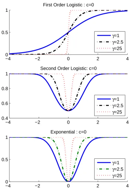
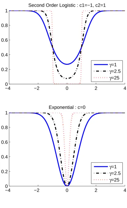
Figure 2.1 and Figure 2.2 compare logistic and exponential transition functions. Each
function is evaluated at c=0 and γ = 1, 2.5 and 25. When the slope converges to zero, the
function becomes linear. On the other hand, the function converges to a step function and the
system becomes a threshold VAR when the slope approaches infinity. The logistic function
approaches one when the value of the switching variable is greater than c and conversely
approaches zero. The exponential function equals one when the switching variable deviates
from the center. The second-order logistic and exponential functions have a similar form except
that the logistic function has a minimum weight at 0.5. This difference will result in a different
scale of the estimates in Equation 2.17c but the resultant impulse response functions are the
same. The second-order logistic function has another interesting feature when c is split into
c1 and c2 and when the value of the slope is high. The resultant transition function allows
the zero weight area to be in a range [c1, c2], instead of a single value c. In addition to the
first-order logistic function, this paper applies the second-order logistic function to allow a
possible intermediate range.
The first-order and the second-order logistic functions are useful in different circumstances.
The first-order logistic function is more appropriate if the regime changes monotonically to
the level of the switching variable. For example, modeling expansion and recession regimes
can be done by using the output growth as a switching variable with the first-order logistic
function. With a zero location parameter, the logistic function places a weight of one when
the output growth is greater than zero, and a weight of zero when output growth is negative.
Referring to Equation 2.17a, the recessions are described by regime A and expansions are
described by regime C. Alternatively, the second-order logistic function is suitable for modeling
intermediate and extreme regimes: for example, the credit constraint model. In the normal
economic condition, the credit channel amplifies the monetary policy making the policy more
effective. When the credit constraint binds excessively, the role of the financial accelerator is
mitigated, resulting in less policy effectiveness. In this situation, the regime of STVAR is not
a high and low growth regime but an intermediate-extreme regime. In addition, the policy
variable itself can be a switching variable. Following Taylor’s rule, a larger change in policy is
expected when the output and inflation deviate too much from the target values.
2.3.2 Nonlinearity Test
A nonlinearity model would be redundant and less efficient if the true model is in fact a linear
model. This section discusses how to test nonlinearity in a VAR system. If the nonlinearity is
detected, the model is further investigated to choose a transition function.
Testing linearity in STVAR is equivalent to testing that parameters in two regimes are
identical, assuming that the true switching variable is known. Under this null hypothesis,
the standard Wald test for nonlinearity is not applicable. The linearity assumption implies
that B0 and B(L) in Equation 2.17c equal to zero. In this situation, the changes in slope
and location parameters do not affect the likelihood value. Ter¨asvirta and Anderson (1992)
suggest the linearity hypothesis is also equivalent to the hypothesis that γ = 0. Thus, the
system can be approximated by the first-order Taylor’s expansion around the neighborhood of
a three-step procedure test for nonlinearity. This procedure is also applied in Weise (1999) to
test the nonlinearity in a VAR system for studying the asymmetric effects of monetary policy.
The three steps are:
1. Run the standard regression to get the residualuˆt
Xt=D0+
p
X
i=1
D1iXt−i+ut
2. Run the auxiliary regression to get the residualvˆt
ˆ
ut= Γ0+
p
X
i=1
Γ1iXt−i+ p
X
i=1
Γ2istι0(n)Xt−1+vt (2.21)
3. Compute the likelihood ratio test LR=T(log|Ω0| −log|Ω1|)
The unit vector ι in the second step is introduced to allow the column-wise
multiplica-tion between the endogenous variable Xt−1 and the switching variable st. T is the number
observations and p is the number of VAR lag. Ω0 = ˆu0ˆu/T and Ω1 = ˆv0ˆv/T are the
es-timated variance-covariance of the restricted and the unrestricted model, respectively. The
statistic is the nonlinearity test for the whole system. The asymptotic distribution of the test
is χ2(pk2). Thejthindividual equation can be tested by replacing the variance covariance by
the jth diagonal element of the variance-covariance matrix. The degree of freedom is now
reduced to pk. Ter¨asvirta and Anderson (1992) also suggest using the F version of the LM
test for a small sample to correct for the small sample bias. The F statistic is computed by
[(ˆu0iuˆi−ˆv0iˆvi)/pk]/[uˆ0iˆui/(T−2pk−1)].
Luukkonen et al. (1988) argue that this procedure has a low power test when the switching
variable is one of the endogenous variables or the transition function is one of the endogenous
an augmented version of Equation 2.21:
ˆ
ut = Γ0+
p
X
i=1
Γ1iXt−i+ p
X
i=1
Γ2istι0(n)Xt−1+vt
+
p
X
i=1
Γ3is2tι
0
(n)Xt−1+
p
X
i=1
Γ4is3tι
0
(n)Xt−1 (2.22)
The linearity hypothesis is Γ2 = Γ3 = Γ4 = 0. This paper finds that the Luukkonen et al.
(1988) adjustment obtains too strong power of the test so that the null hypothesis is always
rejected at any level of significance. Due to its strength, the test is uninformative for the choice
of an appropriate switching variable. Tsay (1989) and Ter¨asvirta (1994), on the other hand,
suggest choosing the variable that gives the lowest p-value of the test. Using a wrong switching
variable, the p-value of the test will increase due to the misspecification error. Moreover, the
rank of the variable by p-value from these tests is very similar. Hence, this paper applies the
test proposed by Ter¨asvirta and Anderson (1992).
2.3.3 Choosing the Transition Function
Luukkonen et al. (1988) and Ter¨asvirta and Anderson (1992) suggest further that the auxiliary
regression in Equation 2.22 can also be used to choose between the first-order and the
second-order logistic function (or exponential function). The method is based on a sequence of nested
hypotheses.
1. H01: Γ2= 0|Γ3= Γ4= 0,
2. H02: Γ3= 0|Γ4= 0,
3. H03: Γ4= 0,
The first hypothesis is essentially the linearity test. The test statistic is a traditional LR
statistic, which has the asymptoticχ2(pk2) distribution. Conditional on rejecting the linearity hypothesis, the logistic function should be chosen ifH03 is rejected. IfH03is not rejected but
rejected, the function with the lowest p-value should be chosen. This nested test is based on
the misspecification error test discussed above. In addition, an exponential or a second-order
logistic function has a quadratic form, while the first-order logistic function has a linear or
cube function. The H02 hypothesis tests the significance of the squared term of the switching
variable. Therefore, it validates a second-order logistic function.
Recall that all the tests above assume that the switching variablestis known. The switching
variable can be any variable and the switching function can take any functional form. This
study focuses only on variables suggested by the theory, (i.e. output growth, price level, and
monetary policy). In addition, the first difference of these variables is included in the possible
set of switching variables. These variables are the endogenous variables in the system. The
delay of each variable is also included to allow for possible lag responses.
2.3.4 Generalized Impulse Response Function
The impulse response function represents the response of the system to shocks over time. In a
linear system, the impulse response is invariant to characteristics and history of shocks. In a
nonlinear system, the system responds not only to the shocks, but also to the propagation of
the shocks. The impulse responses in a nonlinear system cannot be obtained analytically but
only by simulation. Koop et al. (1996) develop a “generalized impulse response function” to
study the responses in a nonlinear system. Their procedure is summarized as follows:
1. Set the initial state by picking a part of actual data denoted as Ωk t−1.
2. Design a hypothesized shock, e.g. the policy shock, denoted as∗0.
3. Randomly draw a q-period shock with replacement from the estimated residual, denoted
by jt, which have qk5 dimension, where q is the time horizon of the impulse response function and k is the number of endogenous variables. To allow the correlation among
the shocks, all k-shocks in the same period are picked.
4. Construct a benchmark path by feeding the model with a zero shock at periodt= 0 and
qt later on, denoted byGI0ki(Ωk t−1,0,
j t).
5. Construct a hypothesized path by feeding the model with a hypothesized shock, j0, at period t= 0 and qt later on, denoted byGI1k(Ωki
t−1, ∗0,
j t).
6. Repeat steps 2-4 B times.
7. Repeat steps 1-5 R times.
8. Compute an average impulse response functionGIbyPR
k
PB
j (GI1k((Ωkit−1, ∗0,
j
t)−GI0ki(Ωkt−1,0,
j
t))/BR,
or a median impulse response function by median
((Ωki t−1, ∗0,
j
t)−GI0ki(Ωkt−1,0,
j t))
The initial states in the first step are classified into two sets: low growth and high growth,
distinguished by standard deviation of output growth. High growth period is defined by that
the output grows at a faster rate than one standard deviation. What is left is classified as
the low growth period. Alternatively, the medium growth period can be introduced by using
the value of growth between the zero and the one positive standard deviation. However, the
results in this period are very similar to the low growth period as a whole. Thus, the medium
growth period is combined to the ones in the low growth period in the first definition.
The random draw in the third step and the repetition in the seventh step are done in
the period classification. For example, when considering a high growth period, all shocks are
drawn from the period where output growth is greater than one positive standard deviation.
Similarly, all initial states are in the high growth period. All possible initial periods are used
in repetition in the seventh step. The number of bootstrap repetitions in the sixth step is set
at 100.
2.3.5 Estimation
In principle, a STVAR structure in Equation 2.17c can be estimated by maximum likelihood
estimation will take a long time to obtain the global maximum value. On the contrary, given
particular values of the slope and location parameter(s), the system is reduced to a simple
linear VAR system. Assuming that there is no serial correlation in the residual matrix, the
OLS method yields the same estimates as a maximum likelihood estimator.
This paper adopts a grid search method to obtain the estimates. The procedure is:
1. Given a switching variable st, pick a value of slope and locators, denoted as, γ0 andc0.
2. Construct a weighting seriesf(s(t), γ0, c0) and generate a column wise multiplication of endogenous variables andf(s(t), γ0, c0), as in the second part of Equation 2.17c.
3. Estimate Equation 2.17c using OLS, collect the residual ˆu and calculate Ω = ˆu0uˆ0/T.
4. Use an optimization technique to minimizelog|Ω|.
This paper uses a grid search to find the optimal value of γ and c. The value of γ ranges
from 0 to 100 with the step size equals to 0.1. The location parameter is searched over the
actual value of the variable using as a switching variable. Weise (1999) also applies a similar
procedure except that he fixes the location parameter to zero for output growth and inflation
rate and at the mean for other variables. This assumption for both output growth and inflation
rate is valid but too restrictive. It is possible that the regimes could be separated somewhere
above or below zero. This paper allows the location parameter to change in a certain range.
To obtain a good scale parameter, there must be enough observations in the tail area of
the weighting function. For this purpose, the set of possible values is between at 20 and 80
percentile.
2.4
Empirical Results
Following Bernanke and Blinder (1992), this paper takes the federal funds rate as a policy
the different policy choices in the subsample covering 1960Q2 to 1996Q4. Weise (1999) uses
money supply as the money policy instrument to study the asymmetric effects of the policy
covering this subsample. Thus, Weise (1999)’s results are reproduced to compare with ones
of the interest rate model. Hereafter, the model using the federal funds rate and the money
supply as a policy variable will be referred to as M odelAand M odelB, respectively.
The data in this study are quarterly data of the U.S. economy. The set of endogenous
variables in each model are different. M odelA uses real GDP for output, GDP deflation for
price and the federal funds rate for the policy variable. The commodity price is also added
to the model to solve the price puzzle. M odelB uses the industrial production (IP) index for
output, the CPI for price level, and M1 as the policy variable.6 All the data in this paper are
obtained from the International Financial Statistic (IFS), except commodity price, which is
obtained from the Global Financial Data (GFD).
All data, except IP and M1 in the subsample, exhibit a unit root and need to be adjusted.
To obtain stationary series, all data are transformed by log differencing, except the federal
funds rate that needs only the first difference transformation. The inflation rate is multiplied
by four to get an annualized rate. Moreover, the data are filtered to remove seasonal movement
and possible structural breaks. Ravn and Sola (1997) show that the asymmetric effects found in
Cover (1992) disappear when the structural breaks are removed. The same filtering technique
is also applied in Weise (1999). Three possible structural break points are considered. The
first break is the oil shock of October 1973. The second break is the shifting in policy regime of
the Volcker period when the Fed abandoned the interest rate targeting and adopted a money
supply targeting. The third break is the evidence of the sharp decline in output volatility in
1985.7 The timing of the third break is about the same as of the starting period of Greenspan.
To avoid too much filtering, only 1985 is selected. The data are regressed on constant, seasonal
dummies, dummies for post- 72, post- 79 and post- 84 periods, a time trend and the time trend
6Generally, real GDP is applied to proxy output level in quarterly data. Industrial production index is used
in this case to obtain a result comparable to Weise (1999).
interacted with structure break dummies. In his study, Weise (1999) does not use the post 84
periods dummy to filter the data. Thus, to obtain a comparable result, filtering process in the
first subsample omits the post 84 periods dummy.
In both sample periods, the number of lags in the VAR is set to four. Setting the
max-imum lag at eight, three statistical criteria suggest the optimal lag at two or three. Those
tests are the lag exclusion test, Akaike’s information criterion (AIC) and Schwarz Information
Criterion (SIC). Increasing the number of lags in the VAR reduces the degrees of freedom but
increases the explanatory power of the data. Since the data are quarterly, a four-lag VAR can
better capture the cyclical movement during the year. Using the four-lag structure also avoids
unnecessary nonlinearity.
2.4.1 1960Q2 to 1995:Q2
Comparing Between the First- and the Second-Order Logistic STVAR
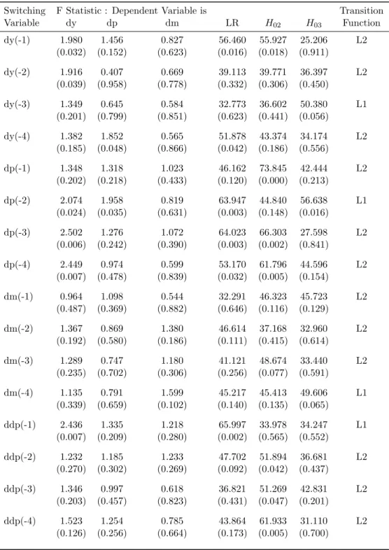
Table 2.1 reports a linearity test of M odelB. The linearity test for individual equations is
reported in column 2 to 4 and the whole system test is reported in column 5. The next two
columns report the hypothesis test ofH02 and H03, respectively. The last column indicates a
preferred transition function. The letter “L1” denotes the first-order logistic function and the
letter “L2” refers to the second-order logistic function.
The first four possible candidates for a switching variable are the first lag of change in
inflation rate, ddp(−1), the second and the third lag of inflation,dp(−2) and dp(−3), and the
first lag of output growth, dy(−1). The linearity assumption is rejected in all four cases. As
noted in Weise (1999), there is no evidence suggesting that money supply growth is a possible
switching variable. However, this does not necessarily mean that there is no asymmetric effects
of monetary policy. It only implies that money supply growth cannot indicate the transition
between the regimes. A striking result is that the second-order logistic function is a preferred
transition function in 12 out of 16 cases. This suggests that assuming only first-order logistic
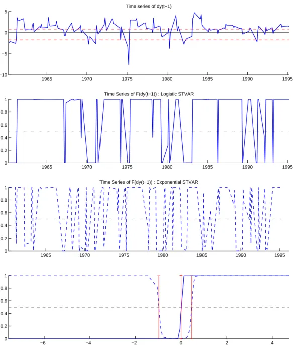
The different implications of the first- and the second-order logistic are investigated in
Figure 2.3. The first lag of the output growth is selected to be a case study since it is the
only one case reported in Weise (1999). The slope in the first-order logistic STVAR is 67.75
and the locater is restricted to 0. While these parameters are 14.15 and (-0.97,0.47) in the
second-order logistic STVAR. The top panel is a time series plot of the first lag of output
growth. The parallel dash lines are the second-order logistic locator. The time series of the
logistic function is plotted in the second panel. When the value of the lag output growth
is greater than zero, the transition function is one, and moves to zero when the lag output
growth is lower than zero. The third panel displays the time series of the second-order logistic
transition function. The function gives the value one when the lag output growth deviates
from zero too much on either side. When the deviation is small, however, the function gives a
weight of zero. The criterion for big and small is justified by two locater variables. The last
panel plots the shape of both functions for comparison. Both functions have high slope values
so they migrate from one to another regime quite rapidly around the locater variables. The
two functions are similar when the lag output growth is greater than zero. However, while
the second-order logistic function returns to one when the lag output growth is negative, the
first-order logistic function moves to another regime. The simulated impulse responses are
called for examining the different results.
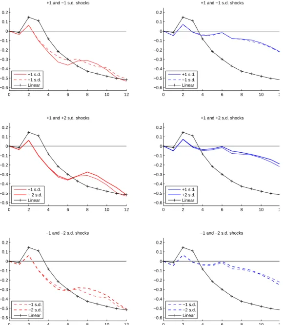
Figure 2.4 and Figure 2.5 are cumulative generalized impulse responses of output and price
to money supply shocks, respectively. These are the impulse response functions of M odelB
associated with the first-order logistic STVAR. Figure 2.6 and Figure 2.7 serve the same
purpose of the study for the second-order logistic STVAR.
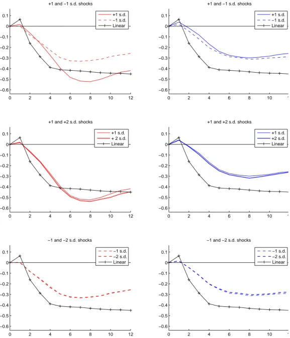
To compare the results with Weise (1999)’s, cumulative responses are used to examine the
net effects of the policy on the variables. The responses can be interpreted as total responses
to a permanent change in money supply. The responses in low and high growth periods are
displayed in the left and right panel, respectively. On the right panel, the initial periods are
high growth. The size of the shocks is one and two standard deviation. The top panel compares
down to be compared to responses to positive shocks. The second panel compares responses
to positive shocks of size 1- and 2- standard deviation in a similar way as those of negative
shocks are flipped up or down. The last panel compares responses to negative shocks of size
1- and 2- standard deviation. In every case, the impulse responses from the baseline VAR are
plotted to be benchmark functions. The comparison between the responses to small and large
shocks needs more clarification. The different size of the shocks definitely affects the economy
in the different scales. Whether the effects are proportionate to the size of the shocks is the
central question. The responses to 2-standard deviation shocks are scaled down by the factor
of two. If the policy does not have asymmetric effects between the different size of the shocks,
the impulse responses should lie on top of each other.
The impulse responses of the output to the policy shocks have the traditional hump-shaped
curves. The output increases in the first two quarters and starts to decrease. The output level
is still positive until the fourth quarter. The size of the shocks is one standard deviation, 1.56
percent. A one positive standard deviation shock results in a 0.5 percent decreases in output
at 3 years later. The policy shock increases the price level throughout the horizon. The price
level increases about 1.2 percent and stays at that level after 3 years elapsed.
For the first-order STVAR, hereafter L1-STVAR, there is the evidence supporting
asym-metric responses of output to the policy in low growth period. The output increases for two
quarters and decreases until the sixth quarter. The effect reverses for a short time at the
seventh quarter and then continues decreasing again at the eight quarter. Conversely, the
output responses are less sensitive when the policy shocks occur in a high growth period.
The total effect on the output is about 0.2 percent after 12 quarters. The output responds
symmetrically to small and large shocks. The responses to a one and two standard deviation
shocks virtually lie on top of each other regardless of the shocks. The only asymmetric effect
of the policy is the responses to the different direction shocks in the low growth period. The
conclusion for the asymmetric responses of the price level is similar to that of the output. The
only possible asymmetry is the responses to shocks during low and high growth period. The
output responses. Comparing to the baseline VAR, all price responses in STVAR model are
less sensitive.
The second-order logistic STVAR, hereafter L2-STVAR, gives the same conclusion about
asymmetric responses but it produces meaningful impulse responses for output. First, the
output is also more sensitive to shocks during low growth period. However, in this case,
the standard VAR model is roughly an average of both periods. L2-STVAR also predicts no
asymmetric responses to the different size of the shocks. Asymmetric responses to positive
and negative shocks become more obvious in this case. The two different responses have an
average around the baseline VAR. The responses of the price level are also similar but become
more sensitive. Quantitatively, the total effects of the shocks are about a half of the baseline.
Price level is less sensitive to shocks during high growth period. In addition, the asymmetric
effects between difference size of the policy shocks on output are not found. Similarly, the
asymmetric responses to positive and negative shocks are clearer than those of L1-STVAR.
The asymmetric responses of price level and of output are related to each other. Monetary
policy has no effect on output if price is perfectly flexible. The policy will affect the output
only if there is price friction. The less sensitive the price response, the more effective the policy
is. Thus, if there is no asymmetric of the price responses, the output is expected to have no
asymmetry as well.
In summary, both L1- and L2- STVAR show asymmetric effects of monetary policy in low
versus high growth periods. The output is more sensitive to the policy when the economy is in
low growth period. The price is less sensitive to the shock in high growth period. Asymmetric
effects of the size of shocks are not found. There are some evidences for asymmetric responses to
positive and negative shocks. However, L2-STVAR produces results that are more prominent.
STVAR: M odelA
This section discusses the results obtained fromM odelA, which uses the federal funds rate as
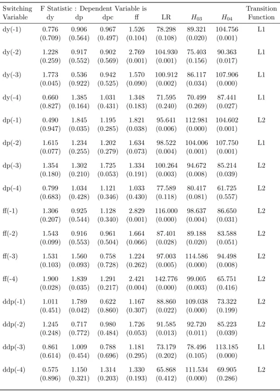
The first four possible candidates for a switching variable are the forth and the first lag
the federal funds rate, f f(−4), and f f(−1), the second and the third lag of output growth,
dy(−2) anddy(−3). Similar to the previous section, the linearity assumption is rejected in all
four cases. The second-order logistic function is preferred to be a transition function in 10 out
of 16 cases. There are two interesting points between these two models. First, when the federal
funds rate is used, the policy variable turns to be an important switching variable. Second,
the L2-STVAR is prominent if the switching variable is the federal funds rate. This suggests
that STVAR regime is not a low-high growth regime, but it is an intermediate-extreme regime.
However, the L1-STVAR dominates when output growth is the switching variable.
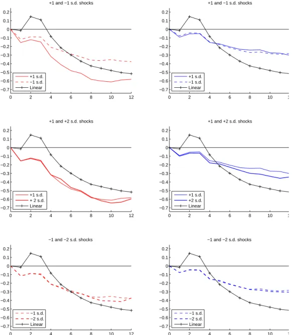
Figure 2.8 and Figure 2.9 present the impulse responses of the output and the price level
from the L2-STVAR using the fourth lag of the federal funds rate as the switching variable.
The estimated slope of transition function is 100, and the locater is (-0.7458,-0.7412).
The baseline responses of the output and the price level are slightly different from the ones
of M odelB. An increase in the federal funds rate decreases output immediately. Then the
effect dies down quickly up to the sixth quarter. The output is stable at about 0.7 percent
lower than the initial level. The size of shocks is 0.97 percent. So the policy targeting at the
interest rate policy is more effective than the one targeting at money supply. The responses
of price to policy shocks have similar pattern to the one of M odelB but it is less sensitive to
the shocks. It increases by 1.15 percent in 3 years. The fact that the price response is less
sensitive partially explains how output is more sensitive.
The same conclusions for the asymmetric effects can be drawn in this section. For the
output, the only apparent asymmetry is the responses to the shocks in the low and the high
growth periods. Again, the baseline VAR seems to be an average of the responses between
the two periods. Asymmetric responses to the different size of shocks are not found. However,
there are some evidences that the direction of the shocks has different effects. The output is less
sensitive to expansionary policies than contractionary policies in both low and high growth
periods. The response of the price level exhibits a price puzzle. The price level increases