PubMedCentral-PMC5764572.pdf

(1)

Competing interests:The authors declare that no competing interests exist.

Funding:See page 20

Received:30 September 2017 Accepted:22 December 2017 Published:11 January 2018

Reviewing editor: Andrea Musacchio, Max Planck Institute of Molecular Physiology, Germany

Copyright Suzuki et al. This article is distributed under the terms of theCreative Commons Attribution License,which permits unrestricted use and redistribution provided that the original author and source are credited.

An optimized method for 3D fluorescence

co-localization applied to human

kinetochore protein architecture

Aussie Suzuki*, Sarah K Long, Edward D Salmon

Department of Biology, University of North Carolina at Chapel Hill, Chapel Hill,

United States

Abstract

Two-color fluorescence co-localization in 3D (three-dimension) has the potential to achieve accurate measurements at the nanometer length scale. Here, we optimized a 3D

fluorescence co-localization method that uses mean values for chromatic aberration correction to yield the mean separation with~10 nm accuracy between green and red fluorescently labeled protein epitopes within single human kinetochores. Accuracy depended critically on achieving small standard deviations in fluorescence centroid determination, chromatic aberration across the measurement field, and coverslip thickness. Computer simulations showed that large standard deviations in these parameters significantly increase 3D measurements from their true values. Our 3D results show that at metaphase, the protein linkage between CENP-A within the inner

kinetochore and the microtubule-binding domain of the Ndc80 complex within the outer

kinetochore is on average~90 nm. The Ndc80 complex appears fully extended at metaphase and exhibits the same subunit structure in vivo as found in vitro by crystallography.

DOI: https://doi.org/10.7554/eLife.32418.001

Introduction

Confocal light microscopy (LM) is widely used for understanding protein localization, architecture, and functions in cells, but the maximum resolution without any image processing is still only~200 nm in the x-y image plane and~400 nm along the z-axis. The scale of many protein complexes is smaller than the diffraction limit of LM. In order to deduce the function of protein complexes, it is critical to develop a method to determine the three-dimensional (3D) locations of proteins within a complex in their native environment.

(2)

We previously reported a nm-scale map of how human kinetochore proteins are organized on average along the inner to outer kinetochore axis at metaphase, obtained using the ‘Delta’ two-color fluorescence co-localization method (Wan et al., 2009). The Delta method provided local chro-matic aberration (CA) correction in the x-y image plane by measurements along the K-K axis between pairs of sister kinetochores. More recently, Fuller and Straight (2012) developed a 3D method (termed CICADA [Co-localization and In-situ Correction of Aberration for Distance Analysis]) to measure the mean separation of red and green fluorescent centroids at individual kinetochores while locally correcting for CA in the x, y, and z directions using a third color (Fuller and Straight, 2012). Their method yielded an identical value to what was obtained by the Delta method (Fuller and Straight, 2012;Suzuki et al., 2014;Wan et al., 2009). In contrast, a recent report by Smith et al., 2016used a 3D measurement method to obtain mean separation values for protein domains within kinetochores that were significantly greater than our Delta values and the 3D value obtained by the CICADA method (Fuller and Straight, 2012; Smith et al., 2016; Suzuki et al., 2014;Wan et al., 2009). This group questioned the accuracy and significance of the Delta values because they were ‘1D measurements and neglected z-axis information’.

In this paper, we have tested the above conclusion by optimizing a 2D and 3D fluorescence co-localization method to obtain the mean separation between the centroids of green and red foci with ~10 nm accuracy (Figure 1). The method depends on correcting CA based on mean values from a fluorescent standard, a method commonly used for fluorescence co-localization, but not pre-viously optimized and rigorously analyzed for sources of error, as performed here. Computer simula-tions were used to understand how well the measurement method works and to find how accuracy is limited in our method. This study revealed major sources of error produced by standard deviations (SDs) in fluorescent centroid determination, CA correction, and coverslip thickness, as well as addressing several issues concerning fixation methods. We found that our 3D measurements applied to human kinetochores were similar to the Delta measurements and much shorter than those reported bySmith et al., 2016. Their larger measurements may be explained by much larger SDs in centroid determination and CA correction than typical of our experiments. We also used the known structure of the Ndc80 complex as a ‘Molecular Ruler’ to verify the accuracy of our measurement method, and to determine its subunit structure and conformation within the kinetochore.

Results

Principles of the method

Sample preparation

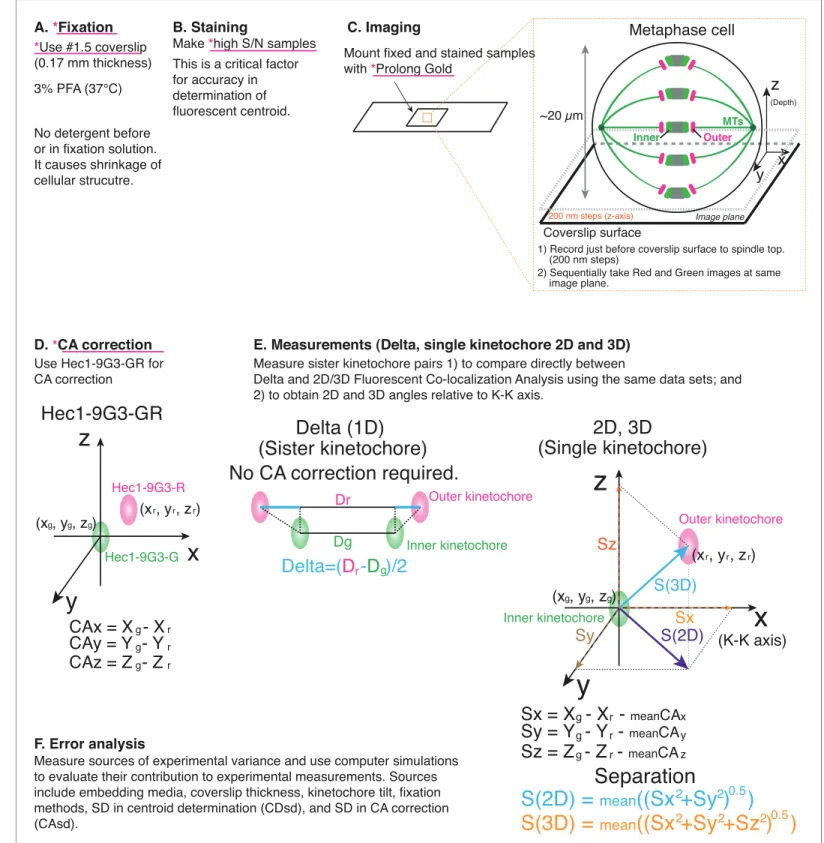
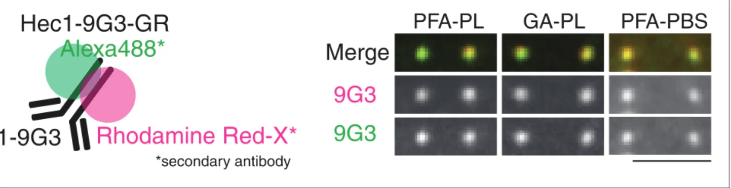
HeLa cells were grown on #1.5 coverslips, the design value for the microscope objective, to prevent Z-axis CA (chromatic aberration) (Figure 1A). Cells were fixed with paraformaldehyde (PFA) without pre-extraction or supplement of detergent in the PFA solution, and stained with primary antibodies using a protocol from previous studies (Figure 1A) (Suzuki et al., 2015; Suzuki et al., 2014; Suzuki et al., 2011). The concentration of green and red secondary antibodies was adjusted to give nearly equal fluorescence intensity (Figure 1B). Integrated kinetochore fluorescence above back-ground (>100,000 photon counts per kinetochore) was important to minimize the SD of centroid determination (CDsd) close to 5 nm (Thompson et al., 2002). Labeled samples were typically mounted with ProLong Gold mounting media. For the cellular CA correction standard, a monoclonal antibody (9G3) was used to label Hec1 (hsNdc80) protein at a site just inside of its MT binding CH domain, and this antibody was double labeled with green and red fluorescence by secondary anti-bodies (called Hec1-9G3-GR).

Imaging

(3)

Coverslip surface

y

z

200 nm steps (z-axis)

(Depth) Outer Inner

Metaphase cell

MTs Image plane

x

Mount fixed and stained samples with *Prolong Gold

A. *Fixation

No detergent before or in fixation solution. It causes shrinkage of cellular strucutre.

B. Staining

Make *high S/N samples This is a critical factor for accuracy in determination of fluorescent centroid.

C. Imaging

D. *CA correction

Dg

Delta=(

D

-

r

D

)/2

Dr

g

Delta (1D)

(Sister kinetochore)

CAx = X - X

CAy = Y - Y

CAz = Z - Z

g r

Hec1-9G3-GR

~20 µm

Use Hec1-9G3-GR for CA correction

Measure sources of experimental variance and use computer simulations to evaluate their contribution to experimental measurements. Sources include embedding media, coverslip thickness, kinetochore tilt, fixation methods, SD in centroid determination (CDsd), and SD in CA correction (CAsd).

F. Error analysis

S(2D) =

mean

((Sx +Sy ) )

2 2 0.5

S(3D) =

mean

((Sx +Sy +Sz ) )

2 2 20.5

Separation

Sx = X - X -

meanCA

Sy = Y - Y -

meanCA

Sz = Z - Z -

meanCA

g r g r g r x y z

x

z

y

(x , y , z )g g g

(x , y , z )r r r

Hec1-9G3-G

Hec1-9G3-R

x

z

y

(x , y , z )

g g g

Sz

Sx

Sy

S(2D)

S(3D)

(x , y , z )

r r r

2D, 3D

(Single kinetochore)

Inner kinetochore

Outer kinetochore

E. Measurements (Delta, single kinetochore 2D and 3D)

Measure sister kinetochore pairs 1) to compare directly between

Delta and 2D/3D Fluorescent Co-localization Analysis using the same data sets; and 2) to obtain 2D and 3D angles relative to K-K axis.

1) Record just before coverslip surface to spindle top. (200 nm steps)

2) Sequentially take Red and Green images at same image plane.

No CA correction required.

(K-K axis)

Inner kinetochore

Outer kinetochore

3% PFA (37℃)

*Use #1.5 coverslip (0.17 mm thickness)

Figure 1.Principle of procedure used in this study. (A) Fixation: 3% PFA in PHEM buffer without any detergent was used as standard fixation in this

study (Details in Text and Methods). (B) Staining: Fixed samples were immunofluorescently labeled with antibodies to enhance S/N. Samples were usually mounted with Prolong Gold. (C) Imaging was performed by spinning disk confocal microscopy (See Materials and methods for details). (D) For CA correction, Hec1-9G3 monoclonal antibody was labeled by green and red tagged secondary antibodies (Hec1-9G3-GR). (E) Measurements: X, Y, Z coordinates of the centroids of green and red kinetochore fluorescence were determined by 3D Gaussian fitting. Details of equations for separation measurements are in Text, Figures, and Methods. (F) Error analysis: computer simulations were used for error analysis of the method. The sources of potential errors in separation measurements were highlighted in pink underline with *.

(4)

Image analysis

We selected sister kinetochores for measurement not only for Delta values (Figure 1D–E), but also to obtain the direction of the sister-sister kinetochore axis (K-K). For each kinetochore, we obtained the x, y, z coordinates for the centroids of green (Xg, Yg, Zg) and red (Xr, Yr, Zr) using 3D Gaussian fitting methods (Wan et al., 2009). The Sx, Sy, and Sz coordinates of the separation vector S between green and red foci were calculated from Sx = Xg-Xr-meanCAx (CAmx), Sy = Yg-Yr-mean-CAy (CAmy), and Sz = Zg-Zr-meanCAz (CAmz) (Figure 1E), where the mean values of CAx, CAy, and CAz were obtained from kinetochores labeled with Hec1-9G3-GR within our measurement vol-ume (Figure 1D). ‘Raw’ values for the mean separation vector lengths in 2D and 3D were calculated for each pair of green-red kinetochore labels as S(2D) = mean ((Sx2 _{+ Sy}2₎0.5_{) and S(3D) = mean} ((Sx2 + Sy2 + Sz2)0.5) from measurements of 200 to 400 kinetochores obtained from 5 to 20 different cells (Figure 1E). The mean of these ‘raw’ separation values (S(2D), and S(3D)) were over-estimates (Churchman et al., 2006;Churchman et al., 2005). In order to obtain more accurate mean separa-tion values, a maximum likelihood method was applied to the raw separasepara-tion data (called ML2D and ML3D) (Churchman et al., 2006;Churchman et al., 2005).

Error analysis

Potential errors from different embedding media, the wrong coverslip thickness, kinetochore tilt, and different fixation methods were examined experimentally (Listed inFigure 1—source data 1). A computer simulation of the measurement method was used to evaluate the significance of these errors, as well as errors produced by the SDs in centroid determination (CDsd) and CA (CAsd) over the field of measurement (Figure 1F).

Chromatic aberration (CA) measurements from a cellular standard

CA within our measurement was determined from CAx = Xg-Xr, CAy = Yg-Yr, and CAz = Zg-Zr mea-sured for Hec1-9G3-GR labeled kinetochores of metaphase cells (Figures 1Dand2). The mean val-ues of CAx, CAy, and CAz plus their standard deviations (SDs) are listed in Table 1 for several different preparations. Note the mean values for CAx, CAy, and CAz were each very similar between different preparations. We included one preparation where the embedding solution was PBS. PBS has a refractive index near water, 1.33, and far from the refractive index of the coverslip (~1.52). The mean CAx, CAy, and CAz values were similar to those using the ProLong Gold embedding medium (Table 1). The major difference was a much larger SD for CAz compared to ProLong Gold (48 nm vs~18 nm,Table 1). This occurs because the lower refractive index induces spherical aberration that increases with z-axis depth from the coverslip surface (Figure 2—figure supplement 1). We also tested one sample with glutaraldehyde (GA) fixation and embedding with ProLong Gold. The mean CA values were nearly identical to the results obtained from PFA fixation (Table 1).

A small measurement region in the center of the camera detector (~300200 pixels) was used for

the entire analysis in this study (Figure 2—figure supplement 2A–B). In the measurement region, there was a gradient for CAx in the x direction (~30 nm/ 280 pixels (19mm)), but not in the y or z directions. There was a gradient for CAy in the y direction (~21 nm/180 pixels (11.5mm)), but not in the x or z directions. There was no noticeable gradient for CAz in either the x, y, or z directions com-pared to the SD (Figure 2—figure supplement 3). These gradients in CA had no more effect on measurement accuracy than randomly distributed CA values with the same mean and SD (see com-puter simulations below).

Figure 1 continued

The following source data is available for figure 1:

Source data 1.Pipeline for obtaining mean 3D separation measurements with nm-scale accuracy.

(5)

Validation of our 2D and 3D co-localization method for known

separations within the kinetochore

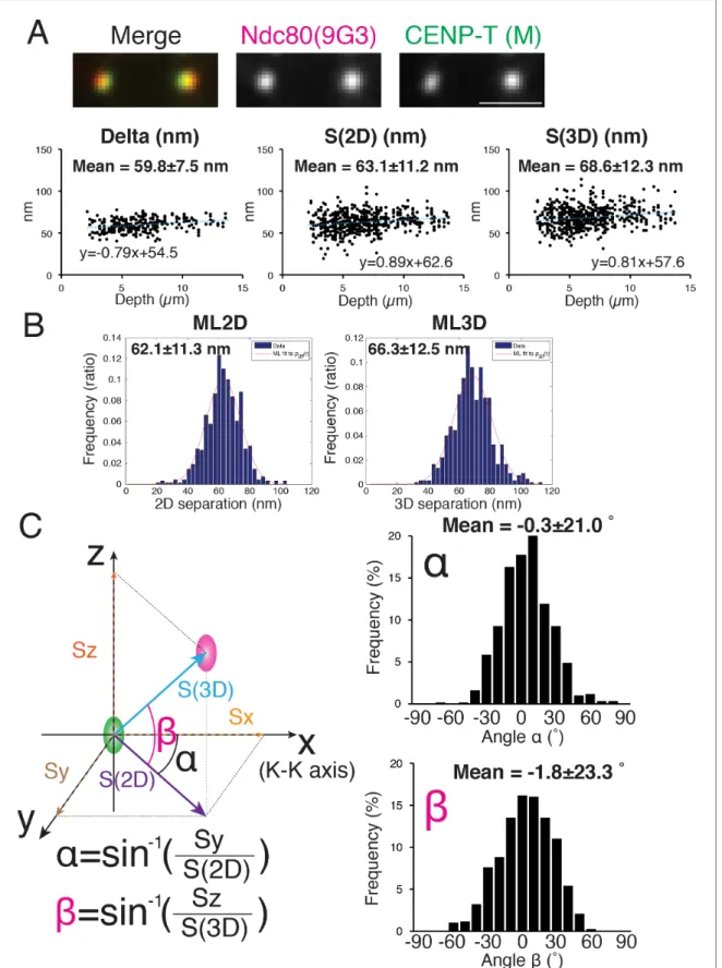
We initially measured the 2D and 3D separations between an antibody to CENP-T (CENP-T (M), Gascoigne et al., 2011) and Hec1-9G3 because previous studies reported values of Delta and 3D mean separations (by the CICADA method) using these same antibodies (Fuller and Straight, 2012; Suzuki et al., 2014;Wan et al., 2009). The reported 1D and 3D values for CENP-T (M) and Hec1-9G3 were~60 and~62 nm respectively. Our mean separation±SD between CENP-T (M) and Hec1-9G3 for Delta = 60±7.5 nm, S(2D)=63±11.2 nm, ML2D = 62±11.3 nm, S(3D)=69±12.3 nm, and

ML3D = 66±12.5 nm (Figure 3A–B), almost identical to the previous studies (Fuller and Straight, 2012;Suzuki et al., 2014;Wan et al., 2009).

The orientation of the separation vector at each kinetochore was also calculated relative to the K-K axis. For CENP-T(M) to Hec1-9G3, the mean vector angle to the K-K axis in the X-Y plane, angle a = 0.3 ± 20.1 degrees, while the mean vector angle relative to the Z-axis (angle b) was 1.8 ±23.3 degrees (Figure 3C). A significant fraction of the SD in these angles may be due to errors from CDsd and CAsd (see computer simulations below).

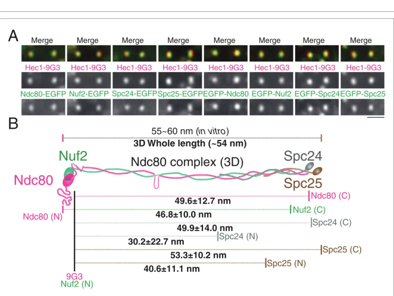
To further test the accuracy of our 2D/3D co-localization method, we examined the mean separa-tion of different domains within the Ndc80 complex. We chose the Ndc80 complex as a molecular ruler, since its protein structure is well known. The Ndc80 complex contains a dimer of Ndc80/Nuf2 and a dimer of Spc24/Spc25 (Cheeseman et al., 2006;Ciferri et al., 2008;Musacchio and Desai,

Merge

9G3

PFA-PL

GA-PL

PFA-PBS

Hec1-9G3-GR

*secondary antibody

Rhodamine Red-X*

Alexa488*

Hec1-9G3

Figure 2.CA (Chromatic aberration) measurements using Hec1-9G3-GR. Schematic model of Hec1-9G3-GR. Hec1-9G3 antibody was labeled by

secondary antibodies with Rhodamine Red-X and Alexa 488 (left). Representative Hec1-9G3-GR images in samples fixed by PFA or GA mounted with Prolong Gold or PBS.

The following figure supplements are available for figure 2:

Figure supplement 1.CAz is insensitive to depth in samples mounted with Prolong Gold, but not in samples mounted with PBS.

Figure supplement 2.Center of camera image was used for all analysis.

Figure supplement 3.Measurement of CA of the microscope optics.

Table 1.Mean and SD values of CAx, CAy, CAz for different sample preparations.

Fixation MM Green Red CAx (nm) CAy (nm) CAz (nm) N Use for correction PFA PL 9G3 9G3 13.1±9.1 15.8±7.5 3.5±17.6 166

PFA PL 9G3 9G3 14.7±11.4 13.2±12.1 1.5±17.0 256 PFA PL 9G3 9G3 15.7±12.5 15.6±8.2 4.8±20.2 206 Use for correction PFA PBS 9G3 9G3 13.2±10.7 18.7±10.4 2.7±47.5 168 Use for correction GA PL 9G3 9G3 19.2±10.3 16.0±9.0 6.8±18.8 170

(6)

Figure 3.Mean Delta, 2D, and 3D separations between Hec1-9G3 and CENP-T (M). (A) Representative immunofluorescent (IF) images (top) and plots of Depth verses Delta, S(2D) and S(3D) for the separation between CENP-T(M) and Hec1-9G3 (bottom). (B) Histograms of maximum likelihood fit used to calculate ML2D and ML3D. (C) Orientation of the S(3D) separation vector relative to the sister K-K axis (x-axis in this diagram). Angleais the rotation of the S(2D) vector component in the x-y plane away from the K-K (x-axis) and anglebis the rotation of the S(3D) vector away from the x-y plane and

(7)

2017). Most of the length of the Ndc80 complex is alpha helical coiled-coil, and its contour length is 55~60 nm, as measured in vitro by electron microscopy and crystallography (Ciferri et al., 2008; Huis In ’t Veld et al., 2016;Valverde et al., 2016;Wei et al., 2005). To reveal the cellular Ndc80 complex structure, we developed HeLa cells stably expressing Ndc80, Ndc80-EGFP, EGFP-Nuf2, Nuf2-EGFP, EGFP-Spc24, Spc24-EGFP, EGFP-Spc25, or Spc25-EGFP (Figure 4A).Figure 4B

Figure 3 continued

toward the z-axis (schematic on left). Histograms ofaandbvalues (Right). n > 600 individual kinetochores. All values were mean±SD. Note, CENP-T(M) is a polyclonal antibody against whole CENP-T protein, and its epitope is not precisely known (Gascoigne et al., 2011).

A

Ndc80

Nuf2

Spc25

Spc24

49.6±12.7 nm

9G3

Nuf2 (N)

Ndc80 (N)

Nuf2 (C)

Ndc80 (C)

Spc25 (C)

Spc24 (C)

3D Whole length (~54 nm)

46.8±10.0 nm

49.9±14.0 nm

Spc24 (N)

30.2±22.7 nm

53.3±10.2 nm

Spc25 (N)

40.6±11.1 nm

55~60 nm (

in vitro

₎

Ndc80 complex (3D)

B

Merge

Hec1-9G3

Ndc80-EGFP

Merge

Nuf2-EGFP

Merge

Spc24-EGFP

Merge

Spc25-EGFP

Merge

EGFP-Ndc80

Merge

EGFP-Nuf2

Merge

EGFP-Spc24

Merge

EGFP-Spc25

Hec1-9G3

Figure 4.2D/3D co-localization measurements of a structural standard, the extended Ndc80 complex. (A) Representative immunofluorescent images of

Hec1-9G3 and EGFP fused to different protein domains along the Ndc80 complex (See Text and Materials and methods). (B) Schematic summary of the ML3D Ndc80 complex measurements at metaphase. All values were mean±SD. n > 200 kinetochores for each measurement. Detail values are listed in

Figure 4—figure supplement 1.

The following source data and figure supplement are available for figure 4:

Source data 1.The list for Ndc80 complex measurements.

Figure supplement 1.Detailed sub-protein structure of Ndc80 complex.

(8)

andFigure 4—source data 1show the separation values relative to Hec1-9G3 to different ends of the Ndc80, Nuf2, Spc24, and Spc25 proteins, tagged in each case with EGFP. For example, the mean separation measurements between Spc25-EGFP and Hec1-9G3 were Delta = 49±5 nm, S(2D)

=52±10 nm, S(3D)=55±10 nm, ML2D = 51±10 nm, and ML3D = 53±10 nm. The Ndc80 complex

is likely extended along kMTs since the Delta and ML3D values for the length of the Ndc80 complex are nearly identical. Also, overall, our Delta, 2D, and 3D mean separation measurements yielded a close fit to a Ndc80 complex structure that was determined in vitro (Ciferri et al., 2008; Valverde et al., 2016). As expected, the C-terminus of Spc24 is located a few nm inside of the C-terminus of Spc25, and Spc24 is longer than Spc25 (Figure 4—figure supplement 1) (Valverde et al., 2016). The CH-domain of Nuf2 is located a few nm inside of the N-terminal CH domain of Ndc80, and Ndc80 is longer than Nuf2 (Figure 4—figure supplement 1) (Ciferri et al., 2008;Valverde et al., 2016). Unexpectedly, in vivo, the C-terminus of Ndc80 locates much closer to the globular domains of Spc24/Spc25 (Figure 4B). This difference might be caused by structural restrictions on the position of the EGFP tag, which was tethered to the protein end by a nine amino acid linker.

Sister kinetochore pairs were used for the majority of measurements in this study to directly com-pare separations obtained by Delta and 2D/3D fluorescent co-localization methods using the same data sets. To test if selection of sister pairs influenced our measurements, we measured 120 kineto-chores selected randomly in a single metaphase cell. This produced a mean separation value nearly identical to the mean value for single kinetochore measurements of sister pairs obtained from six metaphase cells (Table 2).

The mean human kinetochore protein architecture at metaphase

measured by the Delta method and our 3D method are similar

Figure 5shows how the centroids of protein labels are separated on average along the inner-outer kinetochore axis based on our 2D/Delta measurements (Top) and 3D measurements (bottom). All of our 2D and Delta values are nearly identical (usually less than 3 nm difference). In general, our 3D measurements were only~5 nm larger than the Delta or 2D values (Figure 5 and the Figure 5— source data 1). Unlike the 3D kinetochore protein architecture proposed by (Smith et al., 2016), our data showed no ~70 nm gap between CCAN protein domains and the Ndc80 complex. The inner kinetochore proteins are much closer to the outer kinetochore, corresponding to the previous studies using Delta measurements (Suzuki et al., 2014). For example, our 3D mean separation between CENP-A and Hec1-9G3 is ~90 nm, which is nearly identical to values obtained by Delta (~84 nm) and ML2D (~85 nm). InFigure 5, the Ndc80 complex and protein linkage to the inner kinet-ochore are shown aligned with the axis of kMTs because the ML3D mean separation values are only slightly greater than their corresponding Delta values, and the Delta value is a projection of the ML3D value along the K-K axis.

Coverslip thickness both greater and less than 0.17 mm produces z-axis

chromatic aberration (Z-offset) independent of focal depth

Normally the value of Z-offset (mean Sz) for each coverslip-slide preparation was within±25 nm of zero (Figure 5—source data 1). However, occasionally, significantly large positive or negative values occurred, which made the 3D measurement much larger than for small Z-offsets. The largest Z-offset occurred for one sample stained for CENP-T(M) and 9G3,~80 nm (Table 3A), which increased the S (3D) from 65 to 103 nm (Table 3A,). If this large Z-offset was subtracted from the Sz data, the mean zS3D (S(3D) with subtracted Z-offset) value became close to the value with near zero Z-offset,~65 nm (Table 3A). This comparison indicated that the higher Z-offset was independent of the actual

Table 2.Comparison of measurements for kinetochores that were part of sister pairs and kinetochores selected at random from a single metaphase cell.

Methods Green Red Delta (nm) S(2D) (nm) S(3D) (nm) ML2D (nm) ML3D (nm) n

Sister pair Spc25-EGFP 9G3 49.4±4.6 51.5±9.6 55.2±10.0 50.6±9.7 53.3±10.2 280 (140 pairs) from 6 cells Random Spc25-EGFP 9G3 N.A. 50.8±6.7 55.3±7.7 50.3±6.7 54.2±7.8 120 from single cell

(9)

Figure 5.Schematic core-kinetochore drawing measured by 2D/Delta or 3D co-localization method. Schematic picture of the mean positions of protein labels within the core kinetochore protein architecture measured using ML2D/Delta (top) and ML3D (bottom) methods. N or C are the mean positions of N-terminal or C-terminal EGFP fusions or specific antibodies. M indicates the mean position measured using polyclonal antibodies whose epitope(s) are not precisely known.

(10)

mean separation between green and red labels. This comparison also indicated that there was some-thing about specimen preparation causing variation in z-axis CA.

To explore possible optical factors, we used a mathematical analysis reported previously (Gibson and Lanni, 1992). This analysis calculates, relative to the design values for the objective, changes in optical path for light coming from a fluorescent point as a function of the refractive index and thickness of the specimen media, the coverslip thickness, and immersion oil, as well as wave-length. It showed that the amount of z-axis CA is highly sensitive to changes in the thickness of the coverslip. We tested this possibility by using different thickness of coverslips. We did most of our experiments reported in this paper using # 1.5 coverslips. We measured their thickness with a micrometer, and the mean value was 0.17 mm with a range of 0.16 to 0.19 (Figure 6, n > 100). For #1 coverslips, the mean was 0.15 mm and for #2 coverslips it was 0.22 mm (Figure 6). The mean Sz (Z-offset) for CENP-T(M) to Hec1-9G3 showed~±10 nm for #1.5 coverslips, 29 to 19 nm for #1 coverslips, and 29 to 46 nm for # 2 (Table 3B). The plot inFigure 6—figure supplement 1illustrates the sensitivity of Z-offset to coverslip thickness. A steep slope is seen when measured Z-offset values inTable 3Bare plotted as a function of the mean thickness we measured for #1, #1.5 and #2 cover-slips. Based on these experimental results, we suspect that unusually large Z-offset values (>25 nm) measured in our experiments (Figure 5—source data 1) were largely produced by coverslip thick-nesses much thinner or thicker than 0.17 mm.

In our study, we were careful to include similar numbers of kinetochores above and below the spindle equator. This is because kinetochores and their kMTs become tilted progressively with their radial distance away from the spindle axis (Figure 6—figure supplement 2A) (Smith et al., 2016; Wan et al., 2009). Both the inner and outer domains of metaphase kinetochores typically have their faces perpendicular to their kMTs (Wan et al., 2009). If kinetochores are only measured on the bot-tom half of the spindle, the mean value of Sz will not be zero because the upward kinetochore tilt in the lower half spindle is not canceled by the downward tilt from kinetochores in the upper half-spin-dle (Figure 6—figure supplement 2A–B). This kinetochore tilt had no effect on measured 3D mean separation since values from only kinetochores in the upper half of the spindle yielded similar results

Figure 5 continued

The following source data is available for figure 5:

Source data 1.List for core-kinetochore protein measurements.

Source data 2.List of primary antibodies.

Table 3.(A) List of Delta, S(2D), S(3D), Z-offset, and zS(3D) (Z-offset subtracted) for the mean separation between CENP-T(M) and Hec1(9G3) in samples with or without large Z-offset.

(B) List of Delta, S(2D), S(3D), Z-offset, and zS(3D) in samples with #1, #1.5, and #2 coverslips. The value zS(3D) was calculated from the

S(3D) data after subtraction of the mean Z-offset in the middle of the spindle from the Sz values. All values were mean±SD.

A Green Red Delta nm) S(2D)(nm) S(3D) (nm) Z-offset (nm) zS(3D) (nm) Example 1 CENP-T (M) 9 G3 59.5±6.3 60.8±8.8 102.4±26.7 79.7±32.9 68.9±10.2 Example 2 CENP-T (M) 9 G3 57.3±7.3 60.1±11.7 64.8±11.3 6.9±23.2 64.5±10.8

B Thickness Green Red Delta nm) S(2D)(nm) S(3D) (nm) Z-offset (nm) zS(3D) (nm)

Experiment 1 #1 CENP-T (M) 9 G3 60.4±6.9 63.5±12.4 75.2±17.6 28.6±31.1 70.4±14.2 Experiment 2 #1 CENP-T (M) 9 G3 59.2±10.0 62.6±11.7 72.6±16.3 18.3±33.9 70.6±14.6 Experiment 1 #1.5 CENP-T (M) 9 G3 57.3±7.3 60.1±11.6 64.8.±11.3 6.9±23.2 64.5±10.8 Experiment 2 #1.5 CENP-T (M) 9 G3 57.0±7.1 60.6±11.1 64.0±11.6 6.0±20.0 63.8±11.2 Experiment 1 #2 CENP-T (M) 9 G3 59.6±7.7 62.1±11.9 82.1±27.2 46.4±36.4 69.6±21.9 Experiment 2 #2 CENP-T (M) 9 G3 59.8±7.4 62.5±10.9 74.2±16.2 28.7±30.2 69.4±10.8

(11)

as from kinetochores in the lower half of the spindle (data not shown). Unlike 3D separation, the mean tilt angle b (but not angle a) was sensitive to unequal numbers of kinetochores above and below the spindle equator. The mean anglebis near zero in the middle of the spindle and reaches mean values of about 20–25 degrees at the bottom and top of the spindle (Figure 6—figure supple-ment 2C–D).

PFA fixation does not cause shrinkage, but pre-extraction or detergent

in PFA solution causes shrinkage of cellular structure

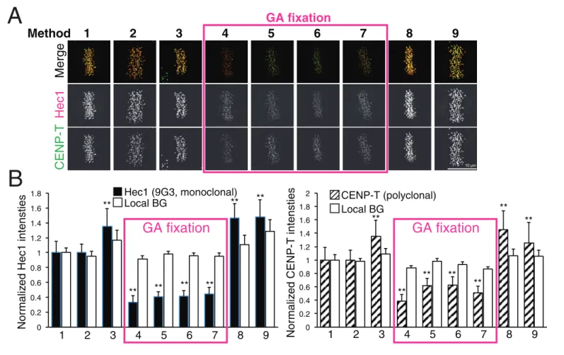
A recent study raised the issue that PFA fixation induced shrinkages compared to GA fixation (Magidson et al., 2016). GA has two aldehyde radicals and provides more robust fixation compared to PFA fixation. Because of this reason, GA fixation is usually used for electron microscopy. On the other hand, GA fixation exhibits strong auto fluorescence, and induces significantly less reactivity between cellular antigen and antibodies compared to PFA fixation. For immunofluorescence, a non-ionic detergent, such as Triton-X 100 or NP40, is often used to improve antibody penetration into the cell before, with, or after fixation. It is uncertain how these pre-permeabilization processes affect cellular architecture. For example,Magidson et al. (2016)concluded PFA fixation causes shrinkage. However, they actually supplemented 1% Triton-X 100 in their PFA fixation solution. Our standard method was primary fixation by PFA without detergent (Method one inTable 4), a method signifi-cantly different than the PFA fixation method used by (Magidson et al., 2016).

To test the effect of fixation and detergent for antibody reaction and separation measurements, we tested nine different fixation methods (Table 4, and Materials and methods). We used CENP-T (M) and Hec1-9G3 antibodies for this comparison (Figure 7A). These antibodies were the exact same antibodies used inFigure 3 in this study, and in previous reports (Fuller and Straight, 2012; Magidson et al., 2016;Suzuki et al., 2014;Wan et al., 2009). We first compared CENP-T(M) and Hec1-9G3 signal levels at kinetochores in the different methods (Figure 7B). Interestingly, both CENP-T(M) and Hec1-9G3 signal levels in GA fixation samples (Methods 4–7) were significantly reduced by~35% to 60% compared to PFA fixation (Method 1), PFA with detergent fixation (by 20– 30%), or MeOH fixation (~20%) (Figure 7B). However, local background levels (surrounding area of kinetochore) were not significantly different between all fixation methods, indicating that GA fixation significantly reduced the signal to noise ratio (S/N) compared to PFA or MeOH fixation (Figure 7B).

Next, we measured mean separation between CENP-T(M) and Hec1-9G3. Surprisingly, we could not find any significant differences between PFA fixation (Methods 1–2) and GA fixation (Methods 4–7). However, we observed significant shrinkage when samples were fixed by Methods 3, 8, and 9

0 10 20 30 40 50

0.18 0.19 0.2 0.21 0.22 0.23 0.24 0

10 20 30 40 50 60 70

0.15 0.16 0.17 0.18 0.19 0.2 0

10 20 30 40 50 60

0.12 0.13 0.14 0.15 0.16 0.17

Thickness (µm)

Coverslip (#1)

Coverslip (#1.5)

Coverslip (#2)

Mean = 0.15 Range: 0.14~0.16

Mean = 0.17 Range: 0.16~0.19

Mean = 0.22 Range: 0.19~0.23

F

requency

(%)

F

requency

(%)

F

requency

(%)

Figure 6.Accuracy of separation measurements depends critically on mean z-axis CA (Z-offset) produced by coverslip thickness variations from

standard value. Measured variability of coverslip thickness within #1, #1.5, and #2 coverslips.

The following figure supplements are available for figure 6:

Figure supplement 1.Z-offset changes dependent on coverslip thickness.

Figure supplement 2.Z-axis offset from kinetochore tilt.

(12)

(Table 5). Interestingly, we could not see any shrinkage when we fixed by GA with Triton X-100, Tri-ton X-100 treatment before GA or GA/PFA (Methods 5–7). Although there are no differences between PFA and GA fixation for the separation between CENP-T(M) and Hec1-9G3, we found that pre-extraction by Triton X-100 or PFA fixation with Triton X-100 induced significant shrinkage com-pared to GA with Triton X-100. This result is consistent with the report ofMagidson et al. (2016). However, our standard PFA fixation method (Method 1) did not produce any shrinkage.

Computer simulations for understanding the method and its limitations

The method using mean values of CA to correct chromatic aberration is widely used, but the limita-tions of this method are not well established. We evaluated the method by computer simulalimita-tions. Critical factors are SDs of centroid determination (CDsd) and CA (CAsd). In our simulations, kineto-chores were located at 10 pixel intervals in both the X and Y axis directions for the typical image region of 0–280 pixels in the X- direction and 0 to 190 pixels in the Y-direction (Figure 8). At each kinetochore position (p), the separation vector extended from the origin to a length S in the x direc-tion. The green (Xgp, Ygp, Zgp) values at the origin had a mean of zero plus a CDsd determined by sampling CDsd times a normalized random number for the x, y, and z directions (Figure 8). The red (Xrp, Yrp, Zrp) values included S in the x-direction and Z-offset in the Z direction. They also included a value for the CA at each kinetochore position, CAp, plus CDsd for each direction (Figure 8). Two methods were used to generate the CAp values. In the first, for each x, y, and z direction, CAp was calculated from the measured mean CA plus the CAsd times a normalized random number. In the second, CAp for the x and y directions were calculated from least square fits to the CA cellular data because of the 30 nm and 20 nm decrease respectively across the measurement field (Figure 2—fig-ure supplement 3). However, this second procedure gave identical results as the first method out-lined inFigure 8, which is the CA correction method we used experimentally. Mean and SD values for S(2D), S(3D), ML2D, ML3D, anglea, and anglebwere calculated using the same equations as we did in analysis of cellular data (Figures 1Eand3C).

Table 4.Summary of fixation methods used inFigure 7.

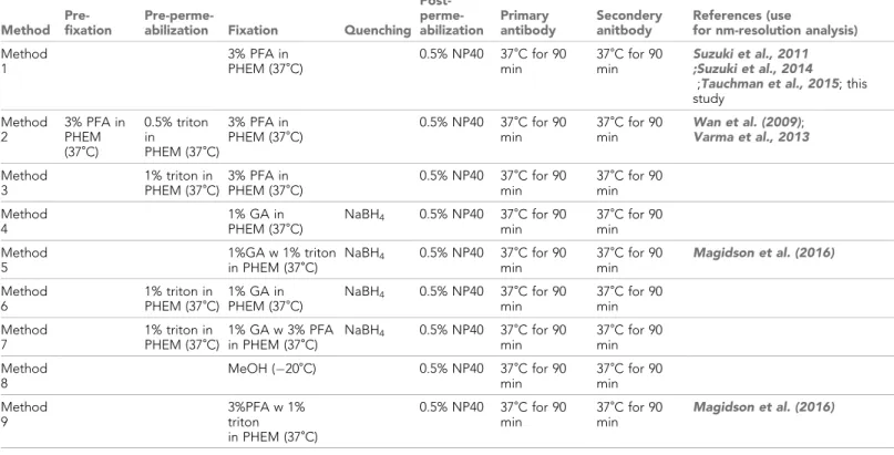
Detailed protocols for the different fixation methods used inFigure 7. Method 1 is the protocol used in this study.

Method Pre-fixation

Pre-perme-abilization Fixation Quenching Post- perme-abilization Primary antibody Secondery anitbody References (use

for nm-resolution analysis) Method

C)

NaBH4 0.5% NP40 37

˚

C for 90

min

37

_˚

C for 90 min

Magidson et al. (2016)

Method 6

_˚

C)

1% GA in PHEM (37

_˚

C)

NaBH4 0.5% NP40 37

˚

C for 90

min

37

_˚

C for 90 min Method

7

_˚

C)

1% GA w 3% PFA in PHEM (37

C) 0.5% NP40 37

_˚

C for 90 min

37

_˚

C for 90 min Method

9

2

3

4

5

6

7

8

9

0 0.2 0.4 0.6 0.8 1 1.2 1.4 1.6 1.8

1

2

3

4

5

6

7

8

9 Nor

maliz

ed Hec1 intensties

Nor

mali

z

ed CENP-T intensties

1

2

3

4

5

6

7

8 Merge

Hec1

CENP-T

Hec1 (9G3, monoclonal)

Local BG CENP-T (polyclonal) Local BG

10 µm

9 GA fixation

GA fixation

A

B

**

** ** ** **

** **

**

** ** **

**

** _**

Method

Figure 7.Comparison of various fixation methods for signal intensity and mean fluorescence co-localization analysis. (A) Representative

immunofluorescent images stained by CENP-T(M) and Hec1-9G3 antibodies using the fixation protocols listed inTable 4. (B) The plots of normalized signal intensity of Hec1-9G3 (left) and CENP-T (right) at kinetochores using the fixation protocols listed inTable 4. The signal intensities were normalized for the mean values of PFA fixation (~20,000 integrated fluorescence counts above local background for Method 1). All values were mean±SD. n > 200 individual kinetochores for each experiment. **p<0.05 (t-test).

(14)

in the anglesaandbare largest for small separations (Table 6B). For example, they were 9 and 19 degrees (S = 60 nm) or 6 and 11 degrees (S = 100 nm). These results indicate that our CDsd and CAsd caused about half to two-thirds of the SD measured in cells for separations of 60 nm (SDs of anglesa andb were 21 and 23 degrees, respectively; CENP-T-Hec1-9G3 in Figure 3C) or 90 nm

Table 5.The list of measured values for Delta, ML2D, ML3D, dDelta, dML2D, and dML3D using protocols inTable 4.

The dDelta, dML2D, dML3D were differences from Method 1 (PFA fixation). All values were mean±SD. n > 200 individual kinetochores

for each experiment.

Red-Green = mean±S.D. nm

Delta (nm) ML2D (nm) ML3D (nm) dDelta (nm) dML2D (nm) dML3D (nm)

Method 1 57.2±7.3 59.1±11.6 62.6±11.5 0 0 0.0

Method 2 56.8±6.0 58.6±8.8 61.3±8.6 0.4 0.5 1.3

Method 3 50.1±7.1 52.8±8.5 56.4±8.2 7.1 6.3 6.2

Method 4 58.7±9.1 61.5±12.4 63.1±22.9 1.5 2.4 0.5 Method 5 55.2±8.9 56.9±11.7 61.3±15.5 -2 2.2 1.3 Method 6 57.2±9.0 60.0±12.9 63.5±21.6 0 0.9 0.9 Method 7 54.0±10.0 57.2±12.1 57.7±12.2 3.2 1.9 4.9 Method 8 46.4±5.3 48.3±7.7 52.0±7.7 10.8 10.8 10.6 Method 9 51.8±7.4 53.8±9.7 56.7±10.0 5.4 5.3 5.9

CDsd: SD of centroid determination (x, y, z) = (± CDsdx, ± CDsdy, ± CDsdz) CAsd: SD of CA (x, y, z) = (± CAsdx, ± CAsdy, ± CAsdz)

randn: a normalized random number with mean = 0

CApx = mean CAx (CAmx) + CAsdx*randn CApy = mean CAy (CAmy) + CAsdy*randn CApz = mean CAz (CAmz) + CAsdz*randn

p: each kinetochore x, y position in kinetochore array

. . . . . . . . .

. . . . . . . .

S

(Xgp, Ygp, Zgp)

= (0+CDsdxrandn, 0+CDsdyrandn, 0+CDsdz*randn)

Each kinetochore

1 2 3 4 5 6 ... 28 29 1

2

3

4

5

6

...

18 7

8

X (Nx)

Y

(Ny)

(Xrp, Yrp, Zrp) = (S+CApx+CDsdx*randn,

0+CApy+CDsdy*randn,

Z-offset+CApz+CDsdz*randn)

x

y

z

Kinetochore position (p) array

Figure 8.Diagram of simulation model. We used a 290180 pixel region (x and y) and kinetochores at positions (p) separated by 10 pixels in each

direction. All simulated values S(2D), S(3D), anglea, and anglebwere averaged from 2918 = 551 kinetochores. The maximum likelihood fit was

applied to the raw simulated S(2D) and S(3D) values in the same way as for the experimental analysis in this study.

(15)

(SDs of anglesaandbwere 16 and 22 degrees, respectively; CENP-A-Hec1-9G3 inFigure 6—figure supplement 2C–D). These simulations also showed that our SDs inhibit maximum likelihood fit below S =~18 nm (Table 6B). These simulation results indicate that much of our measured SD in the cell is not caused by variability between different kinetochores, but by the SDs in centroid measure-ment and CA correction.

Discussion

There are several key factors that influence the accuracy of the 3D fluorescence co-localization method we used for determining mean separation distances (all factors we identified are listed in Figure 1—source data 1). High S/N and bright specimens are needed for small CDsd. The measure-ment field should be restricted in area to keep the CAsd small. The correct coverslip thickness should be used to prevent Z-offset. These procedures are important because computer simulations show that mean 2D/3D separations and SDs in angles (aandb) all increase from their true values as a power function of the magnitudes of CDsd, CAsd, and Z-offset (Figure 9A–C). In addition, the use of the maximum likelihood method corrects the overestimate of mean separations obtained from S (2D) and S(3D) (Churchman et al., 2005).

Z-offset is a major source of error only if it is not produced by the specimen. As a general rule, we do not recommend subtracting Z-offset from Sz data since there could be a specimen contribu-tion. When using our method, we recommend repeating the specimen measurement with a 0.17 mm coverslip if Z-offset is larger than±25 nm to make sure there is not an unknown specimen contri-bution. Computer simulations of the measurement method showed that only absolute values of Z-offset >30 nm make 3D mean separation measurements significantly larger (Figure 9C). Also, our method produces nearly identical results from multiple samples.Figure 5—source data 1has meas-urements between CENP-A and Hec1-9G3 from four different coverslip preparations. Their Z-offsets varied between 17 and 4.4 nm, while their ML3D mean values varied between 86 and 93 nm.

Smith et al., 2016 reported that the mean 3D separation between endogenous CENP-A and the C-terminus of Ndc80 was 81.7±0.7 nm SEM (n = 3302, SD =±40 nm), about 42 nm larger than our measured value of 40 nm±~10 nm (SD) (Table 7).Table 7also provides three more examples showing differences of 24 nm to 60 nm between their and our mean 3D separation measurements.

Table 6.Computer simulations to determine measurement SD and to test the accuracy of using mean CA for CA correction.

(A) Comparison of~60 nm experimental results to simulated results for a fixed S value of 60 nm, the estimated CDsd for our

measure-ments, and with or without CAsd. (B) Simulated S(3D), and ML3D values for different input S values with fixed angles (0˚), CDsd (x, y, z)

= (±4,±4,±8) and CAsd (x, y, z) = (±9.1,±7.5,±17.6). All simulated values were mean±SD.

A Delta (nm) S(2D) (nm) S(3D) (nm) ML2D (nm) ML3D (nm) a(

_˚

) b(

_˚

) Experiment CENP-T(M)-Hec1-9G3 60±7.5 63.1±11 68.6±12.3 62.1±11.3 66.3±12.3 0.3±21 1.8±23 Simulation (S = 60 nm) SDc (x, y,z) = (±4,±4,±8)

No CAsd 60.4±5.7 61.5±5.8 60.4±5.7 61.5±5.8 0.1±5.4 0±10.7 CAsd (x, y, z) = (±9.1,±7.5,±17.6) N/A 60.7±10.9 64.5±11.3 59.7±11 62.3±11.5 0.2±9.4 0.1±19.4

B input values simulation results

S±0 nm a(±0˚) b(±0˚) a˚ b˚ S(3D) (nm) ML3D (nm) 0 0 0 0.3±51.2 1.8±51.8 22±10.5 0±14.1 10 0 0 2.4±44.8 3.2±48.8 24.6±10.9 0±15.5 15 0 0 1.1±36 0.6±43.5 26.5±11.1 0±16.6

20 0 0 0.9±30.9 2.4±40.3 29.5±11.4 20.7±13.8 40 0 0 0.8±14.8 0.3±27.2 47±12.3 43.1±12.9 60 0 0 0.1±9.1 0.5±19.3 63.9±11.4 61.8±11.5 80 0 0 0.1±6.6 1±14.3 83.1±11.2 81.6±11.3 100 0 0 0.2±5.5 0.3±11.4 102.9±11.1 101.7±11.1

(16)

SinceSmith et al., 2016used mean CA values for CA correction as we did in this study, we investi-gated the possibility that significantly higher CDsd and CAsd compared to our values might be responsible for their larger 3D separation values. We estimated the CDsd from the SD of their Delta measurements for CENP-A to Spc24, which was~35 nm, compared to our value of 6 nm (Figure 9— source data 1) (Smith et al., 2016;Suzuki et al., 2014). This analysis yielded values for CDsd about five times larger than ours (22 nm, 22 nm, and 44 nm compared to 4 nm, 4 nm and 8 nm in the x, y

0 20 40 60 80 100 120

0 10 20 30 40 50 60 70 80 90 100 30 40 50 60 70 80 90 100 0 5 10 15 20 25 30 35 40 45 0 25 50 75 100 125 150

S(3D) (nm)

A

44 nm

68 nm

S = 40 nm separation Z-offset = 0

Input

2 3 4 5 6 7 8

1 9 10 11 12

a =

CAsd (x, y, z) = (±3a, ±3a, ±6a)

S(3D) (nm)

Z-offset (nm)

B

6'RIDQJOHњDQGћÝ

2 3 4 5 6 7 8

1 9 10 11 12

a =

Ý

C

Figure 9

Input S values

(40 nm) (60 nm) (70 nm)

Simulated 3D separation (nm)

(4, 4, 8), (9.1, 7.5, 17.6)

CDsd (x, y, z), CAsd (x, y, z)

(22, 22, 44), (25.5, 23.1, 43)

D

E

(23 nm)

-60

-40 -20 0 20 40 60

њDQGћDQJOHÝ

Alpha

Beta

CAsd (x, y, z) = (±3a, ±3a, ±6a)

(4, 4, 8), (9.1, 7.5, 17.6) (22, 22, 44), (25.5, 23.1, 43)

CDsd (x, y, z), CAsd (x, y, z) 0

$QJOHњ $QJOHћ

0

S = 40 nm separation

CAsd (x, y, z) = (± 9.1, ± 7.5, ± 17.6) CDsd (x, y, z) = (± 4, ± 4, ± 8) Input

Figure 9.Origins of error in mean separation measurements and comparison of our results to previous reports. (A) Plots of simulated S(3D) for 40 nm

separation with increasing values of CAsd (SD of CA) where the mean CA values were held constant at our measured values of 13.1, 15.8, and 3.5 nm respectively. Grey dashed line is nearly identical to the CAsd for our measurements and the red dashed line is nearly identical to the CAsd for the

Smith et al., 2016measurements. (B) Plots of SD of simulated angleaandbfor 60 nm separation using the same condition in (A). (C) Plots of simulated S(3D) for S = 40 nm separation for increasing values of Z-offset and the CAsd reported bySmith et al. (2016). (D) The simulated 3D separation using our SDs (black bars) or inSmith et al. (2016)(white bars). The true separations (S values) are 40, 60, 70, and 23 nm from left to right, which correspond to the mean values from Delta analysis inTable 7. (E) The simulated mean angleaandbwith±SD for the conditions in (E). Note, the input mean angleaandbwere zero, and S = 60 nm.

The following source data and figure supplement are available for figure 9:

Source data 1.Estimation of SD for centroid determination (CDsd).

Source data 2.Estimation of kinetochore-kinetochore variability (Ksd) in our measurements.

Figure supplement 1.About 10~15 kinetochore measurements are sufficient to obtain a mean value close to the mean separation values±SD

from>200 kinetochores.

(17)

and z directions) (Figure 9—source data 1). Such high CDsd values could explain why their Delta measurements are significantly larger than ours (Figure 9—source data 1). Their reported CAsd was also significantly larger than ours (26 nm, 23 nm and 43 nm compared to 9 nm, 7.5 nm and 18 nm in the x, y and z directions) (Smith et al., 2016). Results of simulations inFigure 9Dusing the values we estimated for their CDsd and their reported CAsd produce results nearly identical to their mean separation measurements, and show how the differences in the SDs between their and our measure-ments could be responsible for their much larger values. In addition, the higher levels for CDsd and CAsd are likely responsible for the very large SDs they measured for the anglesaandbcompared to ours (Figure 9E). In our measurements, large values of Z-offset were rare (Figure 5—source data 1); we have no information to judge how much other sources of error like Z-offset, contributed to theSmith et al. (2016)measurements.

Human kinetochores are built from multiple copies of core-kinetochore proteins (Suzuki et al., 2015). A previous study has shown that the accuracy of separation measurements is sensitive to the spatial staggering of the labeled molecules along the kinetochore inner to outer axis only for stagger greater than 200 nm, which has the possibility of producing two fluorescent peaks instead of a single peak if staggering is not random (Joglekar et al., 2009). All kinetochores labeled by specific anti-bodies or EGFP in our study exhibited a Gaussian distribution with a single peak. This indicates that our centroid measurements correspond to the mean position of the fluorescently labeled protein epitopes within human kinetochores.

Magidson et al. (2016)questioned whether the mean separation measurements averaged from multiple kinetochores (typically 200–400 kinetochores from 5 to 20 cells in our study) hide variation in the position of proteins relative to each other between different kinetochores (Magidson et al., 2016). We tried to address this question in several ways. First, we found that mean measurements of individual kinetochores (not sister pairs) within a single cell yielded the identical value at meta-phase as the mean obtained from kinetochores (sister pairs) within six different cells (Table 2). Thus, variations between cells or selected kinetochore measurements like in the Delta analysis is not an issue. Second, as expected for the Gaussian distribution measured for separation values (e.g. Figure 3B), we found that only 10–15 kinetochores were needed to be averaged to achieve the mean and SD typical of >150 kinetochores (Figure 9—figure supplement 1). Third, the SD of our 2D/3D measurements are small, typically less than 12 nm, and a significant part of this SD must be from the CDsd and CAsd (Table 6Aand see above discussion) and not from differences between kinetochores. To see this more clearly, we used the same simulations as in Figures 8–9 but with mean kinetochore-to-kinetochore variability (Ksd =±0,±5,±10, or±15 nm) (Figure 9—source data

2). Simulation results showed that Ksd of about ±5 nm or less plus measurement CDsd and CAsd

yielded the experimental mean SD value of 12.5 nm (Figure 9—source data 2). These results imply that the vast majority of kinetochores at metaphase have a similar protein architecture.

We found that our PFA fixation does not shrink kinetochore structure and produces exactly the same Delta, 2D, and 3D mean separation values obtained by the GA fixation. A major problem with GA fixation is that it interferes with antibody labeling, preventing immunofluorescence with many

Table 7.List of four examples of Delta and 3D mean separation measurements with±SD from this study andSmith et al., 2016.

Delta (Mean±SD nm) 3D separation (Mean±SD nm)

1 Smith et al., 2016 EGFP-CENP-A Ndc80(C-term) 58±35(n = 1002,±1.1 (SE)) 98±58(n = 4291,±0.9 (SE))

Smith et al., 2016 endogeous CENP-A Ndc80(C-term) N/A 84±40(n = 3302,±0.7 (SE)) This study endogeous CENP-A CENP-T (N-term) 40±6(n = 110) 46±12(n = 220)

2 Smith et al., 2016 endogenous CENP-C Ndc80 (N-term) N/A 103±74(n = 7476,±0.8 (SE)) This study endogenous CENP-C Hec1-9G3 58±5(n = 62) 67±8(n = 124)

3 Smith et al., 2016 EGFP-CENP-C Ndc80 (N-term) N/A 101±76(n = 1769,±1.8 (SE)) This study EGFP-CENP-C Hec1-9G3 69±9(n = 102) 77±15(n = 124)

4 Smith et al., 2016 EGFP-CENP-O Ndc80(C-term) N/A 81±52(n = 1881,±1.2 (SE)) This study EGFP-CENP-O Ndc80(C-term) 23±11(n = 97)* 21±16(n = 194)*

*These values were caliculated by (EGFP-CENP-O - Hec1-9G3) minus (Ndc80-EGFP - Hec1-9G3).

(18)

antibodies, and reduced fluorescence for others like those used inFigure 7. In addition, our data indicate that primary GA fixation may not be suitable for analysis of molecular distribution by immuno-electron microscopy because of poor recognition by antibodies. For immuno-electron microscopy, GA fixation should be used as the post-fixation solution, but only after the antibody reaction has been performed.

This study provides an optimized 3D fluorescence co-localization method with error analysis. It can achieve~10 nm accuracy for mean separations larger than 18 nm. Our mean 3D fluorescence co-localization measurements for human kinetochore protein architecture are close to the mean val-ues obtained using local correction of CA (Wan et al., 2009;Fuller and Straight, 2012) and suc-cessfully predict the known structural lengths of the Ndc80 complex components (Ciferri et al., 2008; Valverde et al., 2016; Musacchio and Desai, 2017). This optimized 3D co-localization method is a useful tool for broad research fields that need to determine mean protein architecture with nm-accuracy.

Materials and methods

Cell culture

HeLa cells were cultured in Dulbecco’s modified Eagle’s medium (Gibco) supplemented with 10% fetal bovine serum (Sigma), 100 U/ml penicillin and 100 mg/ml streptomycin at 37 ˚C in a humidified atmosphere with 5% CO2(Suzuki et al., 2015). siRNA resistance Ndc80, Ndc80-EGFP, EGFP-Nuf2, Nuf2-EGFP, EGFP-Spc24, Spc24-EGFP, EGFP-Spc25, and Spc25-EGFP constructs were linear-ized by restriction enzymes, and then purified plasmids were transfected using Effectene regents (Qiagen) according to the manufacturer’s instruction. The transfected cells were selected by Geneti-cin (Invitrogen) 48 hr after transfection. We collected more than 20 individual positive colonies from each transfection, then we tested expression levels of EGFP-tagged proteins by immunofluores-cence. We selected cell lines expressing EGFP-fusion protein at a similar level to the endogenous protein, as measured by immunofluorescence stained kinetochores using Spc24 and Hec1-9G3 anti-bodies. Other EGFP strains were described in a previous study (Suzuki et al., 2015;Suzuki et al., 2014). All cells were monoclonal cell lines. RNAi experiments were conducted using LipofectamineR-NAi MAX (Invitrogen) according to the manufacturer’s instructions. siRNA was performed with 100 nM of siRNA duplex and siRNA sequences of CENP-T, CENP-C, Ndc80, and Nuf2 were described previously (DeLuca et al., 2002;Suzuki et al., 2015). Sequences for Spc24 (GGUCGACGAGGA-CACGACA), Spc25 (CUGCAAAUAUCCAGGAUCU), and Nuf2 (GAAGUCAUGUAUCCACAUU) were used. The efficiency for depletion of CENP-T, CENP-C, and Hec1 was greater than 95% by kineto-chore immunofluorescence and western blot (Suzuki et al., 2015). The efficiency for Nuf2, Spc24, and Spc25 was 90, 80, and 70%, respectively, by kinetochore immunofluorescence using Hec1-9G3 antibodies. (We could not obtain antibodies that specifically recognized Nuf2, Spc24, or Spc25.) Although we used siRNA for endogenous proteins when we used cell lines expressing an EGFP tagged protein, there was no significant difference for Delta, 2D, and 3D separation measurements in Ndc80-EGFP stable cells with or without siRNA for Ndc80.

Sample preparation

(19)

fixation, then cells were fixed by 1% GA (Method 6) or 1% GA with 3% PFA (Method 7) in PHEM buffer for 10–15 min. Method 8: cells were fixed by cold MeOH for 15 min at 20 ˚C. Method 9: cells were fixed by 3% PFA with 0.5% triton in PHEM buffer. Method 1 was used in the following studies (Suzuki et al., 2014;Suzuki et al., 2011;Tauchman et al., 2015;Wan et al., 2009), and this study). Methods 5 and 9 were used inMagidson et al. (2016). All fixation, except for Method 8, was per-formed at 37 ˚C. For samples fixed by GA (Method 4–7), after fixation, samples were incubated in NaBH4 (Sigma) for quenching to reduce autofluorecence. Fixed samples were permeabilized by 0.5% NP40 (Roche) in PHEM buffer, and incubated in 0.5% BSA (Sigma) or BGS (Boiled Goat Serum) or BDS (Boiled Donkey Serum) for 30 min at room temperature. Then, samples were incubated for 1.5 hr at 37˚C with primary antibodies. Primary antibodies used in this study are listed inFigure 5— source data 2. CENP-A, CENP-T, and CENP-I antibodies were a gift from Drs. Aaron Straight, Iain Cheeseman, and Song-Tao Liu (Carroll et al., 2009;Gascoigne et al., 2011;Liu et al., 2003). After primary antibody incubation, samples were incubated for an additional 1.5 hr at 37˚C with secondary antibodies. Secondary antibodies were conjugated with Alexa488 or Rhodamine Red-X (Jackson ImmunoResearch). After DNA staining by DAPI, samples were mounted using Prolong Gold Ainti-fade (Molecular Probe) or PBS. For samples mounted with Prolong Gold, we usually waited >1 week for the refractive index to increase to near 1.46.

Imaging

For image acquisition, 3D stacks of 70–90 frame pairs of red and green fluorescent images were obtained sequentially at 200 nm steps along the z axis through the cell using MetaMorph 7.8 soft-ware (Molecular Devices) and a high-resolution Nikon Ti inverted microscope equipped with an Orca AG cooled CCD camera with gain set to zero (Hamamatsu) and an 100X/1.4NA (PlanApo) DIC oil immersion objective (Nikon). Stage movement was controlled by MS2000-500 (ASI) with piezo-stage for z-axis stepping (Suzuki et al., 2015;Suzuki et al., 2014). The image magnification yielded a 64 nm pixel size. Solid state laser (Andor) illuminations at 488 and 568 nm were projected through Bor-ealis (Andor) for uniform illumination of a spinning disk confocal head (Yokogawa CSU-10; Perkin Elmer). Raw 12 bit images without any image processing were used for all Delta, 2D, 3D separation analysis and signal intensity analysis.

Intensity analysis

Integrated fluorescence intensity (minus local back ground (BG)) measurements were obtained for kinetochores as described previously (Suzuki et al., 2015). A 1010 pixel region was centered on

a fluorescent kinetochore to obtain integrated fluorescence, whereas a 14 14 pixel region

cen-tered on the 10 10 pixel region was used to obtain surrounding BG intensity. Measured values

were calculated by: Fi (integrated fluorescence intensity minus BG)=integrated intensity for 1010

region – (integrated intensity for the 1414 – integrated intensity for 1010) x pixel area of the

10 10/(pixel area of the 14 14 region – pixel area of a 10 10 region). Measurements were

made with Metamorph 7.7 software (Molecular Devices) using Region Measurements (Suzuki et al., 2015). ForFigure 7, the local kinetochore background signals were measured by (integrated inten-sity for the 1414 – integrated intensity for 1010) x pixel area of the 1010/(pixel area of the

1414 region – pixel area of a 10 10 region). At least two independent replicates of

measure-ments were performed.

Chromatic aberration (CA) calibration

(20)

Delta method

For each kinetochore, 3D centroid positions were first measured for each fluorescent color by a 3D Gaussian fitting function. For each sister kinetochore pair, the centroids of one color were projected to the axis defined by the centroids of the other color, and the average separation of the projected distance between the signals of different colors for that pair (Wan et al., 2009). At least two inde-pendent replicates of Delta measurements were performed.

2D and 3D separation measurements

For each single kinetochore, X, Y, Z coordinates for 2D or 3D centroid positions were measured for each fluorescent color by using a 3D Gaussian fitting function and saved in an Excel file. The values of X, Y, Z coordinates were copied into another Excel file named ‘2D 3D separation’. The 2D 3D sep-aration file had all equations and calculated S(2D) and S(3D) using the equations described in Text andFigure 1. We applied Maximum likelihood fit (Churchman et al., 2006) for raw 2D or raw 3D values termed ML2D and ML3D when the separation was larger than 18 nm (See Text). The Matlab program called ML2D and ML3D read the raw 2D and raw 3D values in the Excel file and applied maximum likelihood fit to produce ML2D and ML3D. Then, the final ML2D and ML3D values with SD were copied from Matlab to the 2D 3D separation Excel file. The 2D 3D separation Excel file also provided the values of angleaandb(detail in Text). Note, because anglesaandbwere the angles relative to K-K axis, it required placing the x, y, z coordinates of sister kinetochore pairs in order. Then, the values were reorganized based on their x coordinate values within sister kinetochore pair in the Excel file. To obtain angleaandbvalues and also to directly compare the separation values by using Delta, 2D and 3D methods with same data sets, we usually measured sister kinetochore pairs in this study. However, the values for S(2D), S(3D), ML2D, and ML3D do not require sister kinet-ochore pairs. The programs used in this study can be obtained in the supplementary materials (Source code 2–3). At least two independent replicates of 2D and 3D separation measurements were performed.

Statistical analysis

Statistical significance was determined using two tailed unpaired student’s t-test for comparison between two independent groups. For significance, **p<0.05 was considered statistically significant. The Delta, 2D, 3D separation and signal intensity experiments were replicated at least two indepen-dent experiments.

Computational simulations

The computational simulation used forFigures 8and9was described in the text,Figure 8, and in the MatLab computer simulation files (Source code 1–3). The simulation code is available as a sup-plementary material.

Acknowledgements

We thank Dr. Frederick Lanni for providing axial intensities of point spread functions based on his paper (Gibson and Lanni, 1992). We also thank Dr. Kerry Bloom and Josh Lawrimore for critical reading of the manuscript. This work was supported by R01GM24364 (EDS) from National Institute of Health.

Additional information

Funding

Funder Grant reference number Author

National Institutes of Health R01GM24364 Edward Salmon

(21)

Author contributions

Aussie Suzuki, Conceptualization, Resources, Data curation, Software, Formal analysis, Funding acquisition, Investigation, Visualization, Methodology, Writing—original draft, Writing—review and editing; Sarah K Long, Data curation; Edward D Salmon, Conceptualization, Resources, Software, Supervision, Writing—original draft, Project administration, Writing—review and editing

Author ORCIDs

Aussie Suzuki http://orcid.org/0000-0001-7390-5116

Decision letter and Author response

Decision letterhttps://doi.org/10.7554/eLife.32418.036

Author responsehttps://doi.org/10.7554/eLife.32418.037

Additional files

Supplementary files

.Source code 1. SimulationFluorCoLocal11282017Ssd Simulations used forFigures 8–9.

.Source code 2. MLp2D Simulations used for obtaining ML2D values.

.Source code 3. MLp3D Simulations used for obtaining ML3D values.

.Transparent reporting form

References

Carroll CW, Silva MC, Godek KM, Jansen LE, Straight AF. 2009. Centromere assembly requires the direct recognition of CENP-A nucleosomes by CENP-N.Nature Cell Biology11:896–902.DOI: https://doi.org/10. 1038/ncb1899,PMID: 19543270

Cheeseman IM, Chappie JS, Wilson-Kubalek EM, Desai A. 2006. The conserved KMN network constitutes the core microtubule-binding site of the kinetochore.Cell127:983–997.DOI: https://doi.org/10.1016/j.cell.2006. 09.039,PMID: 17129783

Churchman LS, Flyvbjerg H, Spudich JA. 2006. A non-Gaussian distribution quantifies distances measured with fluorescence localization techniques.Biophysical Journal90:668–671.DOI: https://doi.org/10.1529/biophysj. 105.065599,PMID: 16258038

Churchman LS, Okten Z, Rock RS, Dawson JF, Spudich JA. 2005. Single molecule high-resolution colocalization of Cy3 and Cy5 attached to macromolecules measures intramolecular distances through time.PNAS102:1419– 1423.DOI: https://doi.org/10.1073/pnas.0409487102,PMID: 15668396

Churchman LS, Spudich JA. 2012. Single-molecule high-resolution colocalization of single probes.Cold Spring Harbor Protocols2012:242–245.DOI: https://doi.org/10.1101/pdb.prot067926,PMID: 22301661

Ciferri C, Pasqualato S, Screpanti E, Varetti G, Santaguida S, Dos Reis G, Maiolica A, Polka J, De Luca JG, De Wulf P, Salek M, Rappsilber J, Moores CA, Salmon ED, Musacchio A. 2008. Implications for kinetochore-microtubule attachment from the structure of an engineered Ndc80 complex.Cell133:427–439.DOI: https:// doi.org/10.1016/j.cell.2008.03.020,PMID: 18455984

DeLuca JG, Moree B, Hickey JM, Kilmartin JV, Salmon ED. 2002. hNuf2 inhibition blocks stable kinetochore-microtubule attachment and induces mitotic cell death in HeLa cells.The Journal of Cell Biology159:549–555. DOI: https://doi.org/10.1083/jcb.200208159,PMID: 12438418

Fuller CJ, Straight AF. 2012. Imaging nanometre-scale structure in cells using in situ aberration correction. Journal of Microscopy248:90–101.DOI: https://doi.org/10.1111/j.1365-2818.2012.03654.x,PMID: 22906048

Gascoigne KE, Takeuchi K, Suzuki A, Hori T, Fukagawa T, Cheeseman IM. 2011. Induced ectopic kinetochore assembly bypasses the requirement for CENP-A nucleosomes.Cell145:410–422.DOI: https://doi.org/10.1016/ j.cell.2011.03.031,PMID: 21529714

Gibson SF, Lanni F. 1992. Experimental test of an analytical model of aberration in an oil-immersion objective lens used in three-dimensional light microscopy.Journal of the Optical Society of America A9:154–166. DOI: https://doi.org/10.1364/JOSAA.9.000154,PMID: 1738047

(22)

Joglekar AP, Bloom K, Salmon ED. 2009. In vivo protein architecture of the eukaryotic kinetochore with nanometer scale accuracy.Current Biology19:694–699.DOI: https://doi.org/10.1016/j.cub.2009.02.056, PMID: 19345105

Klare K, Weir JR, Basilico F, Zimniak T, Massimiliano L, Ludwigs N, Herzog F, Musacchio A. 2015. CENP-C is a blueprint for constitutive centromere-associated network assembly within human kinetochores.The Journal of Cell Biology210:11–22.DOI: https://doi.org/10.1083/jcb.201412028,PMID: 26124289

Liu ST, Hittle JC, Jablonski SA, Campbell MS, Yoda K, Yen TJ. 2003. Human CENP-I specifies localization of CENP-F, MAD1 and MAD2 to kinetochores and is essential for mitosis.Nature Cell Biology5:341–345. DOI: https://doi.org/10.1038/ncb953,PMID: 12640463

Magidson V, He J, Ault JG, O’Connell CB, Yang N, Tikhonenko I, McEwen BF, Sui H, Khodjakov A. 2016. Unattached kinetochores rather than intrakinetochore tension arrest mitosis in taxol-treated cells.The Journal of Cell Biology212:307–319.DOI: https://doi.org/10.1083/jcb.201412139,PMID: 26833787

McKinley KL, Cheeseman IM. 2016. The molecular basis for centromere identity and function.Nature Reviews Molecular Cell Biology17:16–29.DOI: https://doi.org/10.1038/nrm.2015.5,PMID: 26601620

Musacchio A, Desai A. 2017. A molecular view of kinetochore assembly and function.Biology6:5.DOI: https:// doi.org/10.3390/biology6010005,PMID: 28125021

Nishino T, Rago F, Hori T, Tomii K, Cheeseman IM, Fukagawa T. 2013. CENP-T provides a structural platform for outer kinetochore assembly.The EMBO Journal32:424–436.DOI: https://doi.org/10.1038/emboj.2012.348, PMID: 23334297

Nishino T, Takeuchi K, Gascoigne KE, Suzuki A, Hori T, Oyama T, Morikawa K, Cheeseman IM, Fukagawa T. 2012. CENP-T-W-S-X forms a unique centromeric chromatin structure with a histone-like fold.Cell148:487– 501.DOI: https://doi.org/10.1016/j.cell.2011.11.061,PMID: 22304917

Pesenti ME, Weir JR, Musacchio A. 2016. Progress in the structural and functional characterization of kinetochores.Current Opinion in Structural Biology37:152–163.DOI: https://doi.org/10.1016/j.sbi.2016.03. 003,PMID: 27039078

Screpanti E, De Antoni A, Alushin GM, Petrovic A, Melis T, Nogales E, Musacchio A. 2011. Direct binding of Cenp-C to the Mis12 complex joins the inner and outer kinetochore.Current Biology21:391–398.DOI: https:// doi.org/10.1016/j.cub.2010.12.039,PMID: 21353556

Smith CA, McAinsh AD, Burroughs NJ. 2016. Human kinetochores are swivel joints that mediate microtubule attachments.eLife5:e16159.DOI: https://doi.org/10.7554/eLife.16159,PMID: 27591356

Suzuki A, Badger BL, Salmon ED. 2015. A quantitative description of Ndc80 complex linkage to human kinetochores.Nature Communications6:8161.DOI: https://doi.org/10.1038/ncomms9161,PMID: 26345214

Suzuki A, Badger BL, Wan X, DeLuca JG, Salmon ED. 2014. The architecture of CCAN proteins creates a structural integrity to resist spindle forces and achieve proper Intrakinetochore stretch.Developmental Cell30: 717–730.DOI: https://doi.org/10.1016/j.devcel.2014.08.003,PMID: 25268173

Suzuki A, Hori T, Nishino T, Usukura J, Miyagi A, Morikawa K, Fukagawa T. 2011. Spindle microtubules generate tension-dependent changes in the distribution of inner kinetochore proteins.The Journal of Cell Biology193: 125–140.DOI: https://doi.org/10.1083/jcb.201012050,PMID: 21464230

Takeuchi K, Fukagawa T. 2012. Molecular architecture of vertebrate kinetochores.Experimental Cell Research

318:1367–1374.DOI: https://doi.org/10.1016/j.yexcr.2012.02.016,PMID: 22391098

Tauchman EC, Boehm FJ, DeLuca JG. 2015. Stable kinetochore-microtubule attachment is sufficient to silence the spindle assembly checkpoint in human cells.Nature Communications6:10036.DOI: https://doi.org/10. 1038/ncomms10036,PMID: 26620470

Thompson RE, Larson DR, Webb WW. 2002. Precise nanometer localization analysis for individual fluorescent probes.Biophysical Journal82:2775–2783.DOI: https://doi.org/10.1016/S0006-3495(02)75618-X,PMID: 11 964263

Valverde R, Ingram J, Harrison SC. 2016. Conserved Tetramer Junction in the Kinetochore Ndc80 Complex.Cell Reports17:1915–1922.DOI: https://doi.org/10.1016/j.celrep.2016.10.065,PMID: 27851957

Varma D, Wan X, Cheerambathur D, Gassmann R, Suzuki A, Lawrimore J, Desai A, Salmon ED. 2013. Spindle assembly checkpoint proteins are positioned close to core microtubule attachment sites at kinetochores.The Journal of Cell Biology202:735–746.DOI: https://doi.org/10.1083/jcb.201304197,PMID: 23979716

Wan X, O’Quinn RP, Pierce HL, Joglekar AP, Gall WE, DeLuca JG, Carroll CW, Liu ST, Yen TJ, McEwen BF, Stukenberg PT, Desai A, Salmon ED. 2009. Protein architecture of the human kinetochore microtubule attachment site.Cell137:672–684.DOI: https://doi.org/10.1016/j.cell.2009.03.035,PMID: 19450515