Image Binarization of Grey Level Images using Elitist Genetic Algorithm

Image Binarization of Grey Level Images using Elitist

Genetic Algorithm

Amlan Raychaudhuri

Shruti Khandelwal Sneha Chhalani

Nikhita Kakarania

B.P.Poddar Institute of Management and Technology 137, V.I.P. Road,

Kolkata – 52, India

ABSTRACT

Image binarization is a technique of converting a grey level image into a binarized image consisting of only two pixel intensities, i.e., black and white. Elitist Genetic Algorithm along with K-means clustering technique used here facilitates the gradual partition of the image into either of the two intensities by finding a suitable threshold value for the same. Elitist Genetic Algorithm is an improvised version of Simple GA which preserves the best results for subsequent optimization steps. Genetic Algorithms are imitation of the process of natural selection that aims at keeping the best, discarding the rest. The algorithm stops when a suitably chosen fitness function optimizes the fitness value obtained in every iteration using the operators of GA like selection, crossover, and mutation till no further change in fitness value is noticed. The result is an output image showing the binarized form of the input image.

General Terms

Image Processing, Pattern Recognition, Soft Computing, Image Binarization.

Keywords

Image binarization, Genetic Algorithm, K-means Clustering, Image thresholding, Elitism.

1.

INTRODUCTION

Image binarization is a fundamental technique for information retrieval, object recognition, shape understanding, and image analysis. Its goal is to convert an m x n gray level image into a binary image or more specifically a bi-level image. It finds it use in Change detection of Remote Sensing Images, extraction of visual information from images, fingerprint analysis, Character recognition from images and badly illuminated texts etc. Usually binarization is carried out with a threshold found from the histogram of an image automatically. The threshold deciding criteria is the most difficult part since there are several interfering noises that need to be eliminated. However we propose an Elitist Genetic Algorithm here along with K-means Clustering to do binarization. First the intensities of each pixel from a gray-level image are extracted. Now using K-means algorithm those pixels are mapped into two clusters considering their own and neighboring pixel intensities. The cluster-centroids so formed are then fed to the Elitist GA which optimizes the population set into two subsets-one black and the other white. K-means (MacQueen, 1967) is one of the simplest unsupervised learning algorithms that solve the well-known clustering problem. This nonhierarchical technique initially takes the number of components of the population equal to the final required number of clusters. In this step itself the final requisite number of clusters is chosen such that the points are

mutually farthest apart. In the next step, it examines each component in the population and assigns it to one of the clusters based on the minimum distance from the centroids. The centroid’s position is calculated every time and a new chromosome is formed with its value. This continues until the formation of the desired number of chromosomes [5]. GA is a non-deterministic stochastic searching optimization method that utilizes the theories of evolution to solve a problem within a complex solution space [4]. They are based on natural selection discovered by Charles Darwin [1]. They employ natural selection of fittest individuals as optimization problem solver. Optimization is performed through natural exchange of genetic material between parents. Off springs are formed from parent genes. Fitness of offspring is evaluated. Best fit offsprings are selected and chosen for crossover and mutation. In computer world, genetic material is replaced by strings of bits and natural selection replaced by fitness function. Mating of parents is represented by crossover and mutation operation [2].

A simple GA consists of five steps [3]:

1. Start with a randomly generated population of N chromosomes, where N is the size of population.

2. Calculate the fitness value of function φ(x) of each chromosome x in the population.

3. Repeat until N offsprings are created:

3.1. Probabilistically select a pair of chromosomes from current population using value of fitness function. 3.2. Produce an offspring yi using crossover and

mutation operators, where i = 1, 2, up to N. 4. Replace current population with newly created one. 5. Go to step 2.

In Elitist Genetic Algorithm, we perform the same steps with a slight modification. During the selection step, we find the best fit chromosome and save it to be used in the next iteration. So in this way we assure that the best fit chromosome is not lost at any cost. It is subsequently used for crossover and preserved in its original form too. This modified form gives better results than Simple GA.

2.

RELATED WORK

[10][13]. The idea of Niblack's method [14] is to vary the threshold over the image, based on the local mean and local standard deviation, computed in a small neighbourhood of each pixel. A new method is presented for adaptive document image binarization by J. Sauvola [15], where the problems caused by noise, illumination and many source type-related degradations are addressed. The image binarization method proposed by S.H Shaikh [16] uses the concept of iterative partition for finding threshold values which are local to a partition. The Image Binarization technique using Multilayer Perceptron (MLP), as described in [17], uses Backpropagation algorithm for training MLP. It is a semi-supervised learning technique.

All the reported binarization methods have been demonstrated to be effective in constrained processing environments with predictable images. However, pictures taken in real-life situations may contain different artifacts such as shadow, non-uniform illumination, etc. Proper binarization of these images is very important for separating the foreground object from the background. A good binarization will result in better recognition accuracy for any pattern recognition application.

3.

PROPOSED TECHNIQUE

3.1

Extraction of intensity from the input

image

A grey level input image of size m × n pixels is taken and its intensity values at each pixel are stored in a 2-D array. The intensity values are in the range of 0 - 255. Each pixel is surrounded by eight different neighboring pixels which ishown in Fig. 1. Hence we form a pattern of nine pixels for all the m × n pixels present in the image. Each pixel in the image is stored with its neighbors and forms a pattern in an array like:

{x[i-1, j-1], x[i-1, j], x[i-1, j+1], x[i, j-1], x[i, j], x[i, j+1], x[i+1, j-1], x[i+1, j], x[i+1, j+1]}

i-1, j-1 i-1, j i-1, j+1

i, j-1 i, j i, j+1

i+1, j-1 i+1, j i+1, j+1

Figure 1: Main pixel (i, j) and its neighboring 8-pixels

3.2

Initialization and clustering using

K-means

Each pixel that means its corresponding pattern is to be clustered into either black or white cluster so two clusters are to be formed each having a centroid. Hence the chromosome formed here has two centroids like Fig. 2, where x11, x12, …..,

x19 is the first centroid and x21, x22, ….., x29 is the second

centroid. Each individual value of a chromosome is called a gene.

chromosome

x11 x12 … x19 x21 x22 … x29

gene

Figure 2: Structure of a Chromosome

The steps involved in the clustering include:

1. Two random patterns are selected from total m × n number of patterns. These two patterns represent two cluster centroids. One is black cluster and another one is white cluster.

2. The distance of each pattern from the two centroids is calculated using Euclidean distance formula and the minimum of them is stored in an array along with the cluster they belong to which correspond to the centroid from which the pixel is nearer.

3. Finally an output is generated containing the information of all m × n patterns where all of them have been mapped to black or white cluster initially.

The Euclidean distance between points: p and q is the length of the line segment connecting them. In Cartesian coordinates, if p = (p1, p2... pn) and q = (q1, q2...qn) are two points in

Euclidean n-space, then the distance d(p, q) is:

d(p, q) = d(q, p) =









n

i

i

i

p

q

1

2

The chromosome is formed depicting the two centroids of the two clusters.

3.3

Evaluation of fitness of chromosomes

The fitness of the chromosome is calculated by adding all the minimum distance of each pattern with respect to two centroids. The sum of all such distances, i.e., D =







n m

i i

D

1

is the intra cluster distance. According to K-Means clustering technique the distance D should be minimized. Then the inverse of this distance correspond to the fitness value of that chromosome which is stored in a variable along with the chromosome.

Fitness (F) =

1



10

D

Twenty such chromosomes are formed and their average and maximum fitness values are calculated.

3.4

Applying GA’s operators

3.4.1. Selection

The Roulette Wheel is spun required number of times, each time selecting an occurrence of the chromosome chosen by the roulette-wheel pointer. Using the fitness value Fi of all

chromosomes, the probability of selecting a chromosome can be calculated. Thereafter, the cumulative probability of each chromosome being copied can be calculated by adding up the individual probabilities from the top of the list. Chromosomes with higher probability have higher chance of being selected. Thus the new selected set of 20 chromosomes may have repeated values which have higher probability. Also we preserve the chromosome having maximum fitness for the next iteration to save the best fit chromosome.

3.4.1

Crossover

This operator is used to recombine two chromosomes to get a better chromosome. In crossover operation, recombination process creates different individuals in the successive generations by combining genes from two chromosomes of the previous generation. The two chromosomes which are participating in the crossover operation are called parent chromosomes and the derived chromosomes are known as children chromosomes.

In this study, we have interchanged the chromosomes at a certain point in order to create better chromosomes. We have used single point crossover in which the selected chromosome values are interchanged from the middle position. The crossover is done only when a randomly generated number is less than the crossover rate (0.8 in our case). This is done 20 times. The chromosome with best fitness is preserved and one copy of it is kept unaltered after crossover.

A fixed number of generations are evaluated till we get the best results. In each generation, the average and maximum fitness values are stored to stabilize and optimize the result. A graph is plotted to show the same.

4.

EXPERIMENTAL RESULTS

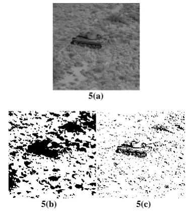
Here three input images and their output images are shown in Fig. 3 – Fig. 5. All the images are gray level images of size 256 × 256. The Lena image, the binarized image using k-means and the binarized image by the proposed method are shown in Fig. 3(a), 3(b) and 3(c) respectively. The Horse image, the binarized image using k-means and the binarized image by the proposed method are shown in Fig. 4(a), 4(b) and 4(c) respectively. The Tank image, the binarized image using k-means and the binarized image by the proposed method are shown in Fig. 5(a), 5(b) and 5(c) respectively. From the figures (Fig. 3 – Fig. 5) it is observed that the outputs of the proposed method are better than the outputs of the k-means method.

3(a)

3(b) 3(c)

Figure 3(a): Lena image; 3(b): Binarized image using K-Means; 3(c): Binarized image using proposed method

4(a)

4(b) 4(c)

Figure 4(a): Horse image; 4(b): Binarized image using K-Means; 4(c): Binarized image using proposed method

5(a)

5(b) 5(c)

Figure 5(a): Tank image; 5(b): Binarized image using K-Means; 5(c): Binarized image using proposed method

Figure 6(a): Lena histogram

Figure 6(b): Horse histogram

Figure 6(c): Tank histogram

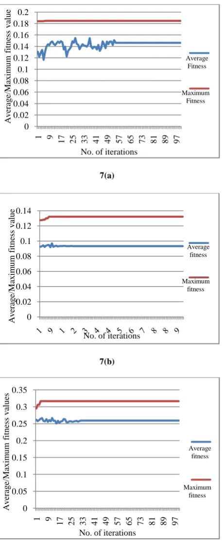
The graphs of the average and maximum fitness values are also shown in Fig. 7(a), 7(b) and 7(c) respectively. These are the plots of each of the images which when applied to the genetic algorithm give these values. As we can see the plots become stable after some iteration.

7(a)

7(b)

7(c)

Figure 7: (a): Lena average / maximum plot, (b): Horse average / maximum plot, (c): Tank average / maximum

plot 0 100 200 300 400 500 600 700

0 _{16 32 48 64 80 96}

112 128 144 160 176 192 208 224 240

F re q u en cy o f p ix els Intensity values Histogram-Lena 0 200 400 600 800 1000 1200 1400 1600 1800 0

16 32 48 64 80 96 _{112 128 144 160 176 192 208 224 240}

F re q u en cy o f p ix els Intensity Values Histogram-horse 0 200 400 600 800 1000 1200 1400 1600

0 _{16 32 48 64 80 96}

112 128 144 160 176 192 208 224 240

F re q u en cy o f p ix els Intensity Values Histogram-Tank 0 0.02 0.04 0.06 0.08 0.1 0.12 0.14 0.16 0.18 0.2 1 9

17 25 33 41 49 57 65 73 81 89 97

A v era g e/M ax im u m f it n ess v alu e

No. of iterations

Average Fitness Maximum Fitness 0 0.02 0.04 0.06 0.08 0.1 0.12 0.14 A v era g e/M ax im u m f it n ess v alu e

No. of iterations

Average fitness Maximum fitness 0 0.05 0.1 0.15 0.2 0.25 0.3 0.35 1 9

17 25 33 41 49 57 65 73 81 89 97

A v era g e/M ax im u m f it n ess v alu es

No. of iterations

Average fitness

5.

CONCLUSIONS

This paper presents a simple but effective method for image binarization. The effectiveness of the proposed method has been proven by the experimental results on images from a standard image database. Testing the noise immunity of the proposed method and further tuning of the parameters used can lead to better results in future.

Also, there is a future scope of experimenting with document images, colored images, even in the analysis of medical images and change detection in remote-sensing images, etc. Change Detection, in particular, is a very important application that uses the concept of Image Binarization. It can be used for variety of applications, such as the quantification of re-vegetation activities in disturbed areas; monitoring of facilities, movement of oil spills (land and sea), pipeline encroachment, and changes in ice/snow extent.

6.

REFERENCES

[1] Schwefel, H.P. and Rudolph, G. 1995. Contemporary evolution strategies. Advances in artificial life, 893 – 907.

[2] Paulinas, M. and Ušinskas, A. 2007. Survey of genetic algorithms applications for image enhancement and segmentation, Information technology and control, 36(3), 278-284.

[3] Mitchell, M. 1996. An introduction to genetic algorithms. The MIT Press, 208.

[4] Holland, J.H. 1975. Adaptation in Natural and Artificial Systems, MIT Press.

[5] Faber, V. 1994. Clustering and the Continuous k-Means Algorithm. Los Alamos Science, 138-144.

[6] Ostu, N. 1978. A thresholding selection method from gray-level histogram, IEEE Trans. Systems Man Cybernet. SMC-8, 62-66.

[7] Sahoo, P.K., Soltani, S. and Wong, A.K.C. 1988. A survey of thresholding technique, Comput. Vision Graphics Image Process. 41, 233-260.

[8] Kapur, J.N., Sahoo, P.K. and Wong, A.K.C. 1985. A new method for gray-level picture thresholding using the entropy of the histogram, Computer Vision Graphics Image Process. 29, 273-285.

[9] Lee, S.U., Chung, S.Y. and Park, R.H. 1990. A comparative performance study of several global thresholding techniques for segmentation, CVGIP 52, 171-190.

[10]Boukharouba, S., Rebordao, J.M. and Wendel, P.L. 1985. An amplitude segmentation method based on the distribution function of an image, Computer Vision Graphics Image Process. 29, 47-59.

[11]Wang, S. and Haralick, R.M. 1984. Automatic multithreshold selection, Computer Vision Graphics Image Process. 25, 46-67.

[12]Kohler, R. 1981. A segmentation system based on thresholding, Computer Graphics Image Process. 15, 319-338.

[13]Papamarkos, N. and Gatos, B. 1994. A new approach for multilevel threshold selection, CVGIP: Graphical Models Image Process. 56(5), 357-370.

[14]Niblack, W. 1986. An Introduction to Digital Image Processing. Prentice Hall, Eaglewood Cliffs 115–116. [15]Sauvola, J. and Pietikainen, M. 2000. Adaptive document

image binarization. Pattern Recogn. 33(2), 225–236. [16]Shaikh, S.H., Maiti, A. K. and Chaki, N. 2011. A New

Image Binarization Method using Iterative Partitioning, Springer Journal on Machine Vision and Applications; 281-286.