MODLE REDUCTION IN BIOMECHANICS
Yan Feng
A dissertation submitted to the faculty of the University of North Carolina at Chapel Hill in partial fulfillment of the requirements for the degree of Doctor of Philosophy in the
Department of Mathematics.
Chapel Hill 2017
©2017 Yan Feng
ABSTRACT
Yan Feng: Model Reduction in Biomechanics (Under the direction of Sorin Mitran)
from experimental results. However, in real biological world, these homogeneous and isotropic assumptions are usually invalidate. Thus, instead of using hypothesized model, a specific continuum model at mesoscopic scale can be introduced based upon data reduction of the results from molecular simulations at atomistic level. Once a continuum model is established, it can provide details on the distribution of stresses and strains induced within the biomolecular system which is useful in determining the distribution and transmission of these forces to the cytoskeletal and sub-cellular components, and help us gain a better understanding in cell mechanics.
To my brilliant and outrageously loving and supportive husband, Hongchuan Wei, my always encouraging, ever faithful parents, Fuzeng Feng and Pei Yan, and to my many friends and church
ACKNOWLEDGEMENTS
Firstly, I would like to express my special appreciation and thanks to my advisor Sorin Mitran for the continuous support of my Ph.D study and related research during these past five years. I appreciate all his contributions of time, ideas, and funding to make my Ph.D. experience productive and stimulating. He has provided his scientific advice and knowledge and many insightful discussions and suggestions. I could not have imagined having a better advisor and mentor for my Ph.D study. I am also thankful for the excellent example he has provided as a successful mathematician and professor.
Besides my advisor, the members of the Cell Mechanics group have contributed immensely to my Ph.D study at UNC. The group has been a source of friendships as well as good advice and collaboration. I am especially grateful for the fun group of original Cell Mechanics group members: Michael Falvo, Timothy O?Brien and Richard Superfine, for multiple discussions on mechanics of the microtubule and cells and relevant experimental observations.
I would also like to thank the members of my PhD committee, Professors Michael Falvo, Richard Superfine, Nancy Rodriguez, and Katie Newhall for serving as my committee members and letting my defense be an encouraging and enjoyable moment, for their insightful comments and encouragement to widen my research from various perspectives.
TABLE OF CONTENTS
LIST OF TABLES . . . x
LIST OF FIGURES . . . xi
LIST OF ABBREVIATIONS . . . xvi
1 INTRODUCTION . . . 1
1.1 The mechanics of the cell . . . 1
1.2 Cytoskeleton system . . . 2
1.3 Cell mechanics and human disease . . . 6
1.4 Techniques in cell mechanics . . . 6
1.5 Challenge in cell Mechanics . . . 9
2 REDUCED MODELS FOR BIOMOLECULAR SYSTEM . . . 11
2.1 Introduction . . . 11
2.2 Multiscale challenges in biomolecular system . . . 12
2.3 Atomic coarse-grained models . . . 14
2.3.1 Level of resolution . . . 15
2.3.1.1 Clustering analysis . . . 15
2.3.1.2 Clustering analysis on tubulin dimer . . . 16
2.3.2 Force field . . . 18
2.3.2.1 Elastic network models . . . 19
2.3.2.2 Self-organized polymer model . . . 21
2.4 Model Reduction via Principal Orthogonal Decomposition . . . 22
2.5.1 Model reduction via principal orthogonal decomposition . . . 24
3 MODEL REDUCTION ON 3D STATIC LINEAR ELASTICITY PROBLEM . . . 26
3.1 Introduction . . . 26
3.2 The System of elasticity . . . 27
3.3 Finte element method . . . 29
3.4 Model reduction on 3D static linear elasticity problem. . . 32
3.4.1 Finite element method in solving 3D static linear elasticity problem . . . 32
3.4.2 Euler-Bernoulli beam theory. . . 35
3.4.3 Model reduction on 3D static linear elasticity problem . . . 39
3.4.3.1 POD modes of 3D linear system of elasticity . . . 39
3.4.3.2 2D POD beam element . . . 43
3.4.3.3 Comparison of 2D Euler-Bernoulli beam element and POD beam element . . . 46
4 MODEL REDUCTION ON MICROTUBULE MECHANICS . . . 47
4.1 Introduction . . . 47
4.2 Cell mechanics . . . 48
4.3 Microtubule structure . . . 49
4.4 Mechanics of Microtubule . . . 50
4.4.1 Experimental measurement . . . 51
4.4.2 Computational estimations of bulk moduli . . . 51
4.5 Atomic CG-SOP model of microtubule . . . 54
4.6 Reduced normal mode analysis. . . 59
4.7 Data-driven beam model of microtubule . . . 62
4.8 Result . . . 65
4.8.1 Atomistic microtubule deformation data. . . 65
4.8.2 Reduced atomistic normal modes . . . 68
4.8.4 Cantilever structure with tip load . . . 75
4.8.5 Vibrational modes of a microtubule . . . 78
5 Applications . . . 82
5.1 Introduction . . . 82
5.1.1 Microtubule functions . . . 82
5.1.2 Cilia and flagella . . . 83
5.2 Modeling of microtubule doublet . . . 84
5.2.1 Cantilever structure with distributed force . . . 86
5.3 Modeling of axoneme . . . 86
5.3.1 Cantilever structure with distributed force . . . 88
5.4 Modeling of mitosis spindle pole separation . . . 88
5.5 Conclusions . . . 90
LIST OF TABLES
3.1 Comparison of 2D Euler-Bernoulli beam element and POD beam element. . . 46
4.1 Microtubule stiffness measured by AFM and other experimental techniques . . . 52 4.2 Microtubule stiffness measured by computational modeling and simulations . . . 53 4.3 Comparison of free vibration frequencies of an Euler-Bernoulli model of a
LIST OF FIGURES
1.1 The components of the cytoskeleton (Johnson, George B. The Living World). . . 3
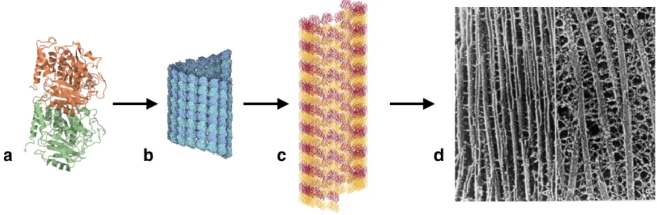
2.1 A visual representation of the multiscale challenge for understanding in biological systems. (a) an atomistic representation of a tubulin dimer (PDB, 1tub); (b) a microtubule fragment, made up of many tubulin dimers (PDB, 3j2u ); (c) a coarse-grained representation of a microtubule frag-ment, which reduce the computational cost for simulation; (d) a meso-scopic cytoskeleton network made up of many individual microtubules. (http://w3.impa.br/ jair/summary1.html) . . . 13
2.2 (a) Diagrams of theαβ-tubulin dimer. Coordinates forαβ-tubulin are taken from the Protein Data Bank, code1TUB. (b) Coarse-grained structure after replacing the main chain with theCα atom. . . 15
2.3 Clustering analysis on tubulin dimer. . . 17
2.4 (a) Diagrams of the αβ-tubulin dimer. Coordinates for αβ-tubulin are taken from the Protein Data Bank, code1TUB, and the tubulin dimer is represented by a virtual backbone. (b) Coarse-grained model of tubulin dimer by theCα atom representation. (c) The elastic network model of tubulin dimer, and each interaction sites are identified by theCα atoms which connected by the springs when the distance with in a cutoff distance. . . 19
2.5 Residue pair: a virtual backbone between two interaction sites (Cαatoms). Within a cutoff distanceRcaround the central residuei, the residue pairs are subject to an interacting force. The residue pairs are subject to a harmonic force provided that they are within a cutoff distance range of1.2nm around the residuei. Dotted lines designate the residues interacting with that residue. . . 20
3.1 Components of stress in three dimensions. . . 27
3.2 Finite element discretization and extraction of generic element. . . 30
3.3 FreeFem++implementation of the finite element method in 3D static linear elasticity problem in beam shows the initial mesh and distorted mesh after bending, respectively. . . 33
3.4 Initial mesh(light) and distorted mesh after stretching (dark), respectively. . . 34
3.5 Initial mesh(light) and distorted mesh after shearing (dark), respectively. . . 34
3.7 A single 2D Euler-Bernoulli beam element of two nodes, with three degrees of freedom at each node, two translationsu,v and one rotationθ, is used
to represent the 3D linear system of elasticity. . . 35 3.8 A single 2D Euler-Bernoulli beam element of two nodes, with three degrees
of freedom at each node, two translationsu,v and one rotationθ, is used
to represent the 3D linear system of elasticity. . . 37 3.9 FreeFem++implementation of stretching/compression simulation on 3D
linear system of elasticity. Initial mesh (orange, dark) and distorted mesh
(yellow, light), respectively. . . 39 3.10 FreeFem++implementation of shearing simulation on 3D linear system
of elasticity. Initial mesh(orange, dark) and distorted mesh after shearing
(yellow, light), respectively. . . 39 3.11 FreeFem++implementation of bending simulation on 3D linear system
of elasticity. Initial mesh (orange, dark) and distorted mesh after bending
(yellow, light), respectively. . . 40 3.12 The log plot of the importance of eigenvalueλi , Pmλi
i=1λi, of correlation
matrixC. The first three modes are the most dominant modes. . . 41 3.13 FreeFem++implementation of bending simulation on 3D linear system
of elasticity. Initial mesh (orange, dark) and distorted mesh after bending
(yellow, light), respectively. . . 42 3.14 POD modes. Initial mesh (orange, light) and distorted mesh (yellow, dark),
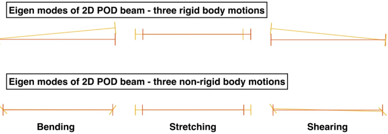
respectively. . . 43 3.15 Eigen modes of 2D POD beam - three rigid body motions and three
non-rigid body motions. Initial mesh (orange, dark) and distorted mesh (yellow,
light), respectively. . . 44
3.16 FreeFem++implementation of (a) stretching/compression simulations, (b) shearing simulations, and (c) bending simulations on 3D linear system of
elasticity. Initial mesh(orange, dark) and distorted mesh (yellow, light), respectively. 45 3.17 Beam element is fixed at one end and subjected to a point loadFextat its
free end. Initial configuration (orange, dark) and distorted configuration
(yellow, light), respectively. . . 46
4.1 (a) Motile cilia on airway epithelial cells. (b) Electron micrograph of cilium showing longitudinal and transverse sections. (Micrographs are copyright Gwen C. Childs,http://cytochemistry.net/cell-biology/
4.2 The microtubule lattice obtained by docking the crystal structure of the tubulin protofilament into a reconstruction of the microtubule. Sequences ofα-tubulin (light) andβ-tubulin (dark) repeat along each protofilament in
a longitudinal direction. . . 50 4.3 Coarse-graining procedure for constructing a SOP model of aαβ-tubulin
dimer. The amino acid residues are replaced by single interaction centers (spherical beads) with the coordinates of theCα-atoms (represented by the black circles). Within a cutoff distanceRcaround the central residuei, the
residue pairs are subject to an interacting force. . . 55 4.4 (a) Different types of native contact between CG sites in SOP model and
associating values ofεh. . . 57 4.5 Reduction in computational complexity from full atom model to CG-SOP
model of microtubule fragment. . . 58 4.6 CG-SOP model subjects to different types of external forces Fext, that
principally induce (a) stretching / compression, (b) shearing, (c) bending,
(d) twist. . . 58 4.7 When the whole microtubule is divided into small segment/fragment, the
overall behavior of the microtubule is determined by the translation and rotation of each segment. Thus, the overall behavior of the microtubule is determined by the translations and rotations of each fragment which can
be evaluated by the cross-sections at two ends. . . 63 4.8 MTDDBM: microtubule-beam element is used to represent microtubule fragment. . . 64 4.9 The normal modes of MTDDBMVb are obtained by selecting
dominant-modes from the reduced normal mode analysis of the atomistic CG-SOP
model. . . 64 4.10 SOP simulations, schematic diagrams of deformation and force-
displace-ment plots. . . 66 4.11 Force-displacement plots: (Left) Stretching atomistic CG-SOP simulations
of microtubule fragment. The arrows indicate the direction of force. Total axial displacement δz along z-axis versus force F is plotted. (Middle) Bending atomistic CG-SOP simulations of microtubule fragment. The arrows indicate the moment. Total angular displacementδθy along y-axis versus momentM is plotted. (Right)Twist atomistic CG-SOP simulations of microtubule fragment. The arrows indicate the torque. Total angular
4.12 Bending deformation response of a protofilament. Each dot corresponds to the magnitude of a bending moment applied at extremal tubulin dimers at the angle in the xy indicated at end of locus of point sequence. The resulting deformation angles are shown as abscissa and ordinate values. In-plane bending would be represented as radial locii, but the protofilament
exhibits marked deviation from in-plane bending. . . 69 4.13 Normal modes of72.54nm long microtubule fragment: three characteristic
non-rigid body motions, (a) compression, (b) bending, and (c) twist. . . 70 4.14 Visualization of coefficient matrices for EEBM and MTDDBM. . . 76 4.15 (a) A cantilever structure constructed by microtubule-beam element is
loaded by a point loadP at its free end. (b) Displacement versus load plot. . . 76 4.16 (a) Cantilever structure constructed by microtubule-beam element (dark)
and 3D linear elastic beam element (light) are loaded by a point loadP at its free end alongx-direction. (b) Displacement along alongx-direction
versus load plot. (c) Displacement along alongy-direction versus load plot. . . 78 4.17 (a) Twist simulations. The arrows indicate the moment. (b) Total angular
displacement versus Torque plot. . . 79 4.18 (Top row) Three-dimensional view of six lowest frequency modes of free
vibration of anLM T =6720 nm microtubule fragment as determined from MTTDDBM model. (Bottom row) Top view showing coupling of bending
vibrations in orthogonal planes. . . 80
5.1 a. SEM micrograph of the cilia projecting from respiratory epithelium in
the lungs. b. SEM image of desulfovibrio species. . . 83 5.2 (a) Projection image of the final doublet density map along the longitudinal
axis. (b) Interpretation of the 3D density map. Axial view, seen form the proximal end, of the tomographic reconstruction that was filtered to enhance 16-nm spacings, viewed as an isosurface (yellow). The pseudo-atomic model (backbone only) fitted to the doublet density is shown in blue
with labels assigned to the protofilaments. (Sui and Downing, 2006) . . . 84 5.3 (a) Backbone representation of microtubule doublet. The atom coordinates
are available at protein data bank (PDB) with accession number 3JAO. (b) Cross-section of microtubule doublet. A-tubule and B-tubule are fitting
into two ellipses, and the dots are the center of mass of the protofilaments. . . 85 5.4 A cantilever structure of microtubule doublet constructed by MTDDBM
element is loaded by a distributed force. The arrow indicates the direction
5.5 a. Electron micrograph of a cross-section of a Chlamydomonas flagellum (Molecular Cell Biology, nature review). b. Diagram of structure of ciliary
and flagellar axonemes (Molecular Cell Biology, 4th edition). . . 88 5.6 A cantilever structure of cilia constructed by MTDDBM element is loaded
by a distributed force, and force-displacement plot of cilia model. . . 89 5.7 (a) Mitotic spindle component model. Two microtubules and molecular
sliding motors. (b) Typical result showing differences in deformation behavior between Euler-Bernoulli and MTDDBM models. (c) Spindle
elongation-sliding force plot for the Euler-Bernoulli and MTDDBM models. . . 92 5.8 (a-c)Two overlapping microtubules modeled by microtubule-beam element
and 3D elastic beam element are loaded by a sliding forceFsat the overlap-ping region different boundary conditions: (a) fixed rotation aroundz-axis, (b) the angle of rotation limited by a allowed torque, and (c) free rotation
LIST OF ABBREVIATIONS
MT Microtubule
CG Coarse-Graining
MD Molecular Dynamics
RTB Rotation-Translation of Blocks ENM Elastic Network Models SOP Self-Organized Polymer
POD Proper Orthogonal Decomposition
NMA Normal Mode Analysis
FEM Finite Element Method
DOF Degrees Of Freedom
PDB Protein Data Bank
DDBM Data-Driven Beam Model
CHAPTER 1: INTRODUCTION
1.1 The mechanics of the cell
The cell is the smallest and most basic structural, functional, and biological unit of life. Cells consist of cytoplasm enveloped by a membrane, which takes up most of the cells’ volume and contains many functional biomolecules such as cytoskeleton, organelles and nucleic acids (Hardin et al., 2015). Animals, plants and fungi are eukaryotes, namely cells that contain a nucleus, as distinguished to prokaryotic cells. The eukaryotic cell relies on the cytoskeletal system to maintain or change the cell shape during movement, to resist mechanical deformation, to transport intracellular cargo, and to stabilize entire tissues by associating with extracellular connective tissue and other cells.
Tremendous efforts have been made by the biologist trying to elucidate the structure and function of the cells, how they interact with other cells and extracellular environment physiologically and biologically, as the basic topic in cell biology. In this field, the study of the cell at the molecular level mainly focus on chemistry, the laws governing the interaction between molecules that results in the formation and breakage of chemical bounds, and physics, the laws governing molecular structure and properties. Despite the progress on the study of individual molecules, we still seek better understanding of how these molecules interconnect dynamically and adaptively to create coupled regulatory networks. Recently, the emergence of biomechanics, which integrates mechanics, molecular biology, biophysics, biochemistry and biomolecular engineering, unfolds the role of the mechanical force during many fundamental cellular processes.
describing non-Newtonian viscosity. In the 1920s microscopic magnetic particles were manipu-lated within live cells to obtain quantitative measurements of elastic and viscous parameters by microrheology. In part, the focus on cell mechanics has been motivated by efforts to define how cells perform mechanical work as they move; however, recently, increased interest in cell mechanics has been generated by demonstrations that the mechanical features of the extracellular environment and application of forces to cells trigger cellular responses that are essential for many aspects of cell structure and function.
In contrast to the level of understanding of how specific chemicals trigger and transduce signals within cells, studies of how cells sense force and how they respond to different levels, durations, and directions of force are much less common, but have recently attracted increasing attention from biologists and bioengineers. Defining specific structures and mechanisms by which forces, both external and internally generated, are sensed by cells and how this stimulus leads to specific responses is likely to help explain the complex functions of cells and to design better materials for cell and tissue engineering and other applications in vivo.
1.2 Cytoskeleton system
Figure 1.1: The components of the cytoskeleton (Johnson, George B. The Living World).
types of polymers comprising the cytoskeleton as shown in Fig (1.1): actin filaments, microtubules and a group of polymers known collectively as intermediate filaments. These cytoskeletal structures are multifunctional and well-arranged into a regulatory network, which is able to respond to the external applied force and resists the deformation to maintain the integrity of the cell in shape. Meanwhile, the actin filaments and microtubules undergo conformational changes, polymerization and depolymerization, at the two ends of the polymers in response to GTP hydrolysis, a property known as dynamic instability. It has been found that many cellular processes are powered by this property of cytoskeleton, because the polymerization and depolymerization of microtubule and action filaments generate directed force, together with molecular motors, that drive the movement of the cellular structures. For example, during mitosis, as the growth and shrinkage of the microtubules inside mitotic spindle, the chromosomes are pushed or pulled around to regulate the process of cell division. Different structures of these three polymers define their distinctions in the mechanical stiffness, the dynamics of the self-assembly process, the polarity and the kind of associated molecular motors, resulting in different architectures and functions to the networks they form.
decades help to furnish microtubule mechanical properties by the many experimental techniques, such as optical tweezers, thermal fluctuation, buckling force measures method and hydrodynamic flow. However, despite the imaging techniques allow the visualization of a single protein and the applied external forces can be measured by high precision mechanical probes, the determination of the mechanical properties of the microtubule was not an easy task due to its nonlinear, history dependent nature of stress-strain relationships. On the measurement of the flexural rigidity of microtubules, it is typical to introduce a Euler-Bernoulli beam model to interpret the measures resulting in values of Young’s modules between Mpa to Gpa. All of the methods mentioned assumed that the microtubule is a homogeneous and isotropic slender elastic rod. The validity of this assumption if open to question, since microtubules are highly anisotropic structure.
filaments are the smallest cytoskeletal filaments, with a diameter of 7nm, but widely distributed throughout the cell and contributing to the regulation of many cellular activities. They are the primary cytoskeletal component to drive cell motility by organizing into a highly branched fila-mentous network to support the leading edge of moving cell. During cell division, the disassembly of the actin-based motile structures generate the forces that causes the cell to stop moving and become more rounded. Unlike microtubules, actin filaments do not switch between discrete states of polymerization and depolymerization. During polymerization, G-actin aggregates into short, unstable oligomers, which elongate steadily into a filament by addition of actin monomers to both of its ends until the steady-state phases reached. Assembly of actin filaments from their monomeric subunits and the formation of actin-filament bundles and networks suffice to change the shape of the cell and produce a protrusion the for cell migration.
Another important property of both microtubule and actin filaments is polarity due to the asymmetrical structure and uniformly stacked orientation of their subunits at the molecular level. As a result of this structural polarity, both types of polymer function as suitable tracks for molecular motors that move preferentially in one direction. For microtubules, the motors are members of the dynein or kinesin families, whereas for actin filaments, they are members of the large family of myosin proteins. These molecular motors have essential roles in organizing the microtubule and actin cytoskeletons. Microtubule-associated motors are crucial for the assembly of the microtubule array, in interphase, and the mitotic spindle. These motors also carry cargo between intracellular compartments along microtubule tracks.
1.3 Cell mechanics and human disease
A rapidly growing body of science indicates that mechanical phenomena are critical to the proper functioning of several basic cell processes and that mechanical loads can serve as extracellular signals that regulate cell function. Further, disruptions in mechanical sensing and/or function have been implicated in several diseases considered major health risks, such as osteoporosis, atherosclerosis, and cancer. At its most basic level, hearing is a process of transduction. A physical signal in the form of sound (pressure) waves is converted into electrical impulses along a nerve. Mechanotransduction occurs in the ear via a specialized cell called the inner ear hair cell. When sound is transmitted to the inner ear, the vibrations cause the cilia to deflect, which in turn stretches the actin filaments. The kinetics of signaling proteins inside the cell are altered by the change of calcium concentration, and a cascade of biochemical events is initiated that eventually leads to a depolarization of the cell and a nerve impulse. Mechanics is very important in this process. The cilia need to have the right mechanical characteristics to stand upright, but remain flexible enough that they can be deflected by sound waves. The actin tip kinks need to be strong enough to open the channel and to have the appropriate polymer mechanics behavior so that they are stretched by cilium deflection, but are not affected by thermal noise.
1.4 Techniques in cell mechanics
experimental challenges in molecular biomechanics involve the need to study molecular complexes in conditions closer to their in vivo environment
Progress in cell biology has been facilitated and complemented by the increasing capability of computer power to fulfill the multi-scale simulations with nearly real timescale. Computational techniques, including molecular dynamics (MD), Monte Carlo methods, and Brownian dynamics calculations, have the potential to complement the single-molecule experimental investigations, and provide insight into the underlying mechanisms with atomic resolution. In addition, several computational tools have been developed for molecular biomechanics studies such as steered molec-ular dynamics(SMD), the umbrella sampling technique and normal mode analysis. Together these computational techniques are used to determine mechanical and physical properties of molecules that account for their functional roles. Computational techniques have been used to study a variety of issues in molecular biomechanics. One of the most important applications of computational molecular biomechanics is the study of mechanotransduction, the process by which cells transduce mechanical signal into biological processes.
computational demands. The timescale is severely limits the applicability of MD simulation, since the available computing power prevents simulations over times longer than microseconds while most of the biological processes in a living cell occur with a timescale longer than a few milliseconds.
In the real biological context of the cellular cytoskeleton, multiple scales and spatiotemporal coupling occur: an atomistic- scale dimension is generally coupled to one or more mesoscale dimensions, and this in turn is coupled to the near-continuum scale. In this case, the explicit motions of every atom is the system contain more information than is needed or even desirable to describe the essential features of the problem. In this context, coarse-grained is ideal representation which reduce the number of degrees of freedom of the system and bridge the atomistic and mesoscopic scales to make true multi-scale simulations feasible. Coarse-grained therefore provides a highly significant advance in the field of biomolecular modeling and simulation. However, several substantial challenges emerge when the coarse-grained approach is employed instead of atomistic MD. One of the challenges involves the establishment of a proper formal connection between the behavior of the coarse-grained representation of the system and the underlying all-atom (full atomic resolution) model. Additional challenges involve the degree of believable predictive power of the coarse-grained models and their transferability between dissimilar systems. These challenges are a direct result of the reduction in the resolution of the system by the coarse-grained procedure and the resulting risk of losing certain key information.
1.5 Challenge in cell Mechanics
Comprehensive mechanical analysis of a cell is extremely complex. The mechanical prop-erties of the cell are essential to force responses because they determine the extent of deformation of the region of the cell where the force is applied, and therefore the range of molecular deformations that can be triggered. Lots of efforts have been made trying to answer the basic question in cell mechanics: how to determine or what determines stiffness and other constitutive physical properties of the cell? Estimates of cellular stiffness derived from different types of micro-rheological methods cover a wide range depending on the methods used, the type and extent of deformation, and the time that the deformation is applied. There are one-dimensional linear elements in the cytoskeleton and two-dimensional solids and enormous potential for pressure effects and fluid-solid interaction. Indeed, the overall cell is part-solid, part-liquid, something we call viscoelastic.
The values of elastic moduli calculated from force-deformation studies of cells are inher-ently difficult to interpret even when the experimental results are highly reproducible and well controlled. Among the factors that complicate the analysis are the facts that the structure of the cell interior is not homogeneous. For example, the flexural rigidity of microtubules, based upon an assumed Euler-Bernoulli beam model, has been estimated using optical tweezers, thermal fluctua-tions, buckling force measurements, and hydrodynamic flow interactions. Published values for the resulting Young’s modulusE vary between 3.1±0.9 MPa and 1.4 GPa, a three-order of magnitude discrepancy. Published values for the shear modulus also exhibit marked discrepancies ranging from 1.4 Pa to 1.4 MPa. Clearly, more than variability due to experimental technique, the possibility of incorrect assumptions on the mechanical behavior of a microtubule has to be considered. Therefore, the elastic modulus calculated from subcellular deformations is model dependent.
CHAPTER 2: REDUCED MODELS FOR BIOMOLECULAR SYSTEM
2.1 Introduction
2.2 Multiscale challenges in biomolecular system
Advances in molecular modeling and simulation, especially the all atom simulations of single molecule, have significantly contributed to the knowledge of the behavior of individual biological molecule. During the last two decades, single-molecule experiments have developed into a mature stage, and provided rich molecular information for the studies of complex biological systems and processes. Computational simulations on the single molecule are used to collaborate and complement the experimental results, for example, in the field of biomechanics, modeling of single molecule under mechanical manipulation and control helps to verify the experimental measurement of molecular forces and the molecular structural and functional responses. The most successful and widely used computational technique for the studies on the single molecule is molecular dynamics (MD) simulation, which is atomic model routinely carrying out for the systems having tens of thousands of atoms in length scale and lasting microseconds even millisecond in time scale. However, MD simulation is not feasible to investigate large molecular system in the real biological context based on the state-of-the-art computer power. For the exploration of mesoscopic phenomena of real biomolecular systems, the size of the system increases to million of atoms, then time scale has to be compromised to tens or hundreds of nanoseconds in MD simulation while most of the biological processes in a live cell longer than a few milliseconds.
Figure 2.1: A visual representation of the multiscale challenge for understanding in biological systems. (a) an atomistic representation of a tubulin dimer (PDB, 1tub); (b) a microtubule fragment, made up of many tubulin dimers (PDB, 3j2u ); (c) a coarse-grained representation of a microtubule fragment, which reduce the computational cost for simulation; (d) a mesoscopic cytoskeleton network made up of many individual microtubules. (http://w3.impa.br/ jair/summary1.html)
greatly simplified and much more computationally efficient CG microtubule representation (Figure 2.1 c), which might, e.g., be used to model the mesoscopic cytoskeleton network depicted at the near-continuum scales (Figure 2.1 d ).
Also, Fig (2.1) depicts some of the multiple scales that exist in the particular example of the cellular cytoskeleton, beginning with the basic tubulin dimer ”building block” (Figure 2.1 a). With all such biomolecular systems, an atomistic-scale dimension is generally coupled to one or more mesoscale dimensions, and this in turn is coupled to the near-continuum scale, in this case the cytoskeleton network (Figure 2.1 d). It means that the details resulting from atomistic-scale (molecular) domains are ultimately crucial in determining the collective properties of the highest scales, but when the overall behavior of the biomolecular system at the near-continuum scale is investigated, the explicit motion of each atom at the atomistic-scale is no longer necessary or even desirable to describe the essential features of the problem.
length scale dynamics that are critical to many biological processes. In such case, coarse-graining has become a rapidly expanding methodology in the field of biomolecular simulation to largely reduce the computational cost. A greatly simplified and much more computationally efficient CG representation can reveal how molecular-scale changes and transformations propagate upward in scale to define the function of biological structures.
2.3 Atomic coarse-grained models
In fact, the all-atom simulation, such as MD simulation mentioned above, can be considered as coarse graining modeling which averages out the degrees of freedom of quantum mechanical system to enable the modeling and simulation at atomic level. Similarly, the atomic CG model aver-ages out the atomic degrees of freedom by clustering groups of atoms into new coarse-grained (CG) sites, or called ”pseudoatoms”, and provides insight into the overall behavior of the biomolecular system. The reduction in the total number of degrees of freedom of the system accomplished by atomic CG model allows for a significant increase over both the spatial and temporal limitations of all-atom models.
Since atomic CG models are neglecting some atomic degrees of freedom, both structural information and interactions, they can be considered as lower resolution models to capture certain key feature of the system in order to investigate the mesoscopic phenomena of interest. For the exploration of large-scale simulation of biomolecular systems, atomic CG models have gained a lot of popularity lately due to their advantages, in both length and time scale, over the all-atom models: atomic CG models can handle the system with millions of CG sites, and they allow for the simulation of slow processes which require time scales in the microsecond to millisecond range.
2.3.1 Level of resolution
The level of model resolution, which can be atomic, mesoscopic even continuum, deter-mines the reduction in the total number of degrees of freedom of the system and the applicability of this reduced model. Since it has been found that there is no intrinsically optimal number of CG sites for a given system, the level of the resolution is chosen based on the size of the system investigated and the certain feature of this biomolecular system addressed. In some models, all
a
α-Tubulin
β -Tubulin
α-Tubulin
β -Tubulin
b
α-Tubulin
β -Tubulin
Figure 2.2: (a) Diagrams of theαβ-tubulin dimer. Coordinates forαβ-tubulin are taken from the Protein Data Bank, code1TUB. (b) Coarse-grained structure after replacing the main chain with the Cαatom.
main chain atoms are treated in an explicit way while in others single united atoms replace the side groups. Sometimes, the main chain could be replaced by theCα atom, which is the first carbon atom that attaches to a functional group , and the side chains partitioned into several interacting units as shown in Fig (2.4). The mapping from group of atoms to a single CG site at the new CG location is specified as well, and one example of such mapping function is the center of mass of a group of atoms.
2.3.1.1 Clustering analysis
of certain group of atoms can also be detected by certain algorithms, such as hierarchical clustering analysis on the correlation matricesC, which describe the atomic pairwise dynamics of the system (Keskin et al., 2002).
The orientational cross-correlations between the fluctuations of theCαatoms are found by normalizing the cross-correlations according to
Cij =
<∆Ri·∆Rj >
(<∆Ri·∆Ri ><∆Rj·∆Rj >) 1 2
, (2.1)
where∆Ri represents the fluctuation of residuei. <∆Ri·∆Rj >is calculated from< ∆Ri· ∆Rj >=kTtrace[H−ij1], andHis the Hessian matrix readily calculated by taking second derivative of potential with respect to the position of residues. The positive and negative limits of correlation matricesCare 1and −1, which correspond to pairs of residues exhibiting fully correlated and fully anticorrelated motions, respectively. Correlations between residue fluctuations describe those parts of the structure that move collectively, as a unified group, and how these regions move with respect to one another. Based on the correlation matrix, clustering analysis provides a method for clustering the Cα atoms into the optimum number of clusters, which finds the similarity or dissimilarity between every pair of Cα atoms to identify the collective motions of biomolecular system.
2.3.1.2 Clustering analysis on tubulin dimer
K means clustering: k = 2, silhouette = 0.77
K means clustering: k =4, silhouette = 0.50
K means clustering: k=6, silhouette = 0.49
Silhouette value
Silhouette value
Silhouette value
Cluster
Cluster
Cluster
k = 8 k = 10 k = 12
0 5 10 15 20 25 30 35 Number of clusters
0.8
0.6 0.7
0.5
Silhouette value
0.4
Clustering Method: kmeans Clustering Method: linkage
Figure 2.3: Clustering analysis on tubulin dimer.
to describe biomolecular systems. The application of this coarse-graining technique is relatively straightforward, and should be widely applicable to other macro- molecular systems and larger macromolecular complex.
When the cluster numberk = 6, the silhouette value is about 0.5, and each monomer is further partitioned into three clusters. These three clusters of α- and β- monomer obtained by clustering analysis is reasonably consistent with its functional domain found by Nogales: nucleotide-binding domain having a typical Rossmann fold, an intermediate domain containing the Taxol-binding site, and the carboxy-terminal domain, which constitutes the binding surface for MT-associated motor proteins. These three functional domains are also called: N-terminal domain, intermediate domain and C-terminal domain, respectively. By the inspection of the correlation map, each tubulin monomer shows symmetrical opposite direction movements with respect to the dimer interface, while N- and C- terminal domain exhibit some tendency to move in the same direction whereas the intermediate domain of the molecule under- goes mostly opposite direction motions. Grouping together the residues with the most similar correlated patterns could provide significant insight into the global motion of the tubulin dimer. For example, RTB method can be implemented by dividing the whole system into n rigid blocks, and each block is made of a certain number of residues. By the correlation mapping, three rigid domains were identified in each tubulin monomer which is corresponding to the three functional domains. Deriu et al. (Deriu et al., 2010) simulated coarse-grained models of entire microtubule, with length up to 350 nm, by using the RTB approach for a cost-effective treatment. In this literature, three rigid domains are identified in each tubulin monomer which is corresponding to the three functional domains, and each domain is considered as a rigid block in the RTB approach.
2.3.2 Force field
field. For the structure-based models, the structural information of the system is the starting point for simulation studies by explicitly using native structural information of the target molecules as input. For all these three cases, the strategy to derive force field parameters of the coarse grained models is by matching some features of the atomic ensemble form experiment data or all-atom simulations. Among structure-based CG models, there exist two popular families: the elastic network models (ENMs) and Go models.
2.3.2.1 Elastic network models
The ENMs, first proposed by Tirion(Tirion, 1996) are defined as collections of harmonic springs between CG sites that are spatially close to each other in the native structure, where the natural distances of the springs correspond to those in the native structure.
a b c
Figure 2.4: (a) Diagrams of theαβ-tubulin dimer. Coordinates forαβ-tubulin are taken from the Protein Data Bank, code1TUB, and the tubulin dimer is represented by a virtual backbone. (b) Coarse-grained model of tubulin dimer by theCα atom representation. (c) The elastic network model of tubulin dimer, and each interaction sites are identified by theCαatoms which connected by the springs when the distance with in a cutoff distance.
The total intramolecular potentialV of a protein ofN residues can be expressed as a series expansion in the fluctuations∆Ri∈R3 of individualCαatom position as
V =V0+
N
X
i=1 ( ∂V
∂∆Ri
|∆Ri=0)∆Ri+
1 2
N
X
i=1
N
X
j=1
( ∂
2V
∂∆Ri∂∆Rj
|∆Ri=0,∆Rj=0)∆Ri∆Rj +· · · ,
Figure 2.5: Residue pair: a virtual backbone between two interaction sites (Cα atoms). Within a cutoff distanceRcaround the central residuei, the residue pairs are subject to an interacting force. The residue pairs are subject to a harmonic force provided that they are within a cutoff distance range of1.2 nm around the residuei. Dotted lines designate the residues interacting with that residue.
whereV0is the reference state potential and can be set as V0 = 0. Also,PNi=1(∂∆∂VR
i |∆Ri=0)∆Ri
equals to zero because of the minimum of energy at equilibrium state. By neglecting the higher order terms, Eqn (2.2) is rewritten in matrix form,
V = 1 2∆R
T
H∆R, (2.3)
where fluctuations ∆R ∈ R3N, and the Hessian matrix H ∈
R3N×3N. For each Cα atom pair, Hij = ∂
2V
∂∆Ri∂∆Rj ∈R
3×3,i, j = 1,2,· · · , nevaluated at the equilibrium state,
Hij =krrT ×(Rc−Rij), (2.4)
where
Rij =
q
((xj −xi)2+ (yj −yi)2+ (zj−zi)2), (2.5)
r= [−cx,−cy,−cz, cx, cy, cz]T (2.6) cx =
xj −xi Rij , cy =
yj−yi Rij , cz =
zj−zi
Rc−Rij = 1, ifRc< Rij, andRc−Rij = 0, otherwise.
Recent studies have demonstrated that methods based on ENM are particularly useful to explore the structural dynamics of biomolecules and their complexes. By extracting the dominant modes of motion, the mechanical properties of biomolecular system are investigated. However, the application of the ENM approach to large molecular systems (such as microtubules) can also become prohibitively expensive in terms of computational cost, so that more-efficient strategies are required (Deriu et al., 2010).
2.3.2.2 Self-organized polymer model
Once local and non-local contacts in ENMs are distinguished and only non-local pairwise harmonic potentials are replaced with a dissociative function, such as a Lennard-Jones potential, Go models is obtained and it can be thought as an extension of ENM, which are more appropriate for representing large-amplitude functional dynamics. Self-organized polymer(SOP) model is one of Go models. In order to extract mechanical properties at acceptable computational cost, a self-organized polymer (SOP) model, which provides a topology-based description of the polypeptide chain of proteins in order to describe the mechanical properties of biomolecules, can be used. In this model, the full atomic structure is replaced by a backbone ofCα atom with assumed interaction forces. The total energy function in terms ofN CG coordinates for a protein conformation is given by
VSOP =VF EN E +VAT T +VREP
=−
N−1 X
i=1
k
2R 2
0log[1−
(ri,i+1−r0i,i+1)2
R2 0
] +
N−3 X
i=1
N
X
j=i+3
εh[( r0
i,j ri,j
)2−2(r 0
i,j ri,j
)6]∆ij
+
N−2 X
i=1
εl( σ ri,i+2
)6+
N−3 X
i=1
N
X
j=i+3
εl( σ ri,j
)6(1−∆ij),
(2.8)
the first termVF EN E in Eqn (2.8) are the backbone chain connectivity. For nonbonded interactions, the second termVAT T in Eqn (2.8), a Lennard-Jones-like potential, accounts for interactions that stabilize the native state. The last two terms in Eqn (2.8),VREP, describe the nonnative potential that can be considered to account for the space-filling properties of the molecule to prevent interchain crossing. The total intramolecular potential VSOP of N CG sites can be expressed as a series expansion in the fluctuations∆Riof each CG coordinate as
VSOP =V0+
N
X
i=1
(∂VSOP
∂∆Ri
|∆Ri=0)∆Ri
+1 2
N
X
i=1
N
X
j=1 ( ∂
2V
SOP ∂∆Ri∂∆Rj
|∆Ri=0,∆Rj=0)∆Ri∆Rj +· · · ,
(2.9)
whereV0 is the reference state potential and can be set asV0 = 0. The third term in Eqn(2.9) can be
rewritten in the matrix form as 12∆RTH∆R, where the Hessian matrixHis the second derivatives of the potential functionVSOP.
2.4 Model Reduction via Principal Orthogonal Decomposition
Though the reduction in the total number of degrees of freedom of the system accomplished by the atomic CG model enables the simulations to increase in both length and time scales, it is still not a viable technique for modeling the entire cell. Hence, in spite of coarse graining methods, other model reduction techniques, not conceptual or methodological but mathematical, need to be implemented to further reduce the dimension of the system. In later section, these techniques are applied to the problem of extracting overall mechanical behavior of many microtubules, such as mitotic spindles and ciliary axoneme, from the detailed molecular structure ofα- andβ- tubulin.
2.5 Proper Orthogonal Decomposition Method
experimental or computational data. POD is applied to the data setU= [u1,u2,· · ·,um], which are the trajectories of the deformation of the biomolecular system,ui ∈ R3N andi = 1,· · ·, m, where3N is the size of the system andmis the number of simulation runs, extracted from SOP simulations to find an orthogonal projection Projn to project the data set onto n-dimensional subspaceSnby minimizing the total least-squares distance
Projn = arg min||U−ProjnU||2
2 = min
m
X
i=1
||ui−Projnui||22. (2.10)
The solution of the optimization problem 2.10 relies on the introduction of correlation matrixC∈ R3N×3N defined byC=Pmj=1ujuTj =UUT. By definition,Cis a symmetric positive semidefinite matrix with real, nonnegative ordered eigenvaluesλ1 ≥ · · · ≥λ3N ≥0andv1,· · · ,v3N are the corresponding eigenvectors,C=P3N
i=1λiviv
T
i . Also,vi,· · · ,v3N are the singular vectors of the data setU, then each data vectorui ∈ S3N can be written as
ui =
3N
X
j=1
aijvj. (2.11)
The subspace Sn is the span of the first n eigenvectors of C, Sn = span{v1,· · · ,vn}, where
vj, j = 1,· · · , n are the POD modes. The optimal orthogonal projectionProjn : S3N → Sn is
given by
Projn =
n
X
j=1
vivTi . (2.12)
Then it holds
˜
ui =Projnui =
n
X
j=1
vivTi ( 3N
X
j=1
aijvj) =
n
X
j=1
aij,vj (2.13)
The POD modes[v1,· · ·vn]in Eqn.2.13 are obtained by the eigenvalue decomposition of correlation
matrixC∈R3N×3N which might be computational expensive even infeasible when the dimension of the original system 3N is large. Thus, instead of calculating vj directly, the eigenvectors
[v01,· · ·v0m]of the new correlation matrixC0 =UTU∈
Rm×mare computed, wherem,m <<3N,
the number of the deformation trajectories of the biomolecular system extracted from the SOP simulations. Then the corresponding POD modes are given by
vj =
1
p
λj
Uv0j. (2.14)
The eigenvalues λi of the correlation matrix C0 provide enough information about the relative information content(Afanasiev and Hinze, 2001) of the basis set andnis chosen to makeI(n)close to 1 as shown in Eqn.2.15
I(n) =
Pn
i=1λi
Ps
i=1λi
→1. (2.15)
Although an increase of the number of POD modes leads to a decrease of the least squares error, it might happen that more POD modes lead to a worse approximation of the full dynamics.
2.5.1 Model reduction via principal orthogonal decomposition
Principal orthogonal decomposition (POD) is based on the assumption that the functional dynamics of the biomolecular system is dominated by the major collective modes of fluctuation spanned by only a small subset of the total number of degrees of freedom. For the studies in the dynamics of biomolecular system, the fact that only a small subset of the total number of degrees of freedom dominates the molecular dynamics not only helps to probe and predict structural and dynamical behavior of biological molecules, but also in terms of computation, it inspires the implementation of model reduction technique by yielding a low-dimensional approximations for the full high-dimensional dynamical system.
correlation matrixC=UUT ∈
R3N×3N. The computational cost involved in this solution could
CHAPTER 3: MODEL REDUCTION ON 3D STATIC LINEAR ELASTICITY PROBLEM
3.1 Introduction
In this chapter, two ways of reduction on 3D linear system of elasticity to a single beam element had been introduced. For 3D static linear elasticity problem, equations governing a linear elastic boundary value problem are based on three tensor partial differential equations for the balance of linear momentum and six infinitesimal strain-displacement relations. The system of differential equations is completed by a set of linear algebraic constitutive relations. To investigate the mechanical properties of 3D linear system of elasticity, the finite element method is used to predict the deformations and stress fields within system subjected to external forces.
For this 3D linear system of elasticity, if some assumptions can be made based on the observations of the deformations, is it possible to reduce the dimension of the original system to a lower dimension? Euler-Bernoulli beam theory is a simplification of the linear theory of elasticity which provides a means of calculating the load-carrying and deflection characteristics of beams. The 3D linear system of elasticity is considered as linear elastic isotropic material. The assumptions made by Euler-Bernoulli beam theory are: (1) the cross-section is infinitely rigid in its own plane; (2) the cross-section of a beam remains plane after deformation; (3) the cross-section remains normal to the deformed axis of the beam. Experimental measurements show that these assumptions are valid for long, slender beams. Then, based on Euler-Bernoulli beam theory, the original 3D linear system of elasticity can be reduced to a single 2D Euler- Bernoulli beam element of two nodes, with three degrees of freedom at each node.
directly captured by certain feature extraction approaches. In the chapter, feature extraction and dimension reduction are combined in one step by using principal orthogonal decomposition (POD), and a data driven model reduction approach for the reduction of 3D linear system of elasticity is presented. This data driven reduced model is developed based on the deformation data collected from the implementation of finite element method on 3D linear system of elasticity, and it yields a 2D beam element which is consistent with the 2D Euler- Bernoulli beam element. Since 2D beam element is constructed from the POD modes of the 3D linear system of elasticity, it is called ”2D POD beam element” in this chapter.
3.2 The System of elasticity
Solid objects in 3D deform under the action of applied forces: a point in the solid, originally at(x1, x2, x3)will come to(x01, x
0 2, x
0
3)after some time; the vectoru= (u1, u2, u3) = (x01−x1, x02−
x2, x03−x3)is called the displacement. When the displacement is small and the solid is elastic,
Hooke’s law gives a relationship between the stress tensorσ(u) = (σij(u))and the strain tensor ε(u) = (εij(u))withi, j = 1,2,3.
σ
33σ
23σ
13σ
32σ
12σ
22σ
11σ
21σ
31x
1x
2x
3Figure 3.1: Components of stress in three dimensions.
The constitutive equations of linear elasticity, which is based on Hooke’s Law, can be written as a system of equations of the form
where the Kronecker symbolδij = 1ifi=j, andδij = 0otherwise, with
εij(u) =
1 2(
∂ui ∂xj
+∂uj
∂xi
), (3.2)
and whereλ,µare positive scalar coefficients, the Lam´e coefficients, that are two material-dependent quantities describing the mechanical properties of the solid.
Lam´e system.let us consider a beam with axisOzand with perpendicular sectionΩ. If the beam is clamped on the boundary∂Ω, then the proper boundary condition for the system isu = 0on ∂Ω. The components alongxandyof the strainu(x)in a sectionΩsubject to the body forcef perpendicular to the axis are governed by
−div(σ) = f inΩ, (3.3)
where the corresponding variational form is:
Z
Ω
σ(u) :ε(v)−
Z
Ω
v·f = 0, (3.4)
whereσ:ε=Pn
i,j=1σijεij.
Total potential energy variational form. The weak formulation in Eqn (3.23) is a re-formulation of the original PDE in Eqn (3.3) (Strong form), and it is from this form that the finite element approach is established. The Total Potential Energy (TPE) functional for the 3D static linear elasticity problem is given by
The internal energy can be expressed in terms of the strains as
U =
Z
Ω
σε= 1 2
Z
Ω
εTEεdΩ, (3.6)
in which 12εTEεis the stain energy density. The external energy (potential of the applied forces) is the sum of contributions from the given interior (body) and exterior (boundary) forces as
W =
Z
Ω
uTfdΩ +
Z
Γ
uTgdΓ. (3.7)
Principle of minimum potential energy. Among all admissible displacement fields the one that satisfies the equilibrium equations also render the potential energyΠa minimum. In the other word, this energy is at a stationary position when an infinitesimal variation from such position involves no change in energy,
δΠ =δU −δW = 0. (3.8)
3.3 Finte element method
The necessary equations to apply the finite element method (FEM) to the 3D static linear elasticity problem are collected here and expressed in matrix form. The finite element method is the most important ”volume integral” method. One or more of the governing equations are recast to hold in some average sense over subdomains of simple geometry. This recasting is often done in terms of variational forms if variational principles can be readily constructed.
Finite element discretization. The domain is discretized by a finite element mesh as illustrated in Fig (3.2). From this mesh we extract a generic element labelede. In subsequent derivations the number n is kept arbitrary. Therefore, the formulation is applicable to arbitrary three-dimensional elements, for example those sketched in Fig (3.2). The node points will be labeled 1through n which called local node numbers. Numbering will always start with corners. The element domain
1 2 3 4 5 6 7 8
Figure 3.2: Finite element discretization and extraction of generic element.
These are collected in the element node displacement vector in a node by node arrangement:
ue = [ux1, uy1, uz1, ux1,· · · , uxn, uyn, uzn]T. (3.9)
Displacement interpolation. The displacement fieldue(x, y, z)over the element is interpolated
from the node displacements. For isotropy element, it is assumed that the same interpolation functions are used for all three displacement components. Thus,
ux(x, y, z) = n
X
i=1
Nie(x, y, z)uxi, (3.10)
uy(x, y, z) = n
X
i=1
Nie(x, y, z)uyi, (3.11)
uz(x, y, z) = n
X
i=1
Nie(x, y, z)uzi, (3.12)
in whichNe
i(x, y, z)are the element shape functions. In matrix form:
u= ux uy uz = Ne
1 0 0 · · · Nne 0 0
0 N1e 0 · · · 0 Nne 0
0 0 N1e · · · 0 0 Nne
ue =Nue, (3.13)
whereN∈R3×3N is called the shape function matrix. The interpolation condition on the element shape function Ne
[−1,1]×[−1,1],
Nie(x, y, z) = 1
8(1−x)(1−y)(1−z). (3.14)
Differentiating the finite element displacement field yields the strain-displacement relations
ε= εx εy εz γxy γyz γyx =
∂N1e
∂x 0 0 · · · ·
∂Ne n
∂x 0 0
0 ∂N1e
∂x 0 · · · 0
∂Ne n ∂y 0
0 0 ∂N1e
∂z · · · 0 0
∂Ne n ∂z ∂Ne 1 ∂y ∂Ne 1
∂x 0 · · · ·
∂Ne n ∂y ∂Ne n ∂x 0
0 ∂N1e
∂z ∂Ne
1
∂y · · · 0
∂Ne n ∂z ∂Ne n ∂y ∂Ne 1 ∂z 0 ∂Ne 1
∂x · · · ·
∂Ne n ∂z 0 ∂Ne n ∂x
ue =Bue, (3.15)
whereB ∈R6×3N is called the strain-displacement matrix. The stresses are given in terms of strains and displacements by
σ=Eε=EBue, (3.16)
which is assumed to hold at all points of the element.
To obtain finite element stiffness equations, the variation of the total potential energy functional is decomposed into contributions from individual elements
δΠe =δUe−δWe = 0, (3.17)
Ue = 1 2
Z
Ωe
εTEεdΩe, We =
Z
Ωe
uTfdΩe+
Z
Γe
uTgdΓe. (3.18)
Plugging the rationsu=Nue,ε =Bueandσ=EBueintoΠeyields the quadratic form in the nodal displacements
Πe= 1 2u
eT
where the element stiffness matrix is
Ke=
Z
Ωe
BTEBdΩe, (3.20)
and the consistent element nodal force vector is
fe =
Z
Ωe
NTfdΩe+
Z
Γe
NTgdΓe. (3.21)
From the Principle of Minimum Potential Energy, it gives the force-displacement relationship for the element
∂Πe(ue)
∂ue =K
eue−fe=0. (3.22)
3.4 Model reduction on 3D static linear elasticity problem
3.4.1 Finite element method in solving 3D static linear elasticity problem
Consider elastic box with the undeformed parallelepiped shape[0,10]×[0,1]×[0,1]. The beam is fixed on the vertical left face. The body force is the gravity force which is neglected here, and the boundary forcegis zero on all face except the vertical right face, the free end of the beam. FreeFem++, a free software based on the finite element method, is used here to solve this 3D static
linear elasticity problem.
The equations of elasticity are written in weak form is
Z
Ω
[2µεij(u)εij(v) +λεii(u)εjj(v)] =
Z
Ω
v·f +
Z
Γ
x y z
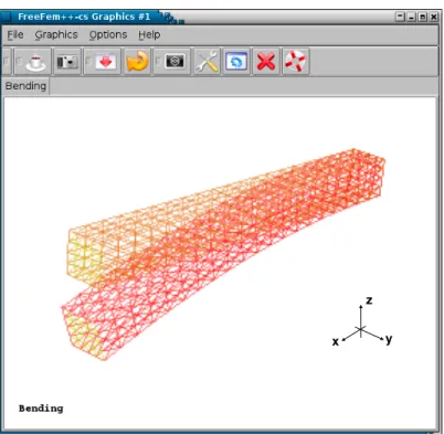
Figure 3.3: FreeFem++implementation of the finite element method in 3D static linear elasticity problem in beam shows the initial mesh and distorted mesh after bending, respectively.
wheref =0is the body force andgis the boundary force on the boundaryΓ. The Lam´e coefficients λ,µare related to the better known constantsE, Young’s modulus, andν, Poisson’s ratio:
µ= E
2(1 +ν) , λ=
Eν
(1 +ν)(1−2ν) . (3.24)
In this case, the mechanical characterization parameter are given as
E = 20×103P a , ν = 0.2 . (3.25)
automatically generated by FreeFem++, with the number of vertices on the edges Nx = 501, Ny = 11andNz = 11alongx-,y- andz-direction, respectively. Thus, after discretization, the total number of node isN =Nx×Ny×Nz = 60621, and the degrees of freedom is3N = 181863. Stretching.The boundary force is the stretching force alongx-directiong= [gx,0,0]T.
Stretching
Figure 3.4: Initial mesh(light) and distorted mesh after stretching (dark), respectively.
Shearing. The boundary force is the shearing force alongy-directiong= [0, gy,0]T.
Shearing
Figure 3.5: Initial mesh(light) and distorted mesh after shearing (dark), respectively.
Bending. The boundary force is the distributed force alongx-directiongi = [gxi,0,0]T providing a bending moment at the free end of the beam.
Bending
Figure 3.6: Initial mesh(light) and distorted mesh after bending (dark), respectively.
3.4.2 Euler-Bernoulli beam theory
Euler-Bernoulli beam theory is a simplification of the linear theory of elasticity which provides a means of calculating the load-carrying and deflection characteristics of beams. The Simplifications on 3D linear system of elasticity are: 1. Averaging the deformations of the material
Neutral axis x
z
w(x) q(x)
Figure 3.7: A single 2D Euler-Bernoulli beam element of two nodes, with three degrees of freedom at each node, two translationsu,v and one rotationθ, is used to represent the 3D linear system of elasticity.
points in 3D linear system of elasticity onto their neutral axis on thexzplane. The neutral axis is straight in its unloaded configuration. The beam is modeled as a one-dimensional object now, and the loadq(x)are normal to the beam axis as shown in Fig (3.7). 2. The material points in 3D linear system of elasticity on the normal to the neutral axis remain on the normal during the deformation. Thus, the deformation of the material points on the normal to the neutral axis can be represented by a rotation angleθ,
θ= dw(x)
dx , θ
0
= d 2w(x)
whichw(x)describes the deflection of the beam in thez-direction at some positionxandκis the curvature of the deflected neutral axis. Eqn (3.26) are called kinematic equations. For a uniform static beam, the Euler-Bernoulli equation describing the relationship between the beam’s deflection and the applied load is given by
EId
4w(x)
dx4 =q(x), (3.27)
whereI is the second moment of area of the beam’s cross-section, andEI is the flexural rigidity. And the constitutive equation, which is a moment-curvature relation assuming a linear distribution of strains and stresses across the cross section, is
M =EIκ. (3.28)
The weak form for finite element discretization is
EI
Z
Ωe
κ(x)κ(v)dx=
Z
Ωe
q(x)vdx (3.29)
For each element of two nodes, the deflectionvalongz-direction and the rotationθdescribe the displacement of the Euler-Bernoulli beam element,
u= [v1, θ1, v2, θ2]T
Introducing the Hermite shape functionsNi (i= 1,· · ·4)interpolations of the displacements into the weak form gives the element stiffness matrix of Euler-Bernoulli beam element,
Ke=EI
Z
Ωe
where the components in the stiffness matrixKije =EIRΩe d2Ni
dx2
d2Nj
dx2 dx. In matrix form,
Ke=
12EI L3 e 6EI L2 e − 12EI L3 e 6EI L2 e 6EI L2 e 4EI Le − 6EI L2 e 2EI Le
−12EI
L3 e − 6EI L2 e 12EI L3 e − 6EI L2 e 6EI L2 e 2EI Le − 6EI L2 e 4EI Le , (3.31)
whereLeis the length of the Euler-Bernoulli beam element.
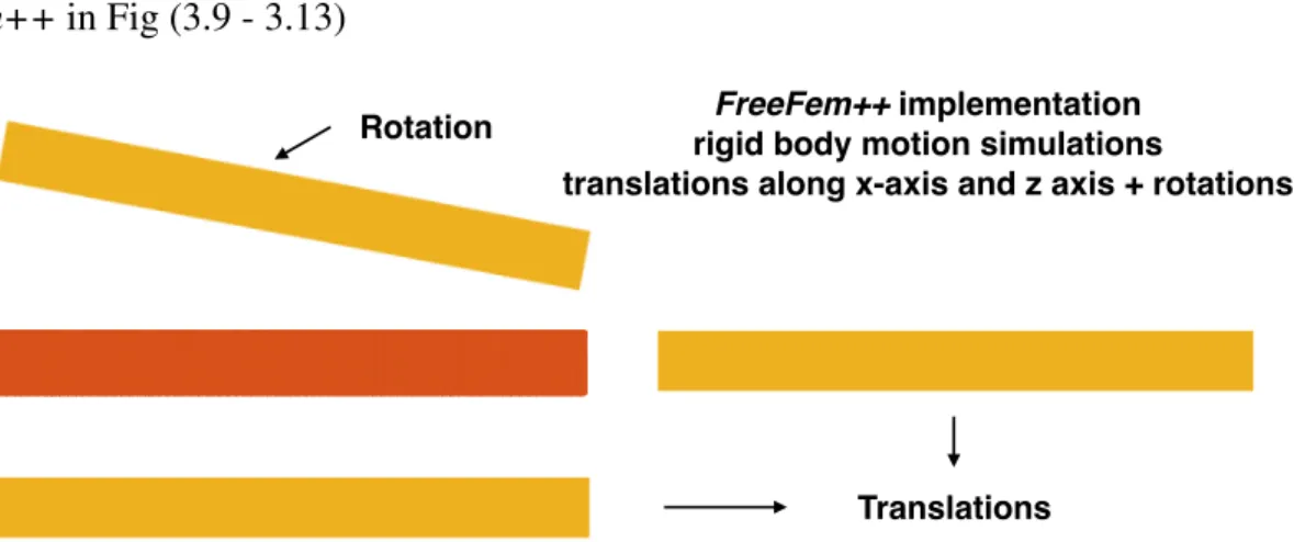
Further, the original 3D linear system of elasticity can be reduced to a single 2D Euler-Bernoulli beam element of two nodes, with three degrees of freedom at each node, two translations u,v and one rotationθ, as shown in Fig (3.8),
u= [u1, v1, θ1, u2, v2, θ2]T.
3D linear system of elasticity 2D Euler-Bernoulli beam element
v1 u1 θ2 u2 v2 θ1 1 2
Figure 3.8: A single 2D Euler-Bernoulli beam element of two nodes, with three degrees of freedom at each node, two translationsu,v and one rotationθ, is used to represent the 3D linear system of elasticity.
(3.31) together,
KeEuler=
EA
Le 0 0 −
EA
Le 0 0
0 12LEI3
e
6EI L2
e 0 −
12EI L3 e 6EI L2 e
0 6LEI2
e
4EI
Le 0 −
6EI L2 e 2EI Le −EA
Le 0 0
EA
Le 0 0
0 −12EI L3 e − 6EI L2 e 0 12EI L3 e − 6EI L2 e
0 6LEI2
e
2EI
Le 0 −
6EI L2 e 4EI Le , (3.32)
where Ke
Euler ∈ R6
×6 is the stiffness matrix of 2D Euler-Bernoulli beam element, with the
mechanical characterization parameter, Young’s modulus E = 20×103 Pa, and the geometric
parameters, the area of cross sectionA= 1m2, the lengthLe = 10m and the second moment of areaI = 121 m4.
Now, the original 3D linear system of elasticity with3N = 181863degrees of freedom is reduced to a 2D Euler-Bernoulli beam element withn = 6degrees of freedom. The stiffness matrixKe
Eulerin Eqn (3.32) can be easily calculated once the mechanical characterization parameter
Young’s modulusEis known.
3.4.3 Model reduction on 3D static linear elasticity problem 3.4.3.1 POD modes of 3D linear system of elasticity
For this 3D static linear elasticity problem of3N = 181863degrees of freedom,m= 60
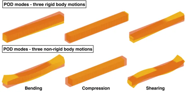
simulations,20stretching/compression simulations (Fig (3.9)),20shearing simulations (Fig (3.10)) and20bending simulations (Fig (3.13)), are computed by usingFreeFem++implementation. All the loads are imposed only onxzplane, thus the corresponding deformations are in the plane, due to the isotropic and homogenous properties of the linear elasticity.
20 19 18 17 16 15 14 13 12 1
1 10
FreeFem++ implementation
stretching/compression simulations - 20 runs
9 8 7 6 5 4 3 2 1
Compression Stretching
Figure 3.9: FreeFem++implementation of stretching/compression simulation on 3D linear system of elasticity. Initial mesh (orange, dark) and distorted mesh (yellow, light), respectively.
20 19 18 17 16 15 14 13 12 1
1 10
FreeFem++ implementation
shearing simulations - 20 runs
Initial configuration
Deformed configuration
9 8 7 6 5 4 3 2 1
20 19 18 17 16 15 14 13 12 1
1 10
FreeFem++ implementation bending simulations - 20 runs
Initial configuration
Deformed configuration
9 8 7 6 5 4 3 2 1
θ
Figure 3.11: FreeFem++implementation of bending simulation on 3D linear system of elasticity. Initial mesh (orange, dark) and distorted mesh after bending (yellow, light), respectively.
The outputs ofFreeFem++implementation are used to form the columns of a snapshot matrix
U=
u1, · · · , u20, u21, · · · , u40, u41, · · · , u60
(3.33) = u1
1 · · · u120 u121 · · · u140 u141 · · · u160
..
. · · · ... ... · · · ... ... · · · ...
u3N
1 · · · u320N u321N · · · u403N u341N · · · u360N
3N×m
, (3.34)
and the corresponding external force matrix
Fext =
fext
1 , · · · , f20ext, f21ext, · · · , f40ext, f41ext, · · · , f60ext
3N×m
. (3.35)
The columns of theUandFextare the deformationsu
i subjected to external forcesFexti computed
by using FreeFem++ implementation.
By using the method of snapshot, instead of SVD on this3N ×mproblem directly, the correlation matrixC ∈Rm×m is formed
This matrix can be factorised, using eigenvalue decomposition, as
C=VΛVT, (3.37)
where the columns ofV = [v1,v2,· · · ,vm]∈ Rm×m, denoted byVj forj = 1,· · · , m, are the
eigenvectors ofCand these will be used as the POD modes,
vpod,j = 1
p
λj
Uvj. (3.38)
In addition,Λ=diag (λ1, λ2,· · · , λm) is the diagonal matrix containing the eigenvalue ofC, which
indicate the relative importance of each modes.
10
20
30
40
50
60
i
th10
-5010
-4010
-3010
-2010
-1010
0log(
i
/sum(
i
) )
Figure 3.12: The log plot of the importance of eigenvalueλi, Pmλi
i=1λi, of correlation matrixC. The
first three modes are the most dominant modes.