Modified Algorithm for Solving Linear Integro Differential Equations of the Second Kind

http://www.scirp.org/journal/ajcm ISSN Online: 2161-1211

ISSN Print: 2161-1203

Modified Algorithm for Solving Linear

Integro-Differential Equations of the

Second Kind

M. Al-Towaiq, Ahmed Kasasbeh

Department of Mathematics and Statistics, Jordan University of Science and Technology, Al Ramtha, Irbid, Jordan

Abstract

In this paper, a modified algorithm is proposed for solving linear inte-gro-differential equations of the second kind. The main idea is based on ap-plying Romberg extrapolation algorithm (REA), on Trapezoidal rule. In ac-cordance with the computational perspective, the comparison has shown that Adomian decomposition approach is more effective to be utilized. The nu-merical results show that the modified algorithm has been successfully applied to the linear integro-differential equations and the comparisons with some existing methods appeared in the literature reveal that the modified algorithm is more accurate and convenient.

Keywords

Algorithm, Integro-Differential Equations, Trapezoidal Rule, Romberg Ex-trapolation

1. Introduction

Mathematical modelling of real-life problems usually results in functional equa-tions, such as differential, integral, and integro-differential equations. Many mathematical formulations of physical phenomena reduced to integro-differen- tial equations, like fluid dynamics, biological models and chemical kinetics [1] [2][3].

The numerical solution of integro-differential equation is a part of numerical analysis, which has been changed by the ongoing revolution in numerical meth-ods. With the development of technology, useful methods are evolving for full utilization of the inherent powers of high speed and large memory computing machine. Many significant methods were discovered to approximate the solution

How to cite this paper: Al-Towaiq, M. and Kasasbeh, A. (2017) Modified Algorithm for Solving Linear Integro-Differential Equa-tions of the Second Kind. American Journal of Computational Mathematics, 7, 157-165. https://doi.org/10.4236/ajcm.2017.72014

Received: May 4, 2017 Accepted: June 19, 2017 Published: June 22, 2017 Copyright © 2017 by authors and Scientific Research Publishing Inc. This work is licensed under the Creative Commons Attribution International License (CC BY 4.0).

of linear integro-differential equations, such as the Improved Bessel collocation method [4], the Legendre wavelets method [5], the finite element method [6], the Tau method [7], Euler polynomials [8], Sherman-Morrison formula [9], the Adomian’s decomposition method [10][11], the Cas wavelet [12], the homotopy perturbation method [13], the Variational iteration method [14] [15] [16], the comined Laplace transform and the Adomian decomposition methods [17], the Sinc method [18] [19], the Galerkin method [20], Romberg extrapolation [21], the Chebyshev polynomial approach [22][23], Lagrange Interpolation [24], and many mathematicians still search to get strong methods and powerful tech-niques to solve problems in integro-differential equations.

Without loss of generality, the linear Fredholmintegro differential equation of the second kind was considered.

( )

( )

b

( ) ( )

, d ,

( )

,

a

u x′ = f x +

∫

k x t u t t u a =

α

(1)

where, α is a real constant.

Some authors studied the numerical solution of the nonlinear integro-differ- ential equations by the Adomian decomposition method and compared it with the variational iteration method [14][15][16]. Therefore, results show that the variation iteration method (VIM) has been successfully employed to obtain the approximate analytical solutions of the nonlinear integro-differential equations. Others solve it through a comparison of the Adomian decomposition method and the wavelet-Galerkin method [20]. From the computational view point, the comparison shows that the Adomian decomposition method is more efficient and easy to use.

Saadati et al. [1], presented numerical method to approximate the integro- differential equations (Volterra, Fredholm) using the Trapezoidal rule. This method based on transforming the first derivative integro-differential equations to a system of algebraic equations.

In [22][23], the Chebyshev polynomial was used to approximate the solution of integral equations, system of higher-order linear Fredholm-Volterra inte-gro-differential equations, and inteinte-gro-differential equations. The main idea of their techniques based on transforming these equations to a system of algebraic equations. They showed that the method has some major advantages: Chebyshev coefficients of the solution are found very easily and this process is very fast. An interesting feature of the method obtained analytical solution in many cases. Many studies have indicated the variational iteration method to solve the linear and nonlinear integro differential equations (Volterra, Fredholm) [3] [14][15] [16][17]. They applied the variational iteration method to approximate the so-lutions of the integro-differential equations. The results show that this method is very effective with low computation time. Also, some authors concluded that the method can be used to find exact solution for some cases.

Fredholm type without any difficulties. In this paper, the solutions of the linear integro-differential equations of different types are studied, analyzed and im-plemented using a modified algorithm based on the Romberg extrapolation techniques.

Jaradat et al.[25] presented an applicability of the Homotopy method to solve Fredholm integro-differential equation. They test the validity and the applicabil-ity of this method, and show that the Homotopy techniques are very powerful to approximate the linear Fredholm integro-differential equations.

Mostafa Nadir and Azedine Rahmoune [26], presented a numerical method to approximate the solution of the linear Volterra integral equations of the second kind, based on Simpson’s rule.

The paper is organized as follows: In Section 2, the proposed technique for solving the linear integro-differential equations is introduced. Some numerical experiments are presented in Section 3. The paper is concluded in Section 4.

2. The Modified Algorithm

In this section, the chosen algorithm is introduced for the solution of Fredholm integro-differential equation of the second kind. First, the Trapezoidal rule is applied to approximate the integral and the finite difference to approximate the derivative in (1), and then Romberg extrapolation is applied to increase the ac-curacy of the solution.

The numerical setting and the approximation of the integral for the Volterra Equation (1) will result in the coefficient matrix of the linear system of equations being a lower triangular one, which is exactly due to the variable upper limit x of the integration in (1), because in this equation the kernel k x t

( )

, ≡0 for t>x

as the integrand can be considered identically zero above it is upper limit of in-tegration x. So, for the discrete case k x t

( )

_i, _j =k_ij =0 for j>i is used. Then the system of linear equations with such a natural triangular coefficient matrix can be solved easily.

To use Trapezoidal rule the interval of integration

(

a x,

)

has been

parti-tioned into n equally spaced subintervals of width

, 1,

n

x a

h n

n

−

= ≥ ₍₂₎

where xn is the end point chosen for x; set t0 = a should be set and

0 , 1, 2, 3, , .

j

t = +a jh= +t jh j=  n (3)

Then the approximation of the integral in the integro-differential Equation (1) is given by,

( ) ( )

(

0

) ( ) ( ) ( )

0 1 1

(

1

) ( )

1

(

) ( )

1 1

, d , , , , ,

2 2

x

n n n n

ak x t u t t h k x t u t k x t u t k x t− u t− k x t u t

 

≅ _ + + + + _

 

∫

 (4)

where,

, , 1, .

j

j n n

t a x a

h t x j x x t

j n

− −

Replace n by 2n m

= _{, then (4) becomes,}

( ) ( )

(

0

) ( ) ( ) ( )

0 1 1

(

1

) ( )

1

(

)

1 1

, d , , , , ,

2 2

x

m m m m

ak x t u t t h k x t u t k x t u t k x t − u t − k x t ut

 

≅ _ + + + + _

 

∫

 (6)

which is called R(n, 0). Then Romberge algorithm (REA) Rk,jcan be applied,

where,

, 1 1, 1

, , 1 , , 1

4 1

k j k j

k j k j j

R R

R R − − − − i j

−

= + ≥

− (7) Now, substitute Equation (6) in (1), thus obtain,

( )

( )

(

0

) ( ) ( ) ( )

0 1 1

(

1

) ( )

1

(

) ( )

1 1

, , , , ,

2 m m 2 m m

u x′ = f x +h_ k x t u t +k x t u t + +k x t ₋ u t ₋ + k x t u t _

   (8)

If n values of ui′=u x′

( )

i =u t′

( )

i are considered and,

( ) ( ) ( ) ( )

, _{j j i}, _{j j} , 1, 2,3, , ,

k x t u t =k x t u t i=  n

then Equation (8) becomes,

( )

( )

(

0

) ( )

0

(

) ( ) ( ) ( )

(

) ( )

1 1 1 1

, ,

, ,

2 2

i i m m

i i i i m m

k x t u t k x t u t

u x′ = f x +h_ + +k x t u t + +k x t ₋ u t ₋ _

   (9)

For simplicity Equation (9) becomes,

, 0 0

1 1 , 1 1 .

2 2

i m m i

i i i

i m m

k u k u

u f h k u k −u −

 

′ = + _ + + + + _

   (10)

The finite difference formula is applied,

( )

3

( )

4

(

) (

2

)

2

u x u x h u x h u x

h

− − + −

′ ≅

to approximate ui′

( )

x in Equation (10) to get the following equation

,

1 2 0 0

1 1 , 1 1

3 4

.

2 2 2

i m m

m m m i

i i u i m m

k u

u u u k u

f h k k u

h − − − −   − + _{= + + + + +}  

   (11)

In matrix notation, Equation (11) transform into the following system of lin-ear equations:

, KU=F

where,

( )

(

)(

)

(

)

(

)(

)(

)

(

)

(

)

(

) (

)

2 2 2 2

11 12 13 1

2 2 2 2 2 2

21 22 23 23 23 12

2 2 2

31 32 33

2 2 2 2

1,1 1,2 1, 1 1,

2 2 2 2

,1 ,2 , 1 ,

1 2 2

2 1 2 1 2 1 2 1 2 2 2 1

2 2 2 1 2

2 2 2 4 2 3

m

m

m m m m m m

m m m m m m

K h k h k h k h k

h k h k h k h k h k h k

h k h k h k

h k h k h k h k

h k h k h k h k

− − − − − −  = −_ − − − − + − − − − − − − + − − − − −  − − − + − _{− }    

 (13)

(

1, 2, , 1,

)

t

m m

And,

(

2

)

(

2

)

2

( )

2

( )

1 10 0 2 20 0 1 1,0 0 1,0 0

2 1 , 2 , , 2 _{m m} , 2 _{m m} t.

F=_ hf + h k + u hf + h k u  hf ₋ +h k ₋ u hf +h k ₋ u _ (15)

This system can be solved for the unknowns ui’s, i=1, 2,,m easily.

3. Numerical Experiments

In this paper, illustrative examples of integro-differential equation are given to demonstrate the accuracy and efficiency of the proposed technique and compare it with some other existing methods.

Example 3.1 [10]. Consider the following Linear Fredholm integro-differential equation of the first derivative:

( )

1

( ) ( )

0

1

1 , 0 0, 3

u x′ = − x+

∫

xtu t u = (16)

In Equation (16),

( )

1

( )

1 , , . 3

f x = − x k x t =xt

The exact solution of Equation (3.1) is:

( )

.

u x =x (17)

The modified algorithm of Romberg extrapolation is applied for solving this example. Following equation is used:

5

1 , 16

h=h = then k=5, with x₀=0, and x16=1, with mesh points,

5, 1, 2, ,16. i

x =ih i=  (18)

Apply Equation (10) and Equation (11) to compute the approximate solution,

, 1, 2, ,16.

i

u i= 

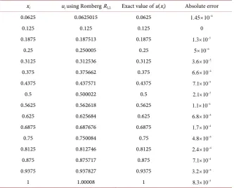
Table 1 shows the absolute errors of the numerical results of R5,2. It is shown

that the proposed algorithm is accurate and efficient. Based on the recursive re-lations of Romberg extrapolation the accuracy increased with less computation time.

In [10], Vahidi reported the computed absolute error for Example (3.1), with

n = 10 for different methods such as the CAS wavelet method, the differential transform method (DTM), and the Adomian decomposition method (ESA). For comparison purposes, norm 2 for the absolute error vector of all the points on [0, 1] is computed. The computed norms for all the above mentioned methods and technique (REA) are shown in Table 2. The table shows that algorithm is more accurate and convenient than other methods. But, if technique is compared with the VIM method, the VIM gives better accuracy.

However, the technique has the advantage, on the time Rk,1 is computed, the

accuracy will increase with less computation as the recursive relation of Rom-berg increases.

[image:6.595.207.541.89.356.2]

Table 1. Approximate solution and absolute errors of Example (3.1), using R5,2. xi ui using Romberg R5,2 Exact value of u(xi) Absolute error

0.0625 0.0625015 0.0625 6

1.45 10× −

0.125 0.125 0.125 0

0.1875 0.187513 0.1875 5

1.3 10× −

0.25 0.250005 0.25 6

5 10× −

0.3125 0.312536 0.3125 5

3.6 10× −

0.375 0.375662 0.375 4

6.6 10× −

0.4375 0.437571 0.4375 5

7.1 10× −

0.5 0.500022 0.5 5

2.1 10× −

0.5625 0.562618 0.5625 4

1.1 10× −

0.625 0.625684 0.625 4

6.8 10× −

0.6875 0.687676 0.6875 4

1.7 10× −

0.75 0.750084 0.75 5

4.8 10× −

0.8125 0.812746 0.8125 4

2.4 10× −

0.875 0.875717 0.875 4

7.1 10× −

0.9375 0.937827 0.9375 4

3.2 10× −

1 1.00008 1 5

8.3 10× −

Table 2. Absolute error.

The method Norm of the absolute errors

REA 3

1.2 10× −

CAS Wavelet 2

3.7 10× −

DTM 1

1.7 10× −

ESA 3

1.1 10× −

( )

1 sin ₀x

( ) ( )

, 0 1,

u x′ = + x+

∫

u t u = − (19)

In Equation (19), f x

( )

= +1 sin ,x k x t

( )

, =1. The exact solution of Equation

(3.3) is

( )

1 3 1

e e cos . 4 4 2

x x

u x = − − − x (20)

The modified algorithm of Romberg extrapolation is applied for solving this example.

The study use 5

1 , 16

h = then, k=5, with x0 =0, and x16=1, with mesh

points,

5, 1, 2, ,16. i

x =ih i= 

Apply Equation (11) to compute the approximate solution u ii, =1, 2,, 6.1

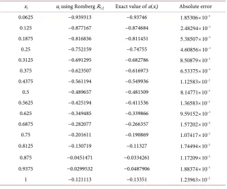
Table 3shows the absolute errors of the numerical results of R5,2. It is shown

time.

In [10], Vahidi reported the computed absolute error for Example 3.2, with n = 10 for the different methods mentioned in example 3.1. The computed norms for all the methods are shown in Table 4. The table shows that the technique is more accurate than the CAS wavelet and the differential transform method (DTM) and has the same accuracy as the Adomian decomposition method (ESA).

4. Conclusion

A modified technique by using Romberg extrapolation on the Trapezoidal rule was introduced to find an approximate solution of the linear integro-differential equation. Some numerical examples appearing in the literature are presented for introducing the main idea behind the approach and for comparisons purposes. The numerical results show that the technique has been successfully applied to the linear integro-differential equations with first derivative. Comparisons with the methods provided in [10] revealed that the technique is more accurate and

Table 3. Approximate solution and absolute errors of Example (3.2) using R5,2. xi ui using Romberg R5,2 Exact value of u(xi) Absolute error

0.0625 −0.939313 −0.93746 3

1.85306 10× −

0.125 −0.877167 −0.874684 3

2.48294 10× −

0.1875 −0.816836 −0.811451 3

5.38507 10× −

0.25 −0.752159 −0.74755 3

4.60856 10× −

0.3125 −0.691295 −0.682786 3

8.50879 10× −

0.375 −0.623507 −0.616973 3

6.53375 10× −

0.4375 −0.561194 −0.549936 2

1.12583 10× −

0.5 −0.489657 −0.481509 3

8.14771 10× −

0.5625 −0.425194 −0.411536 2

1.36583 10× −

0.625 −0.349485 −0.339866 3

9.59152 10× −

0.6875 −0.282077 −0.266357 2

1.57202 10× −

0.75 −0.201611 −0.190869 2

1.07417 10× −

0.8125 −0.130719 −0.11327 2

1.74494 10× −

0.875 −0.0451471 −0.0334261 2

1.17209 10× −

0.9375 −0.0299532 −0.0487906 2

1.88374 10× −

1 −0.121113 −0.13351 2

[image:7.595.207.540.344.620.2]

1.23963 10× −

Table 4. Absolute error.

The method Norm of the absolute errors

REA 3

8.1 10× −

CAS Wavelet 2

7.8 10× −

DTM 1

1.5 10× −

ESA 3

convenient than the other methods. When the technique is compared with the VIM, the VIM normally gives a better accuracy than the method selected. How-ever, the technique has one advantage: the accuracy can be increased with less computation as the recursive relations of Romberg increases.

Acknowledgements

The authors are very thankful to all the associated personnel in any reference that contributed in/for the purpose of this research. Further, this research holds no conflict of interest and is not funded through any source.

References

[1] Saadati, R., Raftari, B., Abibi, H., Vaezpour, S.M. and Shakeri, S. (2008) A Compar-ison between the Variational Iteration Method and Trapezoidal Rule for Solving Li- near Integro-Differential Equations. World Applied Sciences Journal, 4, 321-325. [2] Jerri, A.J. (1999) Introduction to Integral Equations with Applications. John Wiley

& Sons, New York.

[3] Alawneh, A., Al-Khaled, K. and Al-Towaiq, M. (2010) Reliable Algorithms for Solving Integro-Differential Equations with Applications. International Journal of Computer Mathematics, 87, 1538-1554.

https://doi.org/10.1080/00207160802385818

[4] Yuzbas, S. (2016) Improved Bessel Collocation Method for Linear Volterraintegro- Differential Equations with Piecewise Intervals and Application of a Volterra Popu-lation Model. Applied Mathematical Modelling, 40, 5349-5363.

https://doi.org/10.1016/j.apm.2015.12.029

[5] Razzaghi, M. and Yousefi, S. (2005) Legendre Wavelets Method for the Nonlinear Volterra-Fredholm Integral Equations. Mathematics and Computers in Simulation, 70, 1-8. https://doi.org/10.1016/j.matcom.2005.02.035

[6] Sharma, N. and Sharma, K. (2015) Finite Element Method for a Nonlinear Parabo-licintegro-Differential Equation in Higher Spatial Dimensions. Applied Mathemat-ical Modelling, 39, 7338-7350. https://doi.org/10.1016/j.apm.2015.02.037

[7] Pour-Mahmoud, J., Rahimi-Ardabili, M.Y. and Shahmorad, S. (2005) Numerical Solution of the System of Fredholm Integro-Differential Equations by the Tau Me-thod. Applied Mathematics and Computation, 168, 465-478.

https://doi.org/10.1016/j.amc.2004.09.026

[8] Mirzaee, F. and Bimesl, S. (2015) Numerical Solutions of Systems of High-Order Fredholmintegro-Differential Equations Using Euler Polynomials. Applied Mathe-matical Modelling, 39, 6767-6779. https://doi.org/10.1016/j.apm.2015.02.022 [9] Egidi, N. and Maponi, P. (2010) The Use of Sherman-Morrison Formula in the

So-lution of Fredholmintegral Equation of Second Kind. Mathematics and Computers in Simulation, 81, 693-704. https://doi.org/10.1016/j.matcom.2010.03.006

[10] Vahidi, A.R., Babolian, E., Cordshooli, G.A. and Azimzadeh, Z. (2009) Numerical Solution of Fredholm Integro-Differential Equation by Adomian’s Decomposition Method.International Journal of Mathematical Analysis, 36, 1769-1773.

[11] El-Sayed, S.M. and Abdel-Aziz, M.R. (2003) A Comparison of Adomian’s Decom-position Method and Wavelet-Galerkin Method for Solving Integro-Differential Equations. Applied Mathematics and Computation, 136, 151-159.

https://doi.org/10.1016/S0096-3003(02)00024-3

Equa-tions by Using CAS Wavelet Operational Matrix of Integration.Applied Mathema- tics and Computation, 194, 460-466. https://doi.org/10.1016/j.amc.2007.04.048 [13] Yusufoglu, E. (2009) Improved Homotopy Perturbation Method for Solving

Fred-holm Type Integro-Differential Equations. Chaos Solitons Fractals, 41, 28-37. https://doi.org/10.1016/j.chaos.2007.11.005

[14] Wang, S.Q. and He, J.H. (2007) Variational Iteration Method for Solving Integro- Differential Equations. Physics Letters A, 367, 188-191.

https://doi.org/10.1016/j.physleta.2007.02.049

[15] Abbasbandy, S. and Shivanian, E. (2009) Application of Variational Iteration Me-thod for nth-Order Integro-Differential Equations. Zeitschrift für Naturforschung A, 64, 439-444. https://doi.org/10.1515/zna-2009-7-805

[16] Sweilam, N.H. (2007) Fourth Order Integro-Differential Equations Using Varia-tional Iteration Method. Computers & Mathematics with Applications, 54, 1086- 1091. https://doi.org/10.1016/j.camwa.2006.12.055

[17] Wazwaz, A.M. (2010) The Combined Laplace Transform-Adomian Decomposition Method for Handling Nonlinear Volterra Integro-Differential Equations. Applied Mathematics and Computation, 216, 1304-1309.

https://doi.org/10.1016/j.amc.2010.02.023

[18] Rashidinia, J. and Zarebnia, M. (2007) The Numerical Solution of Integro-Diffe- rential Equation by Means of the Sinc Method. Applied Mathematics and Compu-tation, 188, 1124-1130. https://doi.org/10.1016/j.amc.2006.10.063

[19] Kajani, M.T., Ghasemi, M. and Babolian, E. (2006) Numerical Solution of Linear Integro-Differential Equation by Using Sine-Cosine Wavelets. Applied Mathematics and Computation, 180, 569-574. https://doi.org/10.1016/j.amc.2005.12.044

[20] Maleknejad, K. and Kajani, M.T. (2004) Solving Linear Integro-Differential Equa-tion System by Galerkin Methods with Hybrid FuncEqua-tions. Applied Mathematics and Computation, 159, 603-612. https://doi.org/10.1016/j.amc.2003.10.046

[21] Meštrović, M. and Ocvirk, E. (2007) An Application of Romberg Extrapolation on Quadrature Method for Solving Linear Volterra Integral Equations of the Second Kind. Applied Mathematics and Computation, 194, 389-393.

https://doi.org/10.1016/j.amc.2007.04.043

[22] Daşcıoğlu, A. (2006) A Chebyshev Polynomial Approach for Linear Fredholm- Volterra Integro-Differential Equations in the Most General Form. Applied Mathe- matics and Computation, 181, 103-112. https://doi.org/10.1016/j.amc.2006.01.018 [23] Daşcıoğlu, A. and Sezer, M. (2005) Chebyshev Polynomial Solutions of Systems of

Higher-Order Linear Fredholm-Volterra Integro-Differential Equations. Journal of the Franklin Institute, 342, 688-701. https://doi.org/10.1016/j.jfranklin.2005.04.001 [24] Rashed, M.T. (2004) Lagrange Interpolation to Compute the Numerical Solutions of

Differential, Integral and Integro-Differential Equations. Applied Mathematics and Computation, 151, 869-878. https://doi.org/10.1016/S0096-3003(03)00543-5 [25] Jaradat, H., Alsayyed, O. and Al-Shara, S. (2008) Numerical Solution of Linear

In-tegro-Differential Equations. Journal of Mathematics and Statistics, 4, 250-254. https://doi.org/10.3844/jmssp.2008.250.254

Submit or recommend next manuscript to SCIRP and we will provide best service for you:

Accepting pre-submission inquiries through Email, Facebook, LinkedIn, Twitter, etc. A wide selection of journals (inclusive of 9 subjects, more than 200 journals)

Providing 24-hour high-quality service User-friendly online submission system Fair and swift peer-review system

Efficient typesetting and proofreading procedure

Display of the result of downloads and visits, as well as the number of cited articles Maximum dissemination of your research work

Submit your manuscript at: http://papersubmission.scirp.org/