On the Application of Bootstrap Method to
Stationary Time Series Process
T. O. Olatayo
Mathematical Sciences Department, Olabisi Onabanjo University, Ago-Iwoye, Nigeria Email: [email protected]
Received October 15, 2012; revised December 3, 2012; accepted December 14,2012
ABSTRACT
This article introduces a resampling procedure called the truncated geometric bootstrap method for stationary time se-ries process. This procedure is based on resampling blocks of random length, where the length of each blocks has a truncated geometric distribution and capable of determining the probability p and number of block b. Special attention is given to problems with dependent data, and application with real data was carried out. Autoregressive model was fitted and the choice of order determined by Akaike Information Criterion (AIC) and Bayesian Information Criterion (BIC). The normality test was carried out on the residual variance of the fitted model using Jargue-Bera statistics, and the best model was determined based on root mean square error
MSE
of the forecasting values. The bootstrap method gives a better and a reliable model for predictive purposes. All the models for the different block sizes are good. They preserve and maintain stationary data structure of the process and are reliable for predictive purposes, confirming the efficiency of the proposed method.Keywords: Truncated Geometric Bootstrap Method; Autoregressive Model; Akaike Information Criterion (AIC);
Bayesian Information Criterion (BIC); Root Mean Square Error
MSE
1. Introduction
The heart of the bootstrap is not simply computer simu-lation, and bootstrapping is not perfectly synonymous with Monte Carlo. Bootstrap method relies on using an original sample or some part of it, such as residuals as an artificial population from which to randomly resampled [1]. Bootstrap resampling methods have emerged as powerful tools for constructing inferential procedures in modern statistical data analysis. The Bootstrap approach, as initiated by [2], avoids having to derive formulas via different analytical arguments by taking advantage of fast computers. The bootstrap methods have and will con-tinue to have a profound influence throughout science, as the availability of fast, inexpensive computing has en-hanced our abilities to make valid statistical inferences about the world without the need for using unrealistic or unverifiable assumptions [3].
An excellent introduction to the bootstrap maybe found in the work of [4-9]. Recently, [10,11] have inde-pendently introduced non-parametric versions of the bootstrap that are applicable to weakly dependent sta-tionary observations. Their sampling procedure have been generalized by [12,13] and by [14] by resampling “blocks of blocks” of observations to the stationary time
series process.
In this article, we introduce a new resampling method as an improvement on the stationary bootstrap of [15] and the moving block bootstrap of [16,17].
The stationary bootstrap is essentially a weighted av- erage of the moving blocks bootstrap distributions or estimates of standard error, where the weights are deter-mined by a geometric distribution. The difficult aspect of applying these methods is how to choose b in moving blocks scheme and how to choose p in the stationary scheme.
On this note we propose a stationary bootstrap method generated by resampling blocks of random size, where the length of each block has a “truncated geometric dis- tribution”.
In Section 2, the actual construction of a truncated geometric bootstrap method is presented. Some theoreti- cal properties of the method are investigated in Section 3 in the case of the mean. In Section 4, it is shown how the theory may be extended to stationary time series proc- esses.
2. Material and Method
geo-metric stationary scheme in determining both b (number of blocks) and p (probabilities). We introduced a trun-cated form for the geometric distribution and then dem-onstrated that it is a suitable model for a probability problem. This truncation is of more than just theoretical interest as a number of application has been reported [18,19].
A random length L may be defined to have a truncated geometric distribution with parameter P and N terms, when it has the probability distribution or probability density function
11 r , 1, 2, ,
P Lr K P P r N (2.1) The constant K is found, using the condition
1P Lr
, to be 1 1
1
NP
Thus, we have
1
1
1, 2,3, ,
1 1
r N
P P
P L r r N
P
(2.2)
These are the probabilities of a truncated geometric distribution with parameter P and N terms. Suppose that L length, number 1 to N are to be selected randomly with replacement. Then, the process continues until it is trun-cated geometrically at r with an appropriate probability P attached to its random selection in form of ,r r1,
. We take our N to be 4, that is, the ran-dom selections could be truncated between 1 to 4 at an appropriate probabilities.
2, 1
r rN
Then, a description of the resampling algorithm when r > 1 is as follows:
1) Let X1, , XN be a random variables.
2) Let X1 be determined by the r-th truncated ob-servation Xr in the original time series.
3) Let Xi 1
be equal to Xr+1 with probability 1 – P
and picked at random from the original N observations with probability p.
4) Let 1 , be the block con-sisting of b observation starting from Xi.
, , 1, ,
i b i i i b
B X X X
5) Let 1 1, 2, 2 be a sequence of blocks of ran-dom length determined by truncated geometric distribu-tion.
, ,
I L I L
B B
6) Thefirst L1, observations in the pseudo time series
1, 2, , N
X X X are determined by the first block 1 1,
I L
of observation 1 1 1
i
I IL the next L2observations
in the pseudo time series are the observations in the sec-ond sampled block
B ,
, , ;
X X
.
I L
X221 .
7) The process is resampled with replacement, until the process is stopped once N observation in the pseudo time series have been generated.
8) Once X1, ,XN
has been generated, one can compute the quantities of interest for the pseudo time series.
The algorithm has two major components, the
con-struction of a bootstrap sample and the computation of statistics on this bootstrap sample, and repeat these op-eration many times through some kinds of a loop.
Proposition 1. Conditional on X X1, 2, , XN, 1, 2, , N
X X X is stationary.
If the original observations X1, , XN are all distinct, then the new series X1, ,XN
is, conditional on X1,,
N
X a stationary Markov chain. If, on the other hand, two of the original observations are identical and the re-maining are distinct, then the new series X1, ,XN
is a stationary second order Markov chain. The stationary bootstrap resampling scheme proposed here is distinct from the proposed by [20] but posses the same properties with that proposed by [21].
3. Result and Discussion
In this section, the emphasis is on the construction of valid inferential procedures for stationary time series data, and some illustrations with real data are given. The real data are the geological data from demonstratigraphic data from Batan well at 30 m regular interval, [22]. The data is the principal oxide of sand or sandstone, which is SiO2
or silicon oxide. The point is that the bulk of oil reservoir rocks in Nigeria sedimentary basins is sandstone and shale, a product of sill stone [23]. In other to improve on the geological analysis and prediction of the presence of these elements, a mathematical tool which can be used to examine a wide range of data sets is developed to detect and improve new and old oil basins.
The geological data of 130 observations was subjected to our new method described in section two of this article at 500 and 1000 bootstrap replicates, for block of (1, 2, 3, and 4).
The replicates with minimum variance was selected in each case of number of bootstrap replicates.
3.1. Model Fitting, Normality Test and Forecasting
The linear models are fitted and consider the choice of the order of the linear model on the basis of Akaike In-formation Criterion (AIC), Bayesian InIn-formation Crite-rion (BIC) and residual variance
2 ,
Fitting of AR Models to Bootstrapped Data
[24].
The linear models were fitted to the bootstrapped ob-servations when the bootstrap replicates are (B = 500, B = 1000) for blocks of (1, 2, 3 and 4). When B = 500 rep-licates, we have the following models.
Block 1:
It is found that AIC and BIC is minzimum at P = 4. The fitted model is
1 2
3 4
0.373717 0.089415 0.284547 0.248579
t t t
t t
X X X
X X
t
Block 2:
The fitted model is:
1 2
4 5
0.38859 0.030660 0.315254 0.023246 0.300233
t t t
t t t
3
t
X X X
X X X 3 t (3.2) Block 3:
The model fitted is:
1 2
4 5
0.539969 0.070547 0.101612 0.182896 0.101372
t t t
t t t
X X X
X X X 2 t (3.3) Block 4:
The fitted model is:
1
3 4
0.514047 0.099161 0.16566 0.218808
t t t
t t
X X X
X X
(3.4)
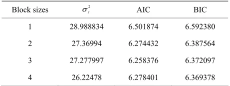
The table below shows the value of 2
, AIC and BIC
for blocks (sizes) when B = 500 replicates. When B = 1000 replicates
Block 1:
The fitted model is:
1 2
4 5
0.166656 0.136937 0.277032 0.238011 0.177745
t t t
t t t
3
t
X X X
X X X t t (3.5) Block 2: 1 2 3 4 0.175163 0.130792 0.414360 0.276122
t t t
t t
X X X
X X
(3.6)
Block 3:
The fitted model is:
1 2 3 0.607054 0.100892 0.289670 t t t t
X X X
X 3 t (3.7) Block 4:
The fitted model is:
1 2
4 5
0.480194 0.14219 0.09358 0.08590 0.196596
t t t
t t t
X X X
X X X (3.8)
The table below summarizes the value of 2
, AIC
and BIC for blocks (sizes) when B = 1000 replicates. From Tables 1 and 2, it observed that the residual
variance
2 for each block sizes are moderate,
indi-cating a selection procedure from any of the models re-tain the time series data structure and any prediction from it is reliable.
3.2. Normality Test for Residual of Fitted Models
[image:3.595.58.291.72.551.2]An important assumption we have made in fitting the linear and non-linear models to data is that the error
t of the model are mutually independent and normal. If a model is fitted to some data it may be appropriate to seeTable 1. Measure of goodness fit by block sizes for 500 rep-licates.
Block sizes 2
AIC BIC
1 28.988 34 8 6.501874 6.592380
2 27.36994 6.274432 6.387564
3 27.277997 6.258376 6.372097
4 26.22478 6.278401 6.369378
able 2. Measures of goodness of fit by block sizes for 1000 T
replicates.
Block sizes 2
AIC BIC
1 28.836 6 84 6.226858 6.39991
2 35.983489 6.618683 6.708724
3 23.631109 6.153097 6.220627
4 23.335846 6.373635 6.487951
ne can consider the model suitable for forecasting. car-rie
o
The normality test for residuals of fitted models is d out using Jargue-Bera statistic tests (JB). At 5% level of significance with 2 degree of freedom the critical values of 2
2
is 5.99, (15) So, if JB > 5.99, one rejects the null hy hesis that the test is normal.
Test for AR models of 500 replicates
pot
H0: The test is normal
H1: The test is not normal
st is normal in all the block si
for AR models of 1000 replicates
test is normal in all block si
fore, the normality test carried out in this article re
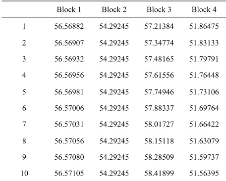
3.3. Forecasting
e fitted and then prediction or
replication of different bl
Table 3 reveals that the te
zes.
Test
H0: The test is normal
H1: The test is not normal
Table 4 reveals that the
zes. There
veals that the proposed truncated geometric bootstrap method for dependent data at different replications is normal in all block sizes and any forecast from this mod-els are good. That is, the residual of the modmod-els satisfied the normality test.
The linear models ar
cast are calculated for the next 10 observations. The fol-lowing are the forecast values for 500 and 1000 repli-cates of different block sizes.
The forecast values for the
ock sizes from the Tables 5 and 6 reveals that while
[image:3.595.308.538.111.197.2] [image:3.595.308.537.236.321.2]Table 3. Summary for JB statistics, B = 500.
Block sizes Skewness Kurtosis Jargue Bera (JB) Probability
1 −0.596584 3.297491 875792. 4 0.019489
2 −0.287789 3.435616 2.713813 0.257456
3 0.183413 4.017238 3.041558 0.048763
[image:4.595.58.285.104.193.2]4 0.195776 3.592815 2.607836 0.271466
Table 4. Summary for JB statistics, B = 1000.
Block sizes Skewness Kurtosis Jargue Bera (JB) Probability
1 −0.191209 3.264664 126511. 5 0.569351
2 −1.856469 3.18611 2.170996 0.00001
3 −0.106644 3.900867 2.499526 0.105424
[image:4.595.308.539.120.202.2]4 −0.121545 3.305079 0.779851 0.677107
Table 5. Forecast values for B = 500 replicates.
Block 1 Block 2 Block 3 Block 4
1 54.98761 55.11951 53.26209 55.72750
2 55.00491 55.13013 53.28615 55.68843
3 55.02221 55.14074 53.31022 55.64935
4 55.03958 55.15136 53.33428 55.61028
5 55.05680 55.16197 53.35834 55.57120
6 55.07410 55.17259 53.38240 55.53213
7 55.09140 55.18321 53.40647 55.45398
8 55.10870 55.19382 53.43053 55.45398
9 55.12600 55.20444 53.45459 55.41490
[image:4.595.57.285.224.312.2]10 55.14330 55.21505 53.47865 55.37583
Table 6. Forecast values for B = 1000 replicates.
Block 1 Block 2 Block 3 Block 4
1 56.56882 54.29245 57.21384 51.86475
2 56.56907 54.29245 57.34774 51.83133
3 56.56932 54.29245 57.48165 51.79791
4 56.56956 54.29245 57.61556 51.76448
5 56.56981 54.29245 57.74946 51.73106
6 56.57006 54.29245 57.88337 51.69764
7 56.57031 54.29245 58.01727 51.66422
8 56.57056 54.29245 58.15118 51.63079
9 56.57080 54.29245 58.28509 51.59737
10 56.57105 54.29245 58.41899 51.56395
Table 7. Root mean square error
MSE
, for t stck sizes
he foreca value.
Blo MSE B, 500 MSE B, 1000
1 6.27811 5.459141
2 7.53356 6.702136
3 7.60897 6.605979
4 6.40647 5.033949
, that shows upward values throughout the period. one 3
In order to justify the best model for prediction, must consider the root mean square error
MSE
of the forecast values. Table 7 is some of root mean squareerror of the forecast values.
To measure and establish the best model, we use the root mean square error of the forecast values. The above table reveals that the values are moderate for all the models in all bootstrap replicates. Therefore models fit-ted for all block of sample sizes are the best model for prediction purposes.
4. Summary and Conclusions
hod proposed in
REFERENCES
[1] G. A. Bancro . Gillet, “A Trun-
The truncated geometric bootstrap met
this article is able to determine P in (0, 1) and provides b, for stationary time series process.
We proposed an algorithm for effective truncated geometric bootstrap method, which shares the construc-tion of resampling blocks of different sizes of observa-tion to form pseudo-time series, so that the statistics of interest are calculated along based on the resampled data sets. We implemented this method with real geological data and generated bootstrap replications of (B = 500 and 1000) for different block sizes of (b = 1, 2, 3, 4) which represents each number of truncations.
The linear models of AR (10) are fitted to the resam-pled pseudo-time series data, and the choice of the order are determined by AIC and BIC. The normality test was carried out using Jargue Bera statistic on the residual variance of the fitted models. Forecast was generated for the next 10 observations based on the fitted models, which are justified by root mean square error of the models.
In conclusion, the bootstrap method gives a better and a reliable models for predictive purposes. All the models for the different block sizes are good. They preserve and maintain stationary data structure of the process and are reliable for predictive purposes, confirming the effi-ciency of the proposed method.
[image:4.595.56.285.340.521.2] [image:4.595.57.285.550.733.2]cated Poisson Distribution,” The Mathematical Gazette, Vol. 67, No. 441, 1983, pp. 216-218. doi:10.2307/3617187 [2] H. Barreto and F. M. Howland, “Introductory Economet-
rics, Using Monte Carlo Simulation with Microsoft Ex- cel,” Cambridge University Press, Cambridge, 2005. doi:10.1017/CBO9780511809231
[3] D. Brillinger, “Time Series: Data Analysis and Theory,”
y, “Bootstrap Methods
omano, “A Review of Bootstrap Con-
t the Jack-Holen-Day, San Francisco, 1981.
[4] A. C. Davison and D. V. Hinkle
and Their Application,” Cambridge University Press, Cambridge, 1997.
[5] T. Diciccio and J. R
fidence Intervals (with Discussion),” Journal of the Royal Statistical Society, Vol. 50, 1988, pp. 338-370.
[6] B. Efron, “Bootstrap Methods Another Look a
nife,” Annals of Statistics, Vol. 7, No. 1, 1979, pp. 1-26.
doi:10.1214/aos/1176344552
[7] B. Efron and R. Tibshirani, “Bootstrap Measures for Stan- dard Errors, Confidence Intervals, and Other Measures of Statistical Accuracy,” Statistical Science, Vol. 1, No. 1, 1986, pp. 54-77. doi:10.1214/ss/1177013815
[8] B. Efron and R. Tibshirani, “An Introduction to the
Boot-e Royal
ting the
tstrap for Gen-strap,” Chapman and Hall/CRC, London, 1993. [9] D. Hinkley, “Bootstrap Method,” Journal of th
Statistical Society, Vol. 50, 1988, pp. 321-337. [10] C. H. Kapadi and R. L. Thomasson, “On Estima
Parameter of the Truncated Geometric Distribution by the Method of Moments,” Annals of the Institute of Statistical Mathematics, Vol. 20, 1975, pp. 519-532.
[11] H. R. Kunsch, “The Jacknife and the Boo
eral Stationary Observations,” The Annals of Statistics, Vol. 17, No. 3, 1989, pp. 1217-1241.
doi:10.1214/aos/1176347265
[12] C. Leger, D. Politis and J. Romano, “Bootstrap Technol- ogy and Applications,” Technometrics, Vol. 34, No. 4, 1992, pp. 378-398. doi:10.1080/00401706.1992.10484950 [13] R. Y. Liu and K. Singh, “Moving Blocks Jackknife and
Bootstrap Capture Weak Dependence,” In: R. Lepage and L. Billard, Eds., Exploring the Limits of Bootstrap, John Wiley, New York, 1992.
[14] J. I. Nwackukwu, “Organic Matter, the Source of Our
, T. O. Olatayo and O. O. Alabi, “Forecasting in
ju, “Rocks: Their Beauty, Language and
l Resampling Sche- Wealth,” An Inaugural Lecture Delivered at Oduduwa Hall, Obafemi Awolowo, University of Ile-Ife, Ile-Ife, 2007.
[15] J. F. Ojo
Subsets, Autoregressive Models and Autoprojective Mo- des,” Asian Journal of Scientific Research, Vol. 1, No. 5, 2008, pp. 1-11.
[16] V. O. Olanrewa
Roles as Resources of Economic Development,” An In- augural Lecture Delivered at Oduduwa Hall, Obafemi Awolowo University, Ile-Ife, 2007.
[17] D. Politis and J. Romano, “A Genera
me for Triangular Arrays of -Mixing Random Variables with Applications to the Problem of Spectral Density Es- timation,” The Annals of Statistics, Vol. 20, No. 4, 1992, pp. 1985-2007. doi:10.1214/aos/1176348899
[18] D. Politis and J. Romano, “A Nonparametric Resampling
Romano, “The Stationary Bootstrap,”
. Lai, “Bootstrap Confidence Procedure for Multivariate Confidence Regions in Time Series Analysis, in Computing Science and Statistics,” In: C. Page and R. Lepage, Eds., Proceedings of the 22nd Symposium on the Interface, Springer-Verlag, New York, 1992, pp. 98-103.
[19] D. Politis and J.
Journal of American Statistical Association, Vol. 89, No. 428, 1994, pp. 1303-1313.
[20] D. Politis, J. Romano and T
Bands or Spectra and Cross-Spectra,” IEEE Transactions on Signal Processing, Vol. 40, No. 5, 1992, pp. 1206- 1215. doi:10.1109/78.134482
[21] M. B. Priestley, “Spectral Analysis and Time Series,”
ality, Strong Mixing
Application with a
urbenko, “The Spectral Analysis of Time Series,” Academic Press, New York, 1981.
[22] M. Rosenblatt, “Asymptotic Norm
and Spectral Density Estimates,” Annals of Probability, Vol. 12, No. 4, 1984, pp. 1167-1180.
[23] K. T. Sofowora, “Factor Analysis:
Chemostratigraphic Data,” Department of Mathematics, Faculty of Science, Obafemi Awolowo University, Ile-Ife, 2002.
[24] I. G. Z