An application of capital allocation principles to operational risk

Munich Personal RePEc Archive

An application of capital allocation

principles to operational risk

Urbina, Jilber and Guillén, Montserrat

Department of Economics and CREIP, Universitat Rovira i Virgili,

Department of Econometrics, Riskcenter-IREA, University of

Barcelona

27 December 2013

Online at

https://mpra.ub.uni-muenchen.de/75726/

An application of capital allocation principles to

operational risk

Jilber Urbinaa,2_{, Montserrat Guill´en}b,1,∗

a_{Department of Economics and CREIP, Universitat Rovira i Virgili, Avinguda de la Universitat 1,}

43204, Reus, Spain.

b_{Department of Econometrics, Riskcenter-IREA, University of Barcelona, Avinguda Diagonal,}

690, E-08034 Barcelona, Spain

Abstract

The cost of operational risk refers to the capital needed to afford the loss generated by ordinary activities of a firm. In this work we demonstrate how allocation prin-ciples can be used to the subdivision of the aggregate capital so that the firm can distribute this cost across its various constituents that generate operational risk. Several capital allocation principles are revised. Proportional allocation allows to calculate a relative risk premium to be charged to each unit. An example of fraud risk in the banking sector is presented and some correlation scenarios between business lines are compared.

Keywords: solvency, quantile, value at risk, copulas

1. Introduction and Motivation

Risk management in business is about anticipating the potential losses that can occur in a firm and to design methods that can either mitigate them or compensate them. It is a field of intense research given that security and protection is an essential part of quality control.

In ordinary business operations, there are risks of malfunctioning that are al-most inevitable and that create a constant burden to the expected profits by sub-stantially reducing those. These risks are called operational because they arise naturally in everyday business activities. They include, software failures, elec-tricity cuts, human mistakes, internal and external fraud, among others. Expected

∗_{Corresponding author}

1_{ICREA Academia and the Ministry of Economy and Competitiveness / FEDER grant}

ECO2010-21787-C01-03 are acknowledged.

2_{This work was developed partly at the Technical University of Catalonia (UPC) and}

operational losses can be accounted for as a fixed cost component of production, but holding a capital to be able to pay for the unexpected operational losses is necessary to respond to exceptional operational risk events that exceed the rou-tine. We will address the cost of operational risk and to what proportion a every single produced unit should contribute to the total capital held for operational risk purposes. A constant allocation would mean that the total capital is divided by the number of product units in spite of the contribution of that unit to the aggre-gate operational risk. A proportional allocation would increase the contribution of those units whose production creates more risk than the others compared to the average.

We will examine an example in the context of fraud in banking. Our illustra-tion is inspired in a typical simplified situaillustra-tion where a bank has only two lines of business, for instance credit cards and savings accounts. Losses due to fraud arise in these two business services and are an area of research for improving business performance [26, 2, 4, 5]. Managers can predict the annual average loss due to fraud in credit cards and savings accounts independently and include this expected loss as part of the general managing expenses of credit cards and savings accounts, respectively. Similar applications have been disussed in the context of automobile insurance before [33]. However, some additional capital must be held as a results of risk exposure due to fraud in any of the two lines and there are several ways to decide how much capital should be provided by the credit card business and how much from the savings account business. Moreover, assuming independence between lines of business is unrealistic. It is well known that fraud propensity fluctuates with exogenous factors that create spurious correlation between busi-ness units [32]. Factors such as economic recession, social networking where people share information about themodus operandiof successful fraud attempts and periods during the year when consumers are more prone to defraud affect all business lines at the same time (see, for instance Caudill et al. [15]). We will address how to cope with dependence between fraud risk in this two dimensional setting, here we consider fraud in credit cards and in savings accounts.

In general, companies wish to allocate capital to their business units for sol-vency reasons. Moreover, banks and insurance companies are legally required to set aside some amount of capital in order to remain solvent and they wish to as-sociate the capital, and therefore the loss of returns, to every single unit as a price loading, also called arisk premium.

The mere existence of operational risk recommends that firms keep some capi-tal, unless they prefer to purchase an insurance policy to cover operations failures, in which case instead of capital they need to pay for an insurance premium, which in our terms is an equivalent problem (see, Guillen et al. [21]).

performance can be assessed by the amount of capital allocated to their business units, which is an indicator of operational risk. Profit-and-loss analysis under loan pricing context and under general investment purposes are another reasons that motivate companies to carry out capital allocations.

Note that capital allocation, namely the contribution to risk of every unit, is the purpose of this work and we do not attempt going into details on how to determine the sum of economic capital to be allocated. We assume this capital is known and given, we are describing a way to determine the optimal proportions of this given capital for allocating them among different risk sources of the enterprise. The main problem to be solved is the so-called allocation problem. Based on the general framework proposed by [16] we provide explicit formulations for the proportion of capitals the manager should allocate on different risk sources based on a wide variety of risk measures.

We provide an exact functional forms of each allocation principle and also paying carefully attention to the numerical part, we analyze the “correlation

ef-fect”on the allocation principles.Correlation effectis considered to be the effect

of changes in the allocated capital suggested by each principle when changing the correlation between the losses. We argue that correlations exist in practice [18, 29, 11, 12]. Our findings suggest thatcorrelation effectexists.

The remainder of this article is arranged as follows. Section 2 discusses for-mally what the allocation problem is. Allocation principles are presented in Sec-tion 3 while the general framework for capital allocaSec-tion, based on [16], is dis-cussed in Section 4. An application is on fraud reported in Section 5. Some concluding remarks are in Section 6.

2. The General Capital Allocation Problem

Capital Allocationis a term referring to the subdivision of the aggregate

cap-ital held by the firm across its various constituents, for example, business lines, type of exposure, territories, or even individual products in a portfolio of insur-ance policies. This capital is often referred to as Economic Capital (EC) and is defined as the p-quantile of the loss distribution minus the expected value of the of loss distribution [28]. Formally, economic capital is a risk measure,

EC(p)= F−_S1(p)−E(S) with,

F_S−1(p)= inf{s∈R_{|FS(s)≥ p}, p∈(0,1).}

and treat it as a more“optimistic”event, this definition states thatECmust be:

ECK =E(S|S > K),

where this definition considers Economic Capital in average also enough to cush-ion losses even in bad times. Note that capital allocatcush-ions in Sectcush-ion 4.2.2 are based on this capital definition.

Once the capital is defined, we have to define its counterpart, i.e. the loss. Consider a portfolio of nindividual losses (random variables)X1,X2, . . . ,Xn ma-terializing at a fixed future dateT. Assume that (X1,X2, . . . ,Xn) is a random vector on the probability space (Ω,F,P_{). We assume that any loss Xi has a finite mean.}

The distribution functionP_{(Xi ≤ x) of Xiwill be denoted byFXi(x).}

The aggregate loss is defined by the sum of the individual losses:

S =

n

X

i=1

Xi, (1)

where this aggregate loss can be interpreted as:

1. the total loss of a corporation, for example, an insurance company, with the individual losses corresponding to the losses of the respective business unit, 2. the loss from an insurance portfolio, with the individual losses being those

arising from the different policies; or

3. the loss by a financial conglomerate, white the different individual losses correspond to the losses suffered by its subsidiaries.

4. the loss of a bank due to fraud in credit card and savings accounts, respec-tively3.

Following [16] it is the first of these interpretations we will use throughout this article. Hence, S is the aggregate loss faced by a company andXi is the loss of business uniti.

In order to clarify what the allocation problem is, one can view the problem from another perspective, namely, consider an investor who can invest in a fixed set of ndifferent investment possibilities with losses represented by the random variablesX1,X2, . . . ,Xn. We have the following economic interpretations depend-ing on the area of application [27]:

1. Performance measurement.Here the investor is a financial institution and

theXi represent the Profit-and-Loss distribution ofndifferent lines of busi-ness.

2. Loan pricing. In this situation the investor is a loan book manager respon-sible for a portfolio ofnloans.

3. General investment. Here we consider either an individual or institutional

investor and the standard interpretation ofXiare profit-and-loss correspond-ing to a set of investments in various assets.

S is random, so usually we assume that the company has already determined the aggregate level of capital safely to face those losses and denote this total risk capital by K. The company now wishes to allocate this exogenously given total risk capitalK across its various business units, that is, to determine non-negative real numbersK1, . . . ,Knsatisfying the full allocation requirement:

n

X

i=1

Ki = K. (2)

This allocation is in some sense a notional exercise; it does not mean that capital is physically shifted across the various units, as the company’s assets and liabilities continue to be pooled. The allocation exercise could be made in order to rank the business units according to levels of profitability. This task can be performed, for example, by determining the returns on the allocated capital for the respective business units.

The general approach of capital allocation raises the question of what the ap-propriate risk capital for an individual investment opportunity might be. Thus the question of performance of the investment is intimately connected with the risk measurement chosen. A two-step procedure is used in practice [27].

1. Compute the overall risk capitalρ(S), whereS is defined in (1) andρ is a particular risk measure, such as value at risk (VaR), expected shortfall (ES), or an economic capital (EC(p)) (see Dhaene et al. [17], ? ], Guillen et al. [22] and Abbasi and Guillen [1] for detailed explanations and applications and Alemany et al. [3] for estimation methods). Coherent measures will be more appropriate than non-coherent ones as they guarantee sub-additivity4 Some new measures have been proposed in this area and they could gener-alize the interpretation [6]

2. Compute K as ρ(S) and allocate the capital K to the individual units ac-cording to some mathematicalcapital allocation principlesuch that, if (Ki) denotes the capital allocated toiwith potential lossXi. The sum ofKifulfills the requirement in (2).

4

We are interested in the second step of the procedure above; roughly speaking we require a mapping that takes as input the individual losses X1,X2, . . . ,Xn and the risk measureρand yields as output the vector (K1,K2, . . . ,Kn) such that:

ρ(S)= n

X

i=1

Ki = K. (3)

Such a mapping is called a capital allocation principle. The relation (3) is sometimes called thefull allocation property[27] since all of the overall risk cap-italρ(S) (not more, not less) is allocated to the investment possibilities; [27] con-sider this property to be an integral part of the definition of an allocation principle. Given that a capital allocation can be carried out in a countless number of ways, additional criteria must be set up in order to determine the most suitable form of determining the mapping. A reasonable start is to require the allocated capital amounts Ki to be “close” to their corresponding losses Xi in some appro-priately defined sense. Prior to introducing the idea of “closeness” between in-dividual loss and allocated capital, we revisit some well-known capital allocation methods.

3. Allocation Principles in Risk Management

A capital allocation principle in risk management is a general rule that assigns a capital K that is aimed to cover an aggregated loss S, to units that contribute to S and not necessarily independently. The reasons why firms want their total capital needs to cover risk to be allocated are [16]:

1. There is a need to redistribute the total (frictional or opportunity) cost asso-ciated with holding capital across various business lines so that this cost is equitably transferred back to the depositors or policyholders in the form of charges.

2. The allocation of expenses across lines of business is a necessary activity for financial reporting purposes.

3. Capital allocation provides for a useful device of assessing and comparing the performance of the different lines of business by determining the return on allocated capital for each line. Comparing these returns allows one to distinguish the most profitable business lines and hence may assist in re-munerating the business line managers or in making decisions concerning business expansions, reductions or even eliminations.

3.1. Haircut allocation principle

This a is straightforward allocation method consisting of allocating the capital

Ki = γF−_Xi1(p), i = 1, . . . ,n to business unit i, where factor γ is chosen such that the full allocation requirement (2) is satisfied. This gives rise to the haircut

allocation principle:

Ki =

K

n

P

i=1

F−1

Xi (p)

F−_Xi1(p), i=1, . . . ,n. (4)

Haircut principle is based on the idea of measuring stand-alone losses using a VaR for a given (fixed) probability level p that is why it is a very common technique among banks and insurance companies. It boils down to a principle of single proportionality.

It should be noted that K is exogenously determined, it is considered as a given value. The capital allocated by this principle does not rely on the structure dependence of the lossesXiof the different business units. [16] consider haircut as a method which is independent of the portfolio context within which the individual losses are embedded, clearly this fact highlights the non-subadditivity property of the VaR.

The two more immediately consequences derived from non-subadditivity in the haircut principle context are: i) The portfolios do not benefit from a pool-ing effect (this is true even beyond haircut scope) and ii) It may happen that the allocated capitalsKi exceed the respective stand-alone capitalsF_Xi−1(p).

3.2. CTE allocation principle (Overbeck type II allocation principle)

CTE principle is based on conditional tail expectation, we call this kind of allocation Overbeck type II allocation principle5. For a given probability level

p∈(0,1), the CTE of the aggregate loss is defined as:

CT Ep[S]=E

h

S|S > F−_XS1(p)i. (5)

expression (5) for a fixed level p, gives the average of the top (1− p) percent losses.

TheCTE allocation principlefor some fixed probability level p ∈ (0,1) has

the form:

Ki =

K CT Ep[S]

EhXi|S > F −1

XS(p)

i

, i=1, . . . ,n. (6)

Unlike thehaircut allocation principle, theCTE principletakes into account the dependence structure of the random losses (X1,X2, . . . ,Xn). Interpreting the event S > F−1

XS(p) as the “the aggregate loss S is large”, we see from (6) that business units with larger conditional expected loss, given that the aggregate loss

S is large, will be penalized with larger amount of capital required than those with lesser conditional expected loss.

3.3. Covariance allocation principle

TheCovariance allocation principletakes the following form:

Ki =

K

Var[S]Cov(Xi,S), i= 1, . . . ,n, (7)

whereCov(Xi,S) is the covariance between the individual loss Xi and the aggre-gate lossS andVar(S) is the variance of the aggregate loss. Because clearly the sum of the individual covariances is equal to the variance of the aggregate loss, the full allocation requirement in (2) is automatically satisfied in this case.

TheCovariance allocation principleas well as the CTE allocation principle

takes into account the dependence structure of the random losses. A nice interpre-tation that arises from the covariance principle is that “business units with a loss that is more correlated with the aggretate loss S are penalized by requiring them to hold a larger amount of capital than those that are less correlated” [16] .

3.4. Proportional allocations

[27] summarizes all the allocation methods explained in the previous sections into what they call Proportional Allocations which is a more general class en-compassing the allocation principles described above. Depending on which risk measureρis chosen for attributing capitalKiis the key for obtaining one of them. This idea is formalized as:

Ki =ωρ(Xi), i=1, . . . ,n, (8)

whereKi is the capital to be allocated to each business uniti, ρ(·) is risk measure and factorω is chosen such that the full allocation requirement in (2) is satisfied, this factor takes the following form:

ω= _n K

P

i=1 ρ(Xi)

, i= 1, . . . ,n. (9)

allocation principles discussed above:

Ki =

K

n

P

i=1 ρ(Xi)

ρ(Xi), i=1, . . . ,n. (10)

4. Optimal Capital Allocations

As we have pointed out above, K is considered to be exogenous; because there are several allocation principles to aggregate capitalK tonpartsK1, . . . ,Kn corresponding to the different business units. [16] claim that “there seems to be a lack of a clear motivation for preferring to choose one over another, although it appears obvious that different capital allocations must in some sense correspond to different questions that can be asked within the context of risk management” and this is the main focus of the [16] becomes a key reference for systematizing capital allocation methods by viewing them as solutions to a particular decision problem. In order to achieve this goal they formulate a decision criterion, such as:

Capital should be allocated such that for each business unit the allocated capital and the loss are sufficiently close to each other [16].

In order to cast this statement in a more formal setting, consider the aggregate portfolio loss S = X1 + . . .+ Xn with aggregate capital K. Once the aggregate capital is allocated, the difference between the aggregate loss and the aggregate capital can be expressed as:

S −K =

n

X

i=1

(Xi−Ki), (11)

where the quantity (Xi − Ki) expresses the loss minus the allocated capital for uniti. It is important to notice that in this setting, the units are cross-subsidizing each other, in the sense that the occurrence of the event “Xk > Kk” does not necessarily lead to “ruin”; such unfavorable performance of subportfolio k may be compensated by a favorable outcome for one or more values (Xl −Kl) of the other units. [16] propose to determine the appropriate allocation by the following optimization problem:

Definition 1. Optimal Capital Allocation Problem Given the aggregate capital

K > 0, determine the allocated capitals Ki, i=1, . . . ,n, from the following

opti-mization problem:

min

K1,...,Kn

n

X

i=1 υiE

"

ζiD

Xi−Ki υi

!#

, such that,

n

X

i=1

where theυiare non-negative real numbers such thatPni=1υi = 1, the ζi are

non-negative random variables such that E(ζi)= 1, and D is a non-negative function.

Each of the component in the general optimal capital allocation problem in (12) are defined as follows:

υi: The non-negative real number υi is a measure of exposure or business vol-ume of theith unit, such as revenue, insurance premium, etc. These scalar quantities are chosen such that they sum to 1. Their inclusion in the

ex-pression D Xi−Ki

υ_i

!

normalizes the deviations of loss from allocated

capi-tal across business units to make them relatively more comparable. At the same time, the υis are used as weights attached to the different values of

E

"

ζiD

Xi−Ki υi

!#

in the minimization problem in (12), in order to reflect the

relative importance of the different business units.

D Xi−Ki

υi

!

: For simplicity, it is first assumed that υi = 1 and also thatζi ≡ 1.

The termsD(Xi−Ki) quantify the deviations of the outcomes of the lossesXi from their allocated capital Ki. Minimizing the sum of the expectations of these quantities essentially reflects the requirement that the allocated cap-itals should be “as close as possible” to the losses they are allocated to. Examples of distance measures are “squared or quadratic deviations” and “absolute deviations”.

ζi The deviations of the losses Xi from their respective allocated capital levels

Ki are measured by the terms EζiD(Xi−Ki). These expectations involve non-negative random variables ζi with E(ζi) = 1 that are used as weight factors to the different possible outcomes ofD(Xi−Ki). One possible choice for the ζi could be ζi = h(Xi) for some non-negative and non-decreasing functionh. In this case, the heaviest weights are attached to deviations that correspond to states of the world leading to the largest outcomes of Xi. We will call allocations based on such a choice for the ζi business unit driven

allocations.

Another choice is to letζi =h(S) for some non-negative and non-decreasing functionh, such that the outcomes of the deviations are weighted with re-spect to the aggregate portfolio performance. In this case, heavier weights are attached to deviations that correspond to states of the world leading to larger outcomes of S. Allocations based on such a choice for the random variablesζiwill be calledaggregate portfolio driven allocations.

weighting is market driven and the corresponding allocation is said to be a

market-driven allocation.

TheQuadratic Optimization Criterion is proposed by [16] as the General

Solution of the Quadratic Allocation Problemby letting

D(x)= x2. (13)

This leads to (12) to

min K1,...,Kn

n

X

i=1

E

"

ζi

(Xi−Ki)2 υi

#

, such that,

n

X

i=1

Ki = K. (14)

The solution to this minimization problem is given in the following theorem.

Theorem 1. The optimal allocation problem in (14) has the following unique

so-lution:

Ki = E(ζiXi)+υi

      K − n X

i=1

E(ζiXj)

     

, i

=1, . . . ,n. (15)

A detailed proof of the solution for this minimization problem can be found in [16].

4.1. Business unit driven allocations

Following [16], in this subsection, we consider the case where the weighting random variablesζiin the quadratic allocation problem in (14) are given by

ζi = hi(Xi), (16)

withhi being a non-negative and non-decreasing function such thatE[hi(Xi)]= 1, fori = 1, . . . ,n. Hence, for each business uniti, the states of the world to which we want to assign the heaviest weights are those under which the business unit performs the worst. As earlier pointed out, we call allocations based on (16) business unit driven allocations. In this case, the allocation rule in (15) can be rewritten as

Ki = E[Xihi(Xi)]+υi

     

K−

n

X

i=1

E[Xihi(Xi)]

     

, i

=1, . . . ,n. (17)

indeed business unit driven. Such allocations might be a useful instrument for determining the performance bonuses of the business unit managers, in case one assumes that each manager should be rewarded for the performance of his own business unit but not extra rewarded (or penalized) for the interrelationship that exists between the performance of his business unit and that of the other units of the company. One should however note that disregarding in this way diversifica-tion between business units, the allocadiversifica-tion may give incentives to managers that are at odds with overall portfolio optimization criteria.

The law invariant risk measureE[Xihi(Xi)] assigns to any lossXithe expected value of the weighted outcomes of this loss, where higher weights correspond to larger outcomes of the loss, that is, to more adverse scenarios. Risk measures and premium principles of this general type are proposed and investigated in [25], [30], and [19].

Defining the volumesυiby

υi =

E[Xihi(Xi)]

Pn

i=1E[Xihi(Xi)]

. (18)

The allocation principle could be found by substituting (18) in (17) and sim-plifying the expression as in:

Ki = E[Xihi(Xi)]+

E[Xihi(Xi)]

Pn

i=1E[Xihi(Xi)]

     

K−

n

X

i=1

E[Xihi(Xi)]

      

Now it can be easily seen from this last expression the allocation principle based on thebusiness unit drivenidea is given by:

Ki =

K

Pn

i=1E[Xihi(Xi)]

E[Xihi(Xi)]. (19)

Once we got to know the general form of the business unit driven allocation principle we are now able to choose different forms forhi(Xi) in order to achieve several capital allocation principles based upon thebusiness unit driven allocation

framework, this is exactly the main purpose of the subsequent sections.

4.1.1. (Pure) Conditional Tail Expectation principle

Once we know the allocation principle for allocating Ki using business unit

driven principlewe can set specific forms forhi(Xi), we can obtain several

explic-itly functional forms forKi, for instance by choosinghi(Xi)=

I_(Xi>F−1

Xi(p))

1−F_Xi(F−1

Xi(p))

, thenKi

We call this principle (Pure) Conditional Tail Expectation because both the aggregate loss and each individual business unit losses are taken conditional ex-pectation based on the average of the top (1− p) loss. SinceCT E(·) is applied to

S andXithen we call it(Pure) Conditional Tail Expectationso that we can distin-guish it from theConditional Tail Expectationprinciple based on [28] which we

callOverbeck type II allocation principlewhich is a special case of theAggregate

Portfolio Driven Allocations, see Section 4.2.

Lemma 1. For an integrable loss X with continuous distribution function, FXand

any p∈(0,1)we have [16],

ESp=

1

1− pE(X: X≥ qp(X))= E(X|X ≥VaRp).

By choosing hi(Xi) =

I(Xi>F−1

Xi(p))

1−F_Xi(F−1

Xi(p))

multiplying by Xi and taking expectations

will lead us to:

E[Xihi(Xi)]= E

      Xi

I_{(Xi > F}−1

Xi(p))

1− p

      

= 1

1−pE[Xi|Xi > F

−1

Xi(p)].

From Lemma 1 the previous expressions reduces to theConditional Tail

Ex-pectation:

E[Xihi(Xi)]=CT Ep[Xi].

Now replacingE[Xihi(Xi)] byCT Ep[Xi] in (19) we have:

Ki =

K

Pn

i=1CT Ep(Xi)

CT Ep(Xi)=

K CT Ep(Pni=1Xi)

CT Ep(Xi).

Pn

i=1CT Ep(Xi)=CT Ep(Pni=1Xi) follows from the additivity proporty of CTE.

HenceKi takes the following form:

Ki =

K

CT Ep(S)

CT Ep(Xi). (20)

4.1.2. Standard deviation principle

The standard deviation principle [14] can be easily obtained by choosing

hi(Xi) = 1+aXi−E_σ(Xi)

it into (19) will have the so-calledstandard deviation principle.

In order to get an expression forKi based upon thestandard deviation

princi-plewe proceed as follows:

E[Xihi(Xi)]=E

"

Xi+a

X2_i −XiE(Xi) σXi

#

=E(Xi)+aσXi.

ForPn

i=1E[Xihi(Xi)] to be explicitly found we proceed as follows:

n

X

i=1

E[Xihi(Xi)]= n

X

i=1

E(Xi)+aσXi

= n

X

i=1

E(Xi)+a n

X

i=1

σXi. (21)

Expression (21) can be simplified to (22) if and only ifCov(Xi,Xj)=0 ∀i,

j

E(S)+aσS, (22)

this follows from the following operations:

n

X

i=1

E(Xi)+a n

X

i=1

σXi = E

       n X

i=1

Xi        +a v t Var        n X

i=1

Xi      

⇔Cov(Xi,Xj)

=0 ∀i, _j

= E(S)+aσS.

Consequently the form taken byKi based upon thestandard deviation

princi-pleis:

Ki =

K E(S)+aσS

E(Xi)+aσXi. (23)

A very interesting relationship betweenOverbeck type I allocation principle

which we will be studied in (4.2.2) and theStandard deviation allocation princi-ple, (32) and (23), respectively, is given by:

Ki =

K E(S)+aφ

E(Xi)+

a

σγ

. (24)

Whereas the standard deviation principleis recovered when setting φ = σS and γ =Cov(Xi,Xi)=Var(Xi)= σ2_Xi.

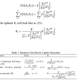
4.1.3. Esscher principle

If we lethi(Xi) be e aXi

E[eaXi] with a > 0 then K will be allocated accordingly by

theEsscher Principle[20], as we shall see below:

E[Xihi(Xi)]=E

"

XieaXi

E[eaXi_]

#

.

n

X

i=1

E[Xihi(Xi)]= n

X

i=1

E

"

XieaXi

E[eaXi_]

#

.

Thus, the optimalKiwill look like as (25):

Ki =

K

Pn

i=1E

"

XieaXi

E[eaXi_]

#E

"

XieaXi

E[eaXi_]

#

. (25)

Table 1: Business Unit Driven Capital Allocation

Reference hi(Xi) Ki

(Pure) Conditional Tail Expec-tation [28]

I(Xi>F_Xi−1(p))

1−F_Xi(F_Xi−1(p)) p∈(0,1)

K

CT Ep(S)CT Ep(Xi)

Standard deviation principle [14]6

1+aXi−E(Xi) σXi

, a≥0 K

E(S)+aσS

E(Xi)+aσXi

Esscher principle [20] eaXi

E(eaXi), a>0 Ki=

K

Pn i=1E

"

XieaXi

E[eaXi_]

#E "

XieaXi

E[eaXi]

#

4.2. Aggregate portfolio driven allocations

Unlike from theBusiness Unit Driven Allocation rule, this time [16] consider the case where

ζi =h(S), i= 1, . . . ,n, (26)

Ki = E[Xih(S)]+υi(K−E[S h(S)]), i=1, . . . ,n. (27)

Hence, the capital Ki allocated to unit i is determined using a weighted ex-pectation of the loss Xi, with higher weights attached to states of the world that involve a large aggregate loss S. Notice that the allocation principle (27) can be reformulated as7

Ki = E(Xi)+Cov[Xi,h(S)]+υi(K−E[S h(S)]), i= 1, . . . ,n. (28)

This means that the capital allocated to theith business unit is given by the sum of the expected loss E[Xi], a loading that depends on the covariance between the individual and aggregate lossesXiandh(S), plus a term proportional to the volume of the business unit. A strong positive correlation between Xi and h(S), which reflects that Xi could be a substantial driver of the aggregate loss S, produces a higher allocated capital Ki.

Using aggregate portfolio driven allocations might be appropriate when one wants to investigate each individual portfolio’s contribution to the aggregate loss of the entire company. In other words, the company wishes to evaluate the sub-portfolio performances, for example, the returns on the allocated capitals, in the presence of the other subportfolios. This can provide relevant information to the company within which it can further be used to evaluate either business expan-sions or reductions.

Defining the volumesυiby

υi =

E[Xih(S)]

E[S h(S)], i=1, . . . ,n. (29) Plugging (29) into (27) and simplifying the resulting expression we end up having a proportional allocation rule:

Ki =

K

E[S h(S)]E[Xih(S)]. (30)

Using the proportional allocation principle shown in (30) and choosing some structure forh(S), the researcher/practitioner can be allowed to construct several ways for allocating K. For instance let us consider a particular choice forh(S) to be h(S) = S − E(S) this yields to the covariance allocation principle intro-duced in section 3 by means of determining the expression for bothE[Xih(S)] and

E[S h(S)] and then plug them into (30) as it is shown below.

7

This follows from the fact that Cov(Xi,h(S)) = E(Xih(S)) − E(Xi)E(h(S)) solving for

4.2.1. Covariance allocation principle

This subsection is intended to derive theCovariance allocation principlefrom the general setting presented in the previous section by setting h(S) = S − E(S) and using the philosophy of theplug-in principle.

Settingh(S)=S −E(S) the aim is to determineE[Xih(S)] andE[S h(S)].

ForE[Xih(S)] we have:

E[Xih(S)]= E[XiS −E(S)] =Cov(Xi,S).

ForE[S h(S)] to be explicitly found we proceed as follows:

E[S h(S)]= E[S(S −E(S))]

= E(S2)−[E(S)]2 =Var(S).

Once we have the expressions forE[Xih(S)] and E[S h(S)] we can now plug them into (30) in order to have the expression for allocating capital K among the different business units (Xi with i = 1, . . . ,n) based on the Aggregate Portfolio

Driven idea. So the allocation principle has the form:

Ki =

K

Var[S]Cov(Xi,S), i= 1, . . . ,n. (31) Precisely this is exactly the expression shown in (7) from this fact one can no-tice thatCovariance Principleis a special case of theAggregate Portfolio Driven

Allocationwhen choosingh(S)=S −E(S).

4.2.2. Overbeck allocation principles

Within this subsection we provide an explicit expression for the Aggregate Portfolio Driven Allocation principle based on [28]. We call Overbeck Type I

allocation principleto the principle obtained by settingh(S)=1+aS−E_σ(S)

S ,a≥ 0. And we will callOverbeck Type II allocation principleto that when usingh(S)=

1

1−pI(S > F −1

S (p)), withp∈(0,1).

As in the previous sections we now proceed to find an explicit expression for

ForE[Xih(S)] we have:

E[Xih(S)]= E

"

Xi 1+a

S −E(S)

σS

!#

= E(Xi)+

a

σS

Cov(Xi,S).

Working onE[S h(S)] we find:

E[S h(S)]= E

"

S + aS(S −E(S))

σS

#

= E(S)+aσS.

Applying theplug-in principleand substituting the respective expressions of

E[Xih(S)] andE[S h(S)] into the general framework presented in (30) we get the allocation principle we’ve just calledOverbeck Type I allocation principlewhose form is:

Ki =

K E(S)+aσS

"

E(Xi)+

a

σS

Cov(Xi,S)

#

. (32)

Overbeck Type II allocation principleis determined by lettingh(S) be_1−p1 I_{(S >}

F_S−1(p)) with p∈(0,1):

E[Xih(S)]= 1

1−pE[Xi|I(S > F

−1

S (p))]

E[S h(S)]= 1

1−pE[S|I(S > F

−1

S (p))]=CT Ep(S).

Therefore,Kicould be written as:

Ki =

K

CT Ep(S)

E[Xi|I(S > F −1

S (p))]. (33)

Note this principle is exactly the same one presented in (6) in Section 3.2

4.2.3. Wang allocation principle

the procedure is similar to the ones used in previous sections.

Once we considerh(S) = _Ee_[eaSaS_], the expression forE[Xih(S)] is found in the following way:

E[Xih(S)]= E

"

S h(S)= e

aS

E[eaS_]

#

= 1

E(eaS₎E(Xie aS₎

= E(Xie aS₎

E(eaS₎ .

ThenE[S h(S)] is:

E[S h(S)]= E

"

Xih(S)=

eaS E[eaS_]

#

= E(S e aS₎

E(eaS₎ .

Therefore, the allocation of the exogenously given aggregate capital K to n

parts K1, . . . ,Kn corresponding to the different business units can be carried out using:

Ki =

K

E(S eaS₎E(Xie

aS_{). (34)}

4.2.4. Tsanaka allocation principle

If we letR₀1 _Ee_(eγaSγaS₎ beh(S) witha>0, then this leads us to the [31] principle. Expressions for constructing theKi are as follow:

E[Xih(S)]= E

"

Xi

Z 1

0

eγaS E(eγaS₎dγ

#

,

E[S h(S)]= E

"

S

Z 1

0

eγaS E(eγaS₎

#

,

where theKi to be allocated takes the following form:

Ki =

K

E

SR1

0

eγaS E(eγaS₎dγ

E

"

Xi

Z 1

0

eγaS

E(eγaS₎dγ

#

LettingΨbeR1 0

eγaS

E(eγaS₎dγ, thenKi could be rewritten as:

Ki =

K

E(SΨ)E(XiΨ). (36)

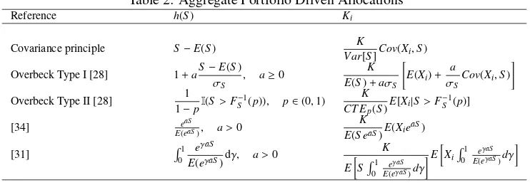
Table 2 summarizes theAggregate Portfolio Driven Allocationsby providing expressions forKi.

Table 2: Aggregate Portfolio Driven Allocations

Reference h(S) Ki

Covariance principle S−E(S) K

Var[S]Cov(Xi,S) Overbeck Type I [28] 1+aS−E(S)

σS

, a≥0 K

E(S)+aσS

"

E(Xi)+ a

σS

Cov(Xi,S)

#

Overbeck Type II [28] 1 1−pI(S>F

−1

S (p)), p∈(0,1) K

CT Ep(S)E[Xi|S>F

−1

S (p)]

[34] eaS

E(eaS₎, a>0

K E(S eaS₎E(Xie

aS₎

[31] R₀1 e

γaS

E(eγaS₎dγ, a>0

K

E

SR₀1 eγaS

E(eγaS₎dγ

E

XiR₀1 eγaS

E(eγaS₎dγ

5. An application to fraud analysis

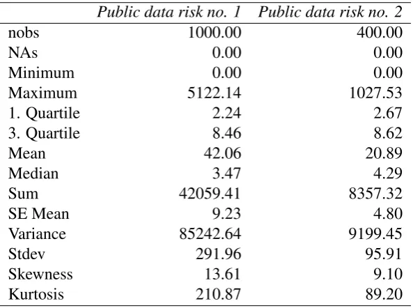
We give the practical examples of capital allocation approaches and their im-pact on amounts of allocated capital when considering a typocal case of opera-tional risk. For this purpose, we usePublic data risk no. 1 andPublic data risk

no. 2 from [8], these data consist of 1000 and 400 observed loss amounts for

categories 1 and 2, respectively.

Let us consider these data as operational losses in a banking environment. For

Public data risk no. 1 to have some sense in this context we consider it as bank

transfer mistakes which means that a bank teller transfers more money than the required to a client’s savings bank account and Public data risk no. 2 is to be considered as fraudulent transactions, for instance, a client loses her credit card and another person uses it, if the bank’s client reports this situation to bank then the non-authorized use of the credit card will charge some losses to bank.

Table 3: Descriptive statistics for numerical example data

Public data risk no. 1 Public data risk no. 2

nobs 1000.00 400.00

NAs 0.00 0.00

Minimum 0.00 0.00

Maximum 5122.14 1027.53

1. Quartile 2.24 2.67

3. Quartile 8.46 8.62

Mean 42.06 20.89

Median 3.47 4.29

Sum 42059.41 8357.32

SE Mean 9.23 4.80

Variance 85242.64 9199.45

Stdev 291.96 95.91

Skewness 13.61 9.10

Kurtosis 210.87 89.20

The reason why we decide to use aggregate portfolio driven allocations is that we want to consider the dependence structure compared to the Haircut allocation principle, which is based on a stand-alone risk measure which does not consider the dependence structure. Dependence structures cannot be ignored in risk man-agement [23, 24].

Some descriptive insights are provided in Table 3 where one eye-catching fact is the difference in the number of observations in each vector of losses, Public

data risk no. 1has 1000 observations and Public data risk no. 2has 400 which

represents a drawback for the configuration of the allocation principles where all of them implicitly assume identical length for vector of losses, we overcome this inconvenient by using two different re-sampling techniques: bootstrapping and an uniformly pairwise random extraction. Another important characteristic of these data is the strong non-normality suggested by the skewness and the kurtosis coefficients. Data are characterized by a strong right asymmetry since the mean is larger than the median for both vectors. This behaviour is typical in loss data analysis and has been mentioned by many authors [13, 10].

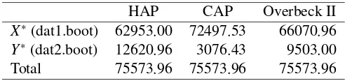
Table 4: Case I. Capital allocation based on different principles

HAP CAP Overbeck II

X∗(dat1.boot) 62953.00 72497.53 66070.96

Y∗(dat2.boot) 12620.96 3076.43 9503.00 Total 75573.96 75573.96 75573.96

5.1. Case I: Lack of dependence structure

In this subsection, we assess the performance of allocation principles we are interested in when losses exhibit a low degree of linear dependence, this means that the correlation coefficient between the losses is close enough to zero.

LetX andY be vectors consisting of 1000 and 400 observations on individual losses, moreover Public data risk no. 1 is now denoted by X and Public data

risk no. 2 is denoted byY. We will estimate risk using a Montecarlo simulation

method as follows

1. Draw 1000 observations from X and 400 from Y using re-sampling with replacement and obtainX1 andY1.

2. Generatex∗₁ =P1000

i=1 X1,iandy∗1=

P400

i=1Y1,i.

3. Repeat steps 1) and 2) 10000 times to obtain two vectors of equal lengths:

X∗_andY∗_withX∗ _={x∗

i}

10000

i=1 andY

∗_{= {y}∗ i}

10000

i=1 .

Once we have X∗ andY∗, we knowthe distribution of losses in each unit, i.e risk no. 1 and risk no. 2, respectively. We can now compute the allocations based on the principles previously discussed.

Summarizing we generate for both vectors of losses 10000 replications of size 1000 and 400 for Public data risk no. 1and for Public data risk no. 2, respec-tively in order to obtain two vectors of length 10000 over which we can apply the allocation principle we are interested in.

An aggregate capital amount of 50 416.738 _{monetary units would be enough} for facing the total loss for this particular sample comprised by X and Y (Public

data risk no. 1andPublic data risk no. 2, respectively). Nevertheless, in order to

guarantee a coverage even when large deviations might occur we use the empirical VaR99(S) = 75 573.96 that ensures 99% coverage of potential losses and this is why we set the exogenous capital to be this value. Aggregate capital to be allocated is 75 573.96 monetary units.

8

Table 4 shows the allocated capital to each vector of losses based on different capital allocation principles, these results show the amount of capital to be set aside for each risk source. Note that Haircut allocation principle (HAP) boils down to a simple proportion when there is not any dependence structure (in a linear sense) between the losses, this happens when the correlation coefficient between X∗_andY∗_{is close to zero and in this particular case such correlation is}

≈ 0.00014, therefore results obtained from HAP will be identical to those obtained using:

Ki =

K

Pn

i=1Xi

Xi, (37)

recalling the fact thatPn

i=1Xi =S, this “simple proportional” allocation principle (SPA) reduces to (K/S)Xi. When K = 1 and multiplying the result by 100 gives us the percentage ofXias a portion of the aggregate lossS as it is shown in Table 5.

According to Table 3 the losses seem to be non-normal, therefore both Haircut and Overbeck type II allocations are computed using the normal and the t-student distribution, for the t-student we used several degrees of freedom and results do not differ from those ones reported when using a normal distribution, so in Table 4 only normal results are reported.

In order to assess how well the allocations fit, we now calculate the proportions of capital to be set aside instead of the amount of capital, we reach this goal by choosingK =1 and the new results are reported in Table 5.

As it was expected, the Haircut allocation principle is a good choice since it does not take into account the dependence structure and since the correlation between X∗ and Y∗ is almost zero the best choice for this case is using (37) as the allocation principle, because its results are the a good enough approximation for HAP and its calculation is enormously simplified, furthermore it does not rely on any distributional assumption. Table 5 shows how the approximation to HAP using (37) performs compared to HAP results.

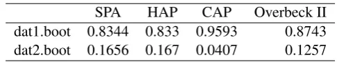
Table 5: Case I. Proportions of capital allocation based on different principles

SPA HAP CAP Overbeck II dat1.boot 0.8344 0.833 0.9593 0.8743 dat2.boot 0.1656 0.167 0.0407 0.1257

contribution of the first vector and underestimates the second one in a stronger way than Overbeck II does. In a rough sense we can see that in absence of cor-relation between losses, the estimates of the Covariance allocation principle are more biased than those of Overbeck II.

Clearly in this part of the exercise we conclude that Covariance allocation principle performs the worst compared to the other two principles.

In the next section we introduce a strong dependence structure in order to assess the performance of the allocations which account for correlation among losses.

5.2. Case II: Strong dependence structure

This section can be seen as the counterpart of the previous one as now we go to the other extreme case where a strong dependence framework is involved.

In order to create two vectors of losses strongly correlated we base the sam-pling scheme on quantiles-based extractions, this means for each probability pi with i = 1, . . . ,10000, which is common for both vectors X and Y, recall that

X is the label for Public data risk no. 1 and Y is the label for Public data risk

no. 2, we take the value located at quantile given byF_X−1(pi) andF−Y1(pi), each pi

was randomly drawn from a U(0,1), to make this point clear, we go through the following steps:

1. Draw randomly 10000 values from a U(0,1) for probabilities such that p1 is one realization ofU(0,1), p2 is another, and so on untilp10000.

2. GenerateWandZsuch that both are vectors of dimension 10000×1 holding

F−1

X (pi) and F −1

Y (pi).

3. ConstructingW andZthis way guarantees that when we have a small value for W we also have a small value for Z and when we have a large for one

W we also have a large one for Z. We store W and Z into a matrix M of dimension 10000×2 so thatW andZare now matched (pairwise).

4. Resample row-wise with replacement from Mand draw 10000 pairs of ob-servations, sum them colwise and getm1which is a 1×2 vector, repeat this step 10000 times in order to getmiwithi=1, . . . ,10000.

5. The data set we are going to work with is the matrix M∗ _{consisting of the} colwise concatenation ofmiwithi=1, . . . ,10000. M∗should look like:

M∗ =

          

m1,1 m1,2

..

. ...

m10000,1 m10000,2

          

1) andY′ is the resampled associated to the fraudulent transactions (Public

data risk no. 2). Here the apostrophe does not mean transpose, it is just a

way to nameXandY in order to distinguish them from the originalsXand

Y.

Given that we suffer from different lengths for vectors of losses, we base this part of the exercise on a resampling technique using a uniform distribution as de-scribed above, this consists of generating 10000 random numbers from a uniform distribution, U(0,1), then we use this numbers to extract the empirical quantiles from each vectors, this way we obtain two vector of length 10000 with a strong dependence structure since each time we draw a “small” value from the first vec-tor we also get a “small” value from the second one, the same happens with “big” values, this is because we are using the 10000 uniform number as index for the inverse distribution function to retrieve those numbers.

The correlation coefficient enrolled in this case is≈0.8875, this is the correla-tion between X′ _andY′_{, which is the “strong” dependence structure giving name} to this section.

Following the same idea from the previous section, we consider the total cap-ital to be allocated as exogenously determined and taken as given, so we consider this capital to be the empirical Value at Risk at 99% which is 628 724.6 monetary units.

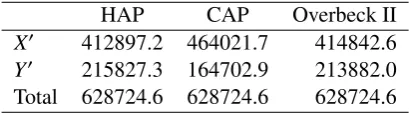
Table 6: Case II. Capital allocation based on different principles

HAP CAP Overbeck II

X′ 412897.2 464021.7 414842.6

Y′ 215827.3 164702.9 213882.0 Total 628724.6 628724.6 628724.6

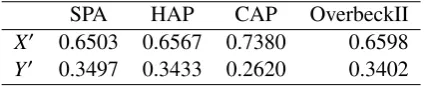
Table 7: Case II. Proportions of capital allocation based on different principles

SPA HAP CAP OverbeckII

X′ 0.6503 0.6567 0.7380 0.6598

Y′ 0.3497 0.3433 0.2620 0.3402

In terms of proportions, Table 7 gives a picture of how the principles distribute the total capital between the business units. The first column represents the results using (37), this would be the allocation if correlation between risk sources were zero, in this case the optimal distribution of the total capital should be 65.03% allocated to the first business line (bank transfer mistakes) and 34.97% to the loss caused by fraudulent transactions. Since correlation between risk sources is 0.8910, then allocation based on (37) is biased, so principles that includes the linear dependence in its calculations are needed.

In spite of the fact that HAP is based on the idea of measuring stand-alone losses using a VaR (normal VaR in this case) it performs well enough even if the correlation is high, but one has to have in mind that VaR is not a coherent risk measure so in this case it is better off using a coherent risk measure for capital allocation, from this point we can choose either Covariance allocation principle or Overbeck type II allocation principle, but in practice HAP and CAP results are not so different.

6. Conclusions and Future Research

In this study we present the allocation problem and based on [16] we provide explicit formulation for Ki when using different specifications for business unit driven principles as well as aggregate portfolio driven allocations.

The numerical exercise carried out shows that the configuration of the alloca-tions depends on the degree of linear dependence. Haircut allocation principle, even being a principle based on a non-coherent risk measure, experiences a good performance and it is less affected by the “correlation effect” (changes in the cor-relations). Haircut allocations are very similar to those suggested by Overbeck type II principle when correlation is high, this confirms the good performance of Haircut allocation principle.

[1] Abbasi, B. and Guillen, M. (2013). Bootstrap control charts in monitor-ing value at risk in insurance. EXPERT SYSTEMS WITH APPLICATIONS, 40(15):6125–6135.

[2] Ai, J., Brockett, P. L., Golden, L. L., and Guillen, M. (2013). A Robust Unsupervised Method for Fraud Rate Estimation. JOURNAL OF RISK AND

INSURANCE, 80(1):121–143.

[3] Alemany, R., Bolance, C., and Guillen, M. (2013). A nonparametric approach to calculating value-at-risk. INSURANCE MATHEMATICS& ECONOMICS, 52(2):255–262.

[4] Artis, M., Ayuso, M., and Guillen, M. (1999). Modelling different types of automobile insurance fraud behaviour in the Spanish market. INSURANCE

MATHEMATICS& ECONOMICS, 24(1-2):67–81. 1st Insurance

Mathemath-ics and EconomMathemath-ics Conference, AMSTERDAM, NETHERLANDS, AUG 25-27, 1997.

[5] Artis, M., Ayuso, M., and Guillen, M. (2002). Detection of automobile insur-ance fraud with discrete choice models and misclassified claims. JOURNAL

OF RISK AND INSURANCE, 69(3):325–340.

[6] Belles-Sampera, J., Merigo, J. M., Guillen, M., and Santolino, M. (2013). The connection between distortion risk measures and ordered weighted averaging operators. INSURANCE MATHEMATICS&ECONOMICS, 52(2):411–420.

[7] Bolance, C., Ayuso, M., and Guillen, M. (2012). A nonparametric approach to analyzing operational risk with an application to insurance fraud.JOURNAL

OF OPERATIONAL RISK, 7(1):57–75.

[8] Bolanc´e, C., Guill´en, M., Gustafsson, J., and Nielsen, J. P. (2012).

Quantita-tive Operational Risk Models. Chapman & Hall/CRC.

[9] Bolance, C., Guillen, M., Gustafsson, J., and Nielsen, J. P. (2013). Adding prior knowledge to quantitative operational risk models. JOURNAL OF

OP-ERATIONAL RISK, 8(1):17–32.

[10] Bolance, C., Guillen, M., and Nielsen, J. P. (2010). Transformation ker-nel estimation of insurance claim cost distributions. In Corazza, M and Pizzi, C, editor, MATHEMATICAL AND STATISTICAL METHODS FOR

ACTUAR-IAL SCIENCES AND FINANCE, pages 43–51. Banca Italia; Casino

Mathematical and Statistical Methods for Actuarial Sciences and Finance, Ist Veneto Sci, Lettere Arti, Venice, ITALY, MAR 26-28, 2008.

[11] Boucher, J.-P. and Guillen, M. (2011). A Semi-Nonparametric Approach to Model Panel Count Data. COMMUNICATIONS IN STATISTICS-THEORY

AND METHODS, 40(4):622–634.

[12] Buch-Kromann, T., Guillen, M., Linton, O., and Nielsen, J. P. (2011). Multivariate density estimation using dimension reducing information and tail flattening transformations. INSURANCE MATHEMATICS & ECONOMICS, 48(1):99–110.

[13] Buch-Larsen, T., Nielsen, J., Guillen, M., and Bolance, C. (2005). Ker-nel density estimation for heavy-tailed distributions using the Champernowne transformation. STATISTICS, 39(6):503–518.

[14] B¨uhlmann, H. (1970). Mathematical Methods in Risk Theory. Berling: Springer-Verlang.

[15] Caudill, S., Ayuso, M., and Guillen, M. (2005). Fraud detection using a multinomial logit model with missing information. JOURNAL OF RISK AND

INSURANCE, 72(4):539–550.

[16] Dhaene, J., Tsanakas, A., Valdez, E. A., and Vanduffel, S. (2012). Optimal Capital Allocation Principles. Journal of Risk and Insurance, 79(1):1–28.

[17] Dhaene, J., Vanduffel, S., Goovaerts, M., Kaas, R., Tang, Q., and Vyncke, D. (2006). Risk Measures and Comonotonicity: A Review. Stochastic Models, 22(4):573–606.

[18] Englund, M., Guillen, M., Gustafsson, J., Nielsen, L. H., and Nielsen, J. P. (2008). Multivariate latent risk: A credibility approach. ASTIN BULLETIN, 38(1):137–146.

[19] Furman, E. and Zitikis, R. (2008). Weighted Premium Calculation Princi-ples. Insurance: Mathematics and Economics, 42(1):459–465.

[20] Gerber, H., U. (1981). The Esscher Premium Principle: A Criticism. Com-ment. ASTIN Bulletin, 12(2):139–140.

[21] Guillen, M., Gustafsson, J., and Nielsen, J. P. (2008). Combining underre-ported internal and external data for operational risk measurement. JOURNAL

[22] Guillen, M., Maria Sarabia, J., and Prieto, F. (2013). Simple risk measure calculations for sums of positive random variables. INSURANCE

MATHE-MATICS&ECONOMICS, 53(1):273–280.

[23] Guillen, M., Nielsen, J. P., Scheike, T. H., and Maria Perez-Marin, A. (2012). Time-varying effects in the analysis of customer loyalty: A case study in insur-ance. EXPERT SYSTEMS WITH APPLICATIONS, 39(3):3551–3558.

[24] Guillen, M., Prieto, F., and Maria Sarabia, J. (2011). Modelling losses and locating the tail with the Pareto Positive Stable distribution. INSURANCE

MATHEMATICS&ECONOMICS, 49(3):454–461.

[25] Heilmann, W.-R. (1989). Decision Theoretic Foundations of Credibility Theory. Insurance: Mathematics and Economics, 8(1):77–95.

[26] Jha, S., Guillen, M., and Westland, J. C. (2012). Employing transaction aggregation strategy to detect credit card fraud. EXPERT SYSTEMS WITH

APPLICATIONS, 39(16):12650–12657.

[27] McNeil, A. J., Frey, R., and Embrechts, P. (2005). Quantitative Risk

Man-agement: Concepts, Techniques and Tools. Princeton University Press.

[28] Overbeck, L. (2000). Allocation of Economic Capital in Loan Portfolios. In

Measuring Risk in complex stochastic systems.

[29] Sarabia, J. M. and Guillen, M. (2008). Joint modelling of the total amount and the number of claims by conditionals. INSURANCE MATHEMATICS&

ECONOMICS, 43(3):466–473.

[30] Tsanakas, A. (2007). Capital Allocation with Risk Measures. InProceedings

of the 5th Actuarial and Financial Mathematics Day., pages 3–17.

[31] Tsanakas, A. (2009). To Split Or Not To Split: Capital Allocation with Convex Risk Measures. Insurance: Mathematics and Economics, 44(2):268– 277.

[32] Viaene, S., Ayuso, M., Guillen, M., Van Gheel, D., and Dedene, G. (2007). Strategies for detecting fraudulent claims in the automobile insurance industry.

EUROPEAN JOURNAL OF OPERATIONAL RESEARCH, 176(1):565–583.

AND TELECOMMUNICATIONS, volume 3275 of LECTURE NOTES IN

COMPUTER SCIENCE, pages 78–87. Inst Comp Vis & Appl Comp Sci. 4th

Industrial Conference on Data Mining (ICDM), Leipzig, GERMANY, JUL 04-07, 2004.