Munich Personal RePEc Archive
Taxing Pollution: Agglomeration and
Welfare Consequences
Berliant, Marcus and Peng, Shin-Kun and Wang, Ping
Washington University in St. Louis, Academia Sinica, National
Taiwan University
25 March 2013
Online at
https://mpra.ub.uni-muenchen.de/45520/
Taxing Pollution: Agglomeration and Welfare Consequences
Marcus Berliant, Washington University in St. Louis Shin-Kun Peng, Academia Sinica and National Taiwan University
Ping Wang, Washington University in St. Louis and NBER March 2013
Abstract: This paper demonstrates that a pollution tax with a …xed cost component may lead, by itself, to strati…cation between clean and dirty …rms without heterogeneous preferences or increasing returns. We construct a simple model with two locations and two industries (clean and dirty) where pollution is a by-product of dirty good manufacturing. Under proper assumptions, a completely strati…ed con…guration with all dirty …rms clustering in one city emerges as the only equilibrium outcome when there is a …xed cost component of the pollution tax. Moreover, a strati…ed Pareto optimum can never be supported by a competitive spatial equilibrium with a linear pollution tax that encompasses Pigouvian taxation as a special case. To support such a strati…ed Pareto optimum, however, an e¤ective but unconventional policy prescription is to redistribute the pollution tax revenue from the dirty to the clean city residents.
JEL Classi…cation: D62, H23, R13.
Keywords: Pollution Tax, Agglomeration of Polluting Producers, Endogenous Strati…cation.
Acknowledgments: We are grateful for suggestions from an anonymous referee, Sören Blomquist, John Conley, Katherine Cu¤, Hideo Konishi, Ailsa Röell, Steve Slutsky, John Weymark, and Jay Wilson, as well as participants at the Public Economic Theory Conference in Taipei, the Regional Science Association International Meetings in Miami, and the Taxation Theory Conference at Van-derbilt University. Financial support from Academia Sinica and the National Science Council of Taiwan (grant no. NSC99-2410-H-001-013-MY3) that enabled this international collaboration by the Three Mouseketeers is gratefully acknowledged. Needless to say, the usual disclaimer applies.
“If you visit American city, You will …nd it very pretty.
Just two things of which you must beware: Don’t drink the water and don’t breathe the air.” (Tom Lehrer, Pollution)
1
Introduction
It is evident that the development of many local economies has featured adjacent but separate
clean and dirty cities. Examples of such pairs include Seattle/Tacoma and San Francisco/Oakland
with larger clean cities, Ann Arbor/Detroit and Aurora/Denver with smaller clean cities, as well
as Washington, D.C./Baltimore with comparably sized clean and dirty cities. A natural question
arises: Why are dirty …rms clustered in one location and why is such an outcome sustainable
over time? Certainly one might address the question with heterogeneity in preferences or increasing
returns in production, for example internal increasing returns of the type used in the New Economic
Geography literature; see the recent paper by Picard and Tabuchi (2010) and papers cited therein.1
Our paper proposes an alternative: a pollution tax with a …xed cost tax component may, by itself,
lead to strati…cation between clean and dirty …rms without heterogeneous preferences or increasing
returns.
Since 1972, the OECD has adopted the polluter pays principle, trying to internalize
environ-mental costs based on the idea …rst advanced by Pigou (1920). More recently, the OECD (1994)
categorized three types of pollution taxes: (i) a proportional tax on the actual pollution output,
for example according to the amount of emission; (ii) a proportional tax on a proxy for pollution
output, for example according to water consumption, electricity usage or each unit of product when
the production process harms the environment; and (iii) a …xed cost tax levied on each company
or each household. In this paper, we consider all three types. Whereas a …xed cost tax levied on
each …rm is considered, the proportional Pigouvian tax is generalized to a linear tax that includes
a …xed cost tax component as proposed by Carlton and Loury (1980).2
1See Porter (1990) for a comprehensive discussion of industrial clustering from a business strategy viewpoint. Our
paper is also related to the locational strati…cation literature, where strati…cation is caused by human capital (cf. Benabou 1996a,b, Chen, Peng and Wang 2009), local public goods (cf. Nachyba 1997 and Peng and Wang 2005), and the environment (cf. Chen, Huang and Wang 2012).
2See also Baumol (1972) and Buchanan and Tullock (1975) on direct control versus taxation, and Chipman and
In brief, the purpose of this paper is as follows. We construct a simple model with two locations
and two industries (clean and dirty) where pollution is a by-product of dirty good manufacturing,
and dirty good manufacturing is subject to agglomeration externalities with decreasing private
returns to scale. We could obtain our results without agglomeration externalities, but they help
simplify the analysis and calculations, as we shall explain below. Next, we establish conditions under
which a completely strati…ed con…guration with all dirty …rms clustering in one city emerges as the
only equilibrium outcome when there is a …xed cost component of the pollution tax. Finally, we
show that a strati…ed Pareto optimum can never be supported by a competitive spatial equilibrium
under a linear pollution tax without redistributing the pollution tax revenue from the dirty to the
clean city residents.
Regarding our examples of pairs of clean and dirty cities in the US, it is important to point out
from where, in our view, the …xed component of a pollution tax arises. As discussed by Karp (2005,
pp. 229-230), if …rms pay a unit tax based on the aggregate level of pollution, in technical terms an
“ambient tax,” but if they think that they are so small that they have no e¤ect on the aggregate
level of pollution, then they view the tax as a …xed cost.3 Of course, such an ambient tax may
vary by location, as aggregate pollution is generally location-speci…c. Such a tax is essentially an
aggregate amount of required revenue (the tax rate multiplied by total pollution) divided up among
…rms in the local polluting industry, which is exactly the way we model it.4
Our main result establishes that taxing pollution with a …xed component independent of dirty
good output can cause …rm agglomeration (a variable tax component on top of the …xed component is
permitted). The key argument is as follows. At a symmetric, integrated equilibrium, wages equalize
both across sectors and locations. Then, in the presence of a …xed total pollution damage payment in
each polluted region, dirty factories may not have su¢cient pro…tability to pay the tax and thus no
integrated equilibrium exists. Now if dirty …rms cluster, as they do in a strati…ed equilibrium, then
they share the …xed pollution tax in the one region where they cluster, implying higher net of tax
pro…t. Moreover, wage equalization between the two locations is no longer required in equilibrium
because clean and dirty …rms are in two di¤erent locations, so there is no wage equalization even
taxation for production agglomeration, in particular when pollution is local (so location is relevant) and agents are mobile. The point of Carlton and Loury (1980) is di¤erent, in that they are concerned with …rm entry and exit. We do not consider that in our model.
3Karp (2005) goes on to consider the case where …rms are large so each has an e¤ect on the aggregate level of
pollution.
4A natural alternative model, that does not capture this idea, is to use a …xed lump-sum tax for each …rm entering
across sectors. All we need is utility equalization, which only requires that pollution disutility
balance with the wage di¤erential. This is consistent with …rm pro…tability under strati…cation.
The important part of the argument is as follows. Both the …xed component of the pollution tax
and decreasing private returns are needed for this result, as indicated above. The …xed component
of the pollution tax rules out integrated equilibrium. With decreasing private returns that permit
positive rent for dirty …rms, agglomeration ensures enough pro…tability of dirty …rms when fully
clustered to allow existence of strati…ed equilibrium with the tax. There is a positive feedback
loop: With a variable tax component, more pollution in a region implies more tax revenue that
attracts more worker/consumers (who receive the revenue), thus depressing the wage. A potential
o¤setting factor is that the wage must be higher in the region to compensate for disutility due to
more pollution. In the end, the equilibrium con…guration is a function of the parameters.
The key di¤erence between this work and the classical literature on Pigouvian taxation is: We
assume that there is a local government in each region that must balance its own budget. We take
the tax system of each local government to be exogenous and uniform, with no tax competition.5
The taxes could be set by a higher level of government. But the revenues stay local. For example,
the tax revenues could pass through a higher level of government and be returned to the local
government in some form such as funding for a local public good. In other words, we are making
an important distinction between the authority that sets the tax on pollution, and the recipients of
the revenue.
There are 3 related potential distortions in our framework: a negative pollution externality
from dirty …rm production imposed on consumers, a positive local agglomeration externality for
polluting …rms, and a migration incentive for consumers induced by the tax and redistribution
schedules in the two regions. Regarding the last distortion, local tax revenue and local pro…ts are
distributed back to the residents of that location only. The setting would be classical if there were
only one national government with the power to tax di¤erentially and redistribute to consumers
independent of region of residence. In that case, the standard welfare theorems would go through
under Pigouvian taxes, since correction for the pollution externality and migration incentives (the
…rst and third distortions) can be made in the usual way, whereas the …xed cost component of the
…rm tax/transfer system can account for the agglomeration externality. However, with independent
regional government taxation as in our setting, equilibrium allocations might not be Pareto optimal
unless transfers between the regional governments are made so that the regional governments can
5The reader is referred to Markusen, Morey, and Oleviler (1995) for modeling …scal competition in pollution taxes
mimic a national government.
Turning next to a detailed description of our model, to illustrate the possibility that a pollution
tax causes agglomeration of dirty …rms, we construct a simple model featuring two industries, clean
and dirty. Both industries use homogeneous labor as inputs. Whereas the clean service production
is Ricardian (constant returns), dirty manufactured good production is socially
constant-returns-to-scale and privately diminishing returns with positive spillovers of the Romer type. Pollution is a
by-product of dirty good manufacturing. To eliminate unnecessary complications associated with a
wealth e¤ect, utility is assumed to be quasi-linear, linear in clean good consumption and pollution
but strictly increasing and strictly concave in dirty good consumption. The pollution tax schedule
features a …xed cost tax component that is independent of pollution (or dirty good output) and
may also contain a marginal tax component that is proportional to dirty good output.
We establish that under proper assumptions, a completely strati…ed equilibrium with all dirty
…rms clustered in one city is supported and such a strati…ed equilibrium cannot emerge in the
absence of the …xed payment pollution tax. In some circumstances, an integrated equilibrium is
impossible, but a strati…ed equilibrium exists. Under suitable conditions, we show thatthe presence
of pollution and a pollution tax with a …xed cost tax component, rather than the Romer-type positive
spillovers, are necessary for agglomeration of dirty …rms. Our main …ndings are robust, and remain
valid even when: (i) quasi-linearity of utility is abandoned, or (ii) allowing producers to choose
between clean and dirty good technologies. We have assumptions on the model’s reduced form that
will generate either integrated or strati…ed equilibrium. We do not push them back to primitives,
as there are many exogenous parameters and thus many combinations that will work for each type
of con…guration. However, in Remarks 6 and 7 below, we …x all but 2 parameters and provide a
description of parameter ranges where the respective equilibrium con…gurations arise.
Next we turn to the examination of Pareto optima. Depending on exogenous parameter values,
both integrated and strati…ed con…gurations can arise as optima. Whereas an integrated Pareto
optimum can be supported by a competitive spatial equilibrium with a linear pollution tax, a
strati…ed Pareto optimum cannot. Speci…cally, regardless of the linear pollution tax schedule, a
strati…ed equilibrium is always over-polluted compared to the optimum. To support the strati…ed
Pareto optimum, one must redistribute pollution tax revenues from the dirty to the clean city
residents. This suggests a new instrument to rectify competitive equilibrium ine¢ciency when there
is pollution generated by dirty good production.6
6We wish to emphasize that in this paper, we consider only equilibrium or optimal con…gurations that are completely
The remainder of the paper is organized as follows. Section 2 contains the notation and basic
model. Section 3 provides …rst order necessary conditions for equilibrium. Section 4 analyzes the
two types of equilibria we consider here, namely integrated and strati…ed. Section 5 analyzes the
conditions on parameters that generate each of these types of equilibria. Section 6 gives further
results, particularly about stability of equilibrium, that can be derived with speci…c functional
forms, namely an example. Section 7 discusses Pareto optima and the welfare theorems, whereas
section 8 concludes.
2
The Model
Consider a local economy consisting of two regions/cities (i=A; B) and two sectors (a clean/service
goodX and a dirty/manufactured goodY). Each region has an abundant supply of land of density
one in a featureless landscape. Land is omitted from the benchmark model for tractability reasons,
so the model looks more like one of coalition formation than of an urban economy. Goods are freely
mobile and there is no cost to transport any commodity between regions. Throughout the paper,
the clean good is taken as the numéraire.
This local economy is populated with three groups of active agents: (i) a continuum of households
of a …xed mass one, who are all both consumers and workers; (ii) a continuum of clean
(non-polluting) …rms of mass one, and (iii) a continuum of dirty ((non-polluting) …rms of mass M > 0. All
households arefreely mobile between the two regions, but once a household has chosen a residential
location, it cannot commute between the two regions. This latter assumption is equivalent to
assuming that the commuting cost between two regions is su¢ciently high. Such an assumption is
justi…able when the two regions are su¢ciently far apart: for many clean-dirty city pairs in the real
world such as Ann Arbor-Detroit and Seattle-Tacoma, the fraction of people commuting between
cities is essentially negligible. We will discuss in Section 5.1 (see Remark 4) what happens if workers
are allowed to commute between the two regions.
In addition to the three groups of active agents, there is a local government ruling each region,
whose only activity is to collect pollution taxes/fees for redistribution to consumers. To close the
economy, we shall assume that dirty …rms in a particular region are owned by consumers in the
same region.
2.1 Firms
The clean good is produced with labor input under a Ricardian technology,
xi(j) = nix(j); i=A; B; j2[0; ki] (1)
where xi(j) denotes the output of clean …rm j in location i, > 0 is the inverse of the unit
labor requirement for clean good production,nix(j) represents clean …rmj’s demand for labor, and
ki 2 [0;1]denotes the mass of clean …rms in region i. The total local supply of the clean good in
region i is given by Xi =
Z ki
0
xi(j)dj and the total local clean industry employees in the region i
can be speci…ed as:
Nxi =
Z ki
0
nix(j)dj i2A; B (2)
Underex post symmetry of …rms in a region, imposed throughout, we have Nxi =kinix.
Denote by mi the mass of dirty …rms in region i, byniy(j) the labor demand by a dirty …rm j
in regioni, and byNyi the total local dirty industry employees in regioni, where:
Nyi =
Z mi
0
niy(j)dj i2A; B (3)
Each dirty good …rm employs labor as the sole private input under a privately
decreasing-returns-to-scale and socially constant-returns-decreasing-returns-to-scale production technology fe:
yi(j) =f ne iy(j); Nyi =Nyif n
i y(j)
Ni y
!
; i2A; B; j2[0; mi] (4)
where yi(j) is the output of dirty …rm j in region i. We assume that feis strictly increasing and
strictly concave in each argument, satisfying the boundary condition fe 0; Nyi = 0 and the Inada
conditions limni y(j)!0
@fe(ni y(j);Nyi)
@ni
y(j) = 1 and limn i y(j)!1
@fe(ni y(j);Nyi)
@ni
y(j) = 0. Under social constant
returns, we can divide …rm output by the total number of local dirty industry employees to obtain
f, where the properties offeimply that f is strictly increasing and strictly concave in the fraction
of …rm employees in the local dirty industry. The incorporation ofNyi into a dirty …rm’s production
function captures positive spillovers of the Romer (1986) type, where Nyi is a positive measure of
small …rms, and where each …rm is of measure zero. Under an ex post symmetric equilibrium,
Ni
y =miniy. The presence of uncompensated positive externalities provides an agglomeration force for dirty …rms. Nonetheless, we will show in Sections 5.1 and 6.1 that the presence of pollution and
a pollution tax with a …xed cost tax component, rather than the Romer-type positive spillovers, are
Both goods (clean and dirty) are traded and freely mobile. Letpdenote the global relative price
of the dirty good. Further denote the wage rate prevailing in regioniaswi. Let the region-speci…c
pollution tax in regionibe i (to be speci…ed later), where pi represents a typicalad valorem tax.7
Each dirty …rm in region ichooses labor demand to maximize its pro…t; its optimization problem
is then given by:
i(j) = max ni
y
p
"
Nyif n
i y
Ni y
! i
#
winiy(j) (5)
The aggregate output of the dirty good in regioniisYi = Z mi
0
yi(j)dj.
2.2 Households
Each household values the consumption of the clean good and the dirty good but su¤ers disutility
from pollution. Each household is endowed with one unit of labor. Since a household does not value
leisure, the entire one unit of labor is supplied inelastically. LetQi measure the level of pollution in
regioni. Following conventional wisdom, we assume that pollution is a by-product of the production
of dirty goods, taking a simple linear form:
Qi = Yi =
Z mi
0
yi(j)dj (6)
where >0. The utility of a household residing in region itakes a quasi-linear form:
Ui =cix Qi+u(ciy) (7)
This utility function is quasi-linear in the spirit of Bergstrom and Cornes (1983): linear in clean
good consumption cx and total pollution Q, but nonlinear in cy, as u(cy) is the utility obtained
from consuming the dirty good. It is strictly increasing and strictly concave, satisfying the boundary
condition u(0) = 0and the Inada conditionslimci y!0u
0
(ciy) =1and limci y!1u
0
(ciy) = 0.
The household’s budget constraint in region iis simply speci…ed as follows:
cix+pciy =wi+zi (8)
where zi represents the sum of government rebates (of pollution tax collection) and …rm pro…t
redistribution in regioni:
zi= 1
Ni Z mi
0
i(j) +p i dj; i2A; B (9)
Quasi-linear preferences imply that, by substituting in the budget constraint (8), household’s
utility can be rewritten as:
Ui= wi+zi Qi+ u(ciy) pciy
which is income net of pollution disutility plus the consumer surplus derived from consuming the
dirty good. Thus, household’s optimization reduces to one variable: maximization of the consumer
surplus from dirty good consumption, which simpli…es the analysis greatly. We will discuss in
Section 5.1 (see Remark 3) what happens if the utility of the clean good is strictly concave.
2.3 The Local Government
The pollution tax levies on the dirty …rm are given as follows:
i = 8 <
:
0; ifyi(j) = 0;8 j
gi(yi(j); Yi); otherwise
When pollution is nondegenerate, we shall consider two speci…c regimes of interest, namely, a …xed
pollution tax regime and a linear pollution tax regime:8
gi =
8 <
:
F=mi, under …xed pollution tax regime
L+tyi(j), under linear pollution tax regime
Under the …xed pollution tax regime, a …xed levy F > 0 is imposed on region i so that each
…rm pays an equal share mFi; under the linear pollution tax regime, in addition to a lump-sum
tax L > 0, a marginal tax t > 0 is imposed on …rm output yi. Whereas the former can best
illustrate the role of pollution taxation played in …rm agglomeration, the latter is important because
it encompasses Pigouvian taxation as a special case and allows practical welfare analysis. For
notational convenience, we shall denote generally the marginal tax rate as:
@ i @yi(j) =
8 <
:
0, under …xed pollution tax regime
t, under linear pollution tax regime
3
Optimization and Equilibrium
We are now prepared to derive individual optimizing conditions and to specify market clearing
conditions.
8This functional form also covers the …rst type of tax mentioned in the introduction because pollution is proportional
3.1 Optimization
The …rst-order condition for pro…t maximization of each clean and dirty …rm is, respectively, given
by:
=wi (10)
V M PL p(1 )M P Liy =p(1 )f
0 n
i y
Ni y
!
=wi (11)
where V M PL denotes the value of the marginal product of labor (or marginal revenue product)
and M P L denotes the marginal product of labor. Denote the dirty …rm’s surplus accrued from
uncompensated spillovers as:
(e) f(e) (1 )ef0
(e)
where e niy
Ni
y. It is convenient to denote the dirty …rm’s surplus excluding pollution tax as
e(e) = f(e) ef0
(e): Given our assumptions on the production function for dirty …rms, both
(e)and e(e) are strictly increasing ine. Substituting theex post symmetry condition,Nyi =miniy
as well as (11) and (3) into (5) yields the pro…t for every …rmj in regioni:
i(j) = i =p ni
ymi 1=mi i (12)
The lump-sum distribution to each household follows immediately:
zi = (m
i)2
Ni 1=m i pni
y,8 i (13)
The household’s optimization problem can be written more simply in two steps, solving backward.
In the second step, households choose their best consumption bundle subject to their budget in each
region. In the …rst step, they choose their region of residence.
Beginning with the second step, each household residing in region i maximizes their utility
subject to the budget constraint by choosingciy:
max
ci y
wi+zi pciy Qi+u ciy (14)
The …rst-order condition of (14) with respect tociy is given by:
u0
ciy =p (15)
It is immediate that, since the relative price of the dirty good across the two regions is one, the
consumption of the dirty good in the two regions must be identical too. From the budget constraint
(8) and (15), we then solve the clean good consumption as:
cix =wi+zi pcyi =wi+zi ciyu0
Substituting (11), (13), and (15) into (16), we have the consumption of the clean good in region i
as:
cix=u0
ciy (1 )f0
1=mi +(m
i)2
Ni 1=m i ni
y ciy (17)
In the …rst step, the household’s residential location can be determined by:
i= arg max
i U
i (18)
3.2 Market Clearance
Denote region i’s labor supply as Ni and recall that total labor supply is normalized to one (the
total measure of consumers). The regional and overall labor market clearing conditions are thus:
Nxi +Nyi = Ni (19)
NA+NB = 1 (20)
Moreover, goods market clearing conditions are: X
i=A;B
Nicix= X
i=A;B Z ki
0
xi(j)dj =XA+XB (21)
X
i=A;B
Niciy = X
i=A;B Z mi
0
yi(j)dj =YA+YB (22)
By symmetry, we have:
X
i=A;B
Nicix = X
i=A;B
kixi=XA+XB (23)
X
i=A;B
Niciy = X
i=A;B
miyi =YA+YB (24)
wheremA+mB =M.
Finally, if both locations are occupied, locational equilibrium requires:
UA=UB (25)
4
Equilibrium Con…guration
Acompetitive spatial equilibriumis a tuple of quantities,fni
x(j); niy(j); Nxi; Nyi; Ni; ki; mi; cix; ciy; xi(j);
yi(j); Qig, and prices, fwi; pg, such that: (i) all households and …rms optimize; (ii) labor markets
clear; (iii) goods markets clear; (iv) the population identity holds; and (v) the locational equilibrium
condition is met.9 Among all possible equilibrium con…gurations, we are particularly interested in
9The equilibrium concept is based on the multi-class equilibrium concept constructed by Hartwick, Schweizer and
two equilibria: The …rst type is anintegrated equilibrium where all clean and dirty …rms are spread
symmetrically over the two regions so that both types of …rms are completely integrated
location-ally. The second type is astrati…ed equilibrium where all dirty manufacturing …rms agglomerate in
one region (without loss of generality, let it be region A) and all clean service …rms are located in
region B (where workers face better environmental conditions). In order to compare the
endoge-nous variables obtained under the two types of equilibria, we shall use argumentsI andS to denote
integrated and strati…ed patterns, respectively.
4.1 Case I: Integrated Equilibrium
In an integrated equilibrium, both …rms and households are symmetrically distributed across the
two regions. Thus, we have:
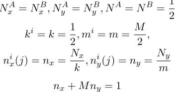
NxA=NxB; NyA=NyB; NA=NB= 1 2
ki =k= 1 2; m
i =m= M
2 ;
nix(j) =nx =
Nx
k ; n
i
y(j) =ny =
Ny
m
nx+M ny = 1
Moreover, wages must be equalized between the clean and the dirty sectors in each region. From
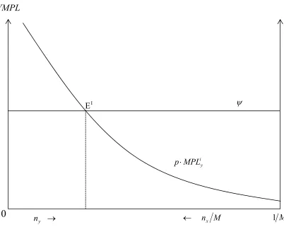
(10) and (11), we can thus depict in Figure 1 the labor allocation between clean and dirty sectors
under the integrated equilibrium.
[image:13.612.228.404.302.395.2][Insert Figure 1 here]
Figure 1 illustrates that dirty …rms’ labor demand, which is a downward-sloping function ofni y=Nyi, is determined by wage equalization between the clean and the dirty sectors (see point EI), namely
where:
p(1 )M P Ly =p(1 )f0(2=M) =w= (26)
which determines the relative price of the dirty good as a decreasing function of the mass of dirty
…rms. The Inada conditions assumed are su¢cient for the existence of an interior level of dirty
industry employment and production.
Under symmetry, a dirty …rm’s output is now given by, y = f 1=mi mini
y = M2 f(2=M)ny.
From the dirty good market clearing condition,ci
y =cy =M y, so we have:
cy =M y=
M2
This dirty good market clearing condition enables us to express the dirty good demand as a linear,
upward-sloping function of the induced demand for labor starting from the origin, which is referred
to as thedirty good market-clearing (DM) locus (see Figure 2). Moreover, we can combine (26) and
(15), yielding thedirty good optimization (DO) locus:
u0
(cy) =
(1 )f0(2=M) (28)
Thus, the demand for the dirty good is independent of the induced demand for labor.
[Insert Figure 2 here]
As depicted in Figure 2, one can see that the integrated equilibrium quantity of the dirty good and
employment are jointly determined at point EI.
Clean good market clearance implies:
cx=x= nx(I) = [1 M ny(I)]
One may easily check that one of (8), (27) and the above equation are redundant, i.e., Walras’ law
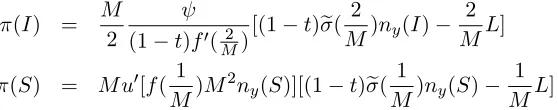
is veri…ed. Substituting the equilibriumny(I) and (28) into (12), we have:
(I) = M
2 (1 )f0(2=M) (2=M)ny(I) (2=M)
i (29)
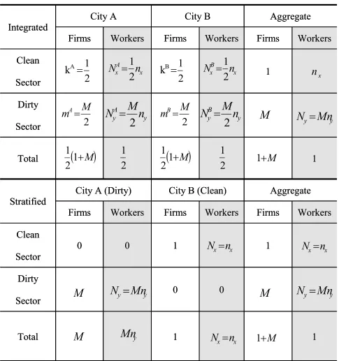
Finally, locational equilibrium (25) in this case is trivial. See Table 1 for a summary of the values
of the endogenous variables at equilibrium.
4.2 Case II: Strati…ed Equilibrium
Now, we move to examine strati…ed equilibrium. At a strati…ed equilibrium, assume that the
dirty …rms agglomerate in regionA, and the clean …rms agglomerate in region B. Then strati…ed
equilibrium is as shown in Table 1, and we have:
kA= 0; kB= 1; mA=M; mB= 0; B =zB = 0
NA=M ny; NB=nx; nx+M ny = 1
Thus, we obtain the dirty good production for each dirty …rm in regionA as: y=f m1A mAnAy =
M f(1=M)ny. In this case, wages need not be equalized between the two regions: those residing in
two regions are equal. The wages in the regionsAand B arewA=p(1 )f0
(1=M)and wB = ,
respectively. The dirty good market clearing condition implies:
cy =M y=M2f(1=M)ny (30)
which can be combined with (15) to yield:
p=u0
M2f(1=M)ny (31)
By diminishing marginal utility, the above expression entails a negative relationship between dirty
good price and employment (see the bottom panel of Figure 3). From the clean good market clearing
condition, one obtains: NAcA
x +NBcBx =x= nx, or, using (8) and Table 1,
cx(S) =x= nx= (1 M ny)
which can again be used with (8) and (30) to verify Walras’ law.
Next, we can rewrite (12) under strati…ed equilibrium as:
(S) =M u0
f(1=M)M2ny(S) (1=M)ny(S) (1=M) i (32)
The equilibrium level of pollution in regionAis given by: QA= YA= M y= M2f(1=M)ny(S). We can derive the utility level attained by households residing in regionA as:
UA=M f(1=M) u0
f(1=M)M2ny(S) [1 M ny(S)] M ny(S) +u f(1=M)M2ny(S)
Since there are no dirty …rms and thus no pollution in regionB, in equilibrium there is no pollution
tax revenue nor redistribution of dirty …rm pro…ts in region B. The utility level attained by a
household residing in regionB is:
UB = f(1=M)M2ny(S)u0 f(1=M)M2ny(S) +u f(1=M)M2ny(S)
We can then compute the utility di¤erence between regions Aand B as:
U UA UB=M f(1=M) u0
f(1=M)M2ny(S) M ny(S) (33)
By employing (31) and (33), we determine the strati…ed equilibrium relative price p and dirty
…rm labor demandny(S) as shown in Figure 3. Speci…cally, from the top panel of Figure 3, utility
equalization pins down the equilibrium level of dirty industry employment under strati…cation,
which can be plugged into the bottom panel to obtain the relative price of the dirty good.
5
Characterization of Equilibrium
Before turning to each of the two speci…c pollution tax regimes, one may compare dirty sector
employment per …rm,ny(I) and ny(S), under integrated and strati…ed equilibrium, respectively.
In an integrated equilibrium, we can use the dirty good market clearing condition and the dirty
good demand, (27) and (28), to derive:
u0 M2
2 f(2=M)ny = (1 )f0(2=M) (34)
In a strati…ed equilibrium, we can apply the location equilibrium condition in (33) to obtain:
(ny) u0 M2f(1=M)ny M ny =
M f(1=M) (35)
where (ny)measures the household’s net surplus from consuming the dirty good.
These equilibrium relationships can be referred to as thedirty good market equilibriumloci, DE(I)
and DE(S), respectively, under integrated and strati…ed con…gurations (see Figure 4). Whereas the
DE(I) locus yields the equilibrium ny(I) as shown in the top panel of Figure 4, the DE(S) locus
pins down the equilibrium ny(S) as depicted in the bottom panel of Figure 4. In the top panel of
Figure 4, the LHS of DE(I) yields a downward sloping locus as a result of diminishing marginal
utility, whereas the RHS is simply a constant that is decreasing in the exogenous mass of dirty
…rms. Thus, the integrated equilibrium is pinned down at pointEI. In the bottom panel, the LHS
of DE(S), (ny), is also a downward sloping locus and the RHS a constant depending negatively
on the exogenous mass of dirty …rms. These loci determine the strati…ed equilibrium at point ES.
To establish nice su¢cient conditions for strati…cation in the next two subsections, we shall restrict
our attention to a plausible scenario with ny(I) < ny(S), i.e., dirty industry employment under
integration is lower than that under strati…cation. It is clear from the de…nition of (ny) that the
above scenario is more likely to arise the smaller is. In other words, for all of the results below,
we shall assume that is small, a condition su¢cient to ensure that dirty industry employment
under integration is smaller than under strati…cation.
[Insert Figure 4 here]
5.1 Fixed Pollution Tax Regime
We examine under what conditions the strati…ed equilibrium emerges under the …xed pollution
government under the two di¤erent con…gurations is given by:
i= 8 < :
2F=M; for CaseI
F=M; for CaseS
For purposes of comparison, in the strati…ed case only one local government raises pollution tax
revenue, whereas in the integrated case each local government raises the same revenue as the dirty
city in the strati…ed case. One interpretation of this assumption is that the simple presence of
pollution in a city is enough to trigger a tax.
We impose a regularity condition on the dirty …rm’s surplus from uncompensated spillovers:
Condition R-1: (Regularity Condition on a Dirty Firm’s Surplus)
1
4e(2=M)<e(1=M)
Under Condition R-1, we then consider the following:
Condition S-1: (Su¢cient Condition for Strati…cation Under a Fixed Tax)
1
4e(2=M)<
F M2n
y(S)
<e(1=M)
We can then establish:
Theorem 1: (Strati…ed Equilibrium) Consider a local economy in which pollution production
is not too severe and pollution disutility is not too high, in other words is su¢ciently small.
Under Condition R-1, we suppose that the …xed pollution tax is moderate so that the inequalities in
Condition S-1 are met. Then the strati…ed con…guration arises as an equilibrium outcome, but the
integrated con…guration does not.
Proof. The proofs of all the theorems and propositions are relegated to the Appendix.
Thus, under Condition R-1, Condition S-1 is su¢cient to ensure that the strati…ed con…guration is
an equilibrium outcome, but the integrated con…guration is not. Intuitively, the …rst inequality of
Condition S-1 implies negative pro…t received by dirty …rms under integration, whereas the second
inequality guarantees positive pro…t obtained by dirty …rms under strati…cation. The main tipping
point here is the gains from clustering under the …xed pollution tax regime.
Remark 1: (Impossibility of Integrated Equilibrium) It is not di¢cult to show that when F is
Remark 2: (On the Role of Agglomerative Externalities) It is important to note that despite
the agglomeration force from uncompensated spillovers, the key driving force for all dirty …rms to
cluster in one region (A) is the presence of a …xed pollution tax that is independent of an individual
…rm’s output. Speci…cally, with F = 0, it is clear that (I) > 0, implying that the integrated
con…guration always arises in equilibrium. Moreover, we can compute the pro…ts under the two
con…gurations as follows:
(I) = M
2 f0(2=M)e(2=M)ny(I)
(S) = M u0
M2f(1=M)ny(S) e(1=M)ny(S)
Further, assume that 12e(2=M) > e(1=M). Then, dirty …rms will incur higher pro…t under inte-grated equilibrium compared to strati…ed equilibrium when the following inequality is met:
1
2e(2=M)
e(1=M) >
u0
M2f(1=M)n
y(S) ny(S)
f0(2=M)ny(I)
Refer to the top panel of Figure 4. The ratio on the right-hand side of the above inequality is
measured by the ratio of the lightly shaded area covering EO to the shaded area coveringEI. As
long as this ratio is less than 12e(2=M)
e(1=M) (which is greater than one under the additional condition
stated above), dirty …rms will earn higher pro…ts under an integrated equilibrium compared to a
strati…ed equilibrium, and thus is viable whenever the strati…ed equilibrium is viable.
An important, related point is that we could accomplish our goal without any agglomeration
externalities at all. Suppose that we simply used a decreasing returns technology for dirty …rms,
so that they make positive pro…ts in any equilibrium without taxes. With the tax as speci…ed,
for F low both integrated and strati…ed equilibria will exist, with pro…ts higher under strati…ed
equilibrium. For higher F, only strati…ed equilibrium exists, as dirty …rm pro…ts are negative at
integrated equilibrium. But this argument neglects an important issue. In comparing the integrated
and strati…ed equilibria, there is movement along the supply curve for the dirty good due to wage
di¤erences (for the compensating di¤erential from pollution), resulting in price changes and thus
demand changes for the consumption goods as well. So the comparison is not that easy. Allowing for
agglomeration externalities with socially constant returns actually simpli…es the analysis because the
dirty good production function (inclusive of the agglomeration externality) is linear in equilibrium.
Nonetheless, once we have speci…c functional forms for the dirty good production technology, we
will be able to return to this issue and provide a more concrete discussion (see Remark 7 in Section
Remark 3: (On Strictly Concave Utility of the Clean Good) Suppose the utility of the clean
good is strictly concave but the clean good (say, food) is more of a necessity than the dirty good
in the sense that the income elasticity of demand for the clean good is lower than that of the
dirty good. (In the current speci…cation, the income elasticity of the demand for clean good is, by
construction, one.) Then, for a richer jurisdiction, the willingness to pay for the pollution-generating
good is higher, making integration more likely to survive the equilibrium pro…tability test. That
is, consideration of a more general utility function speci…cation with the clean good being more of
a necessity than the dirty good reduces the likelihood of dirty …rms clustering. Thus, the presence
of income e¤ectsper se isnot as important as therelative income elasticity of demand for the two
consumption commodities.
Remark 4: (On Interregional Commuting of Workers) Recall that, in our benchmark model, at
any strati…ed equilibrium, utility levels, but not wages, are equated between cities. What happens
if commuting between cities is allowed? Notice that in our model all households have identical
utility functions. Suppose we go to another extreme, setting commuting cost to zero. Free
com-muting implies that wage equalization also holds even under strati…cation. This wage equalization
condition restricts the dirty …rm’s pro…tability, making strati…cation less likely to emerge as an
equilibrium outcome. In conclusion,su¢ciently high intercity commuting cost is necessary for dirty
…rm clustering to arise in equilibrium.
5.2 Linear Pollution Tax Regime
Under the linear pollution tax regime, =tand
g=
8 <
:
L+ tM2 f(M2 )ny(I), in integrated equilibrium
L+tM f(M1 )ny(S), for strati…ed equilibrium
We impose a stronger regularity condition on the dirty …rm’s surplus from uncompensated spillovers:
Condition R-2: (Regularity Condition on a Dirty Firm’s Surplus)
1
2e(2=M)<e(1=M)
Under Condition R-2, we further consider the following condition:
Condition S-2: (Su¢cient Condition for Strati…cation Under Linear Tax)
1
2e(2=M)<
L
(1 t)M ny(S)
This ensures:
Theorem 2: (Strati…ed Equilibrium) Consider a local economy in which pollution production is
not too severe and pollution disutility is not too high, in other words is su¢ciently small. Under
Condition R-2, we suppose that the lump-sum component of the linear pollution tax is moderate and
the marginal tax rate is not too high so that the inequalities in Condition S-2 are met. Then the
strati…ed con…guration arises as an equilibrium outcome but the integrated con…guration does not.
In Section 6 below, we shall verify that both the presence of pollution and the presence of a
…xed tax are crucial for a stable strati…ed equilibrium to arise.
6
The Case with Speci…c Functional Forms
Under the …xed pollution tax regime, we are left to check whether the strati…ed equilibrium is
stable. Due to the di¢culty of examining stability in the general setting, we shall conduct our
analysis under speci…c functional forms for the dirty good production technology and the subutility
for the dirty good. Speci…cally, we assume thatfeand u both take simple Cobb-Douglas forms:
e
f niy(j); Nyi = [niy(j)] [Nyi]1 ; >0 and 2(0;1)
u(cy) = (cy) ; >0 and 2(0;1)
Before deriving the stability condition, it is useful to provide explicit conditions in this special case
under which the strati…ed con…guration is an equilibrium outcome but the integrated con…guration
is not.
6.1 Fixed Pollution Tax Regime
Under the …xed pollution tax regime with the speci…c functional forms, we can derive a su¢cient
condition to ensure existence of a strati…ed equilibrium as follows:
Condition S-10
: (Strati…ed Equilibrium)
1 + F
(1 ) M1 < M
1 1
F
1
<22
We can establish:
Proposition 1: (Strati…ed Equilibrium under Fixed Pollution Tax) Consider a local economy in
is su¢ciently small, and Condition R-1 is met. Then, under a …xed pollution tax regime with
Condition S-10, a strati…ed competitive spatial equilibrium emerges.
We are now ready to check whether the strati…ed equilibrium is stable. Informally, stability is
de…ned using small perturbations of …rms from one region to the other, checking to see whether or
not they would return to their equilibrium region.
Consider,
Condition I:(Instability without Pollution Tax)
+ ( ) M1
1 1
>n (1 )( )1 M [2 (2 )]o
1 1
We can then obtain:
Proposition 2: (Instability of Strati…ed Equilibrium) Consider a local economy in which pollution
production is not too severe and pollution disutility is not too high, in other words is
su¢-ciently small, and Condition R-1 is met. Then, under Condition I, a strati…ed competitive spatial
equilibrium is unstable in the absence of the pollution tax.
Remark 5: (On Pollution vs. Corporate Tax) One may inquire whether our analysis applies to
general corporate taxation. First, thinking of as a corporate tax in an economy without pollution
concerns is not economically sensible, since it is not a tax on pro…ts. Second, even if we ignore
economic considerations, should = 0, Conditions S and I would contradict each other if
M2 (11 ) 2 > (1 )
F
1
That is, should the above inequality be met, pollution concerns are crucial for supporting the
strati…ed equilibrium as a stable equilibrium con…guration. Third, Condition S-10
(particularly the
second inequality) cannot hold when there is no …xed pollution tax (F = 0). In summary, we have
shown that pollution and a …xed tax are crucial for a stable strati…ed equilibrium to arise.10
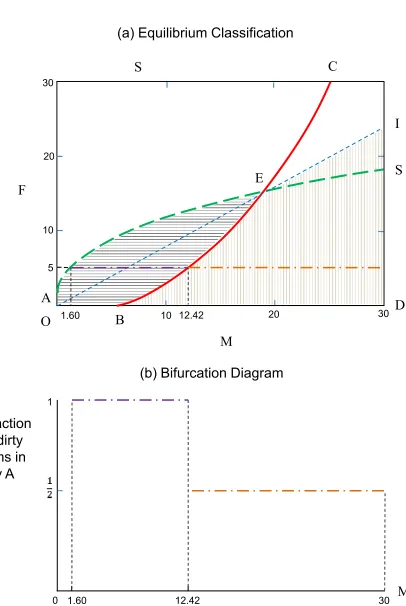
Remark 6: (Equilibrium Classi…cation and Bifurcation Diagram) It is possible to delineate
nu-merically a diagram in (M; F), namely the exogenous measure of dirty …rms and the exogenous
…xed cost tax revenue, that shows how changes in the values of (M; F) result in di¤erent types
1 0If there is no tax and both industries have (di¤erent) CRS production functions (with no Romer externality) but
of equilibria, i.e. integrated versus strati…ed. Speci…cally, we set = = = 0:5, = = 1,
= 0:1 and = 0:02. We can then vary the values of each of M and F from 0 to 30. As shown
in Figure 5(a), strati…cation is more pro…table than integration for lower values of M and higher
values ofF: the indi¤erence boundary between the two con…gurations is given by^BEC. Of course, a con…guration can be supported only under positive pro…t, which is met for the area underAES] in the case of strati…cation and for the area underOEI] in the case of integration. Thus, a strati…ed equilibrium arises in the area of OAEB (shaded with horizontal lines) whereas an integrated
equi-librium emerges in the area ofBEID (shaded with vertical lines). We now set F = 5 and vary the
measure of dirty …rms, M. As long as M > 1:60, a nondegenerate equilibrium exists where …rms
earn su¢cient pro…ts to pay for the pollution tax. Over the rangeM 2(1:60;12:42), the equilibrium
con…guration is strati…ed and the fraction of dirty …rms in cityAis one. As …rms continue to enter,
the equilibrium con…guration becomes integrated and the fraction of dirty …rms in city Adrops to
1
2. This is depicted in the bifurcation diagram, Figure 5(b).11
[Insert Figures 5(a,b) here]
The intuition behind the equilibrium con…guration of …rms under various parameter values is as
follows. At moderate levels of …xed tax cost F, if there are few dirty …rms M, they must cluster
together to be able to pay the tax. However, as the number of dirty …rms increases, enough pro…t is
generated to allow them to separate into halves and a¤ord to pay the tax out of pro…ts. Although
they could conceivably generate even more pro…t if they strati…ed, the missing items are the level
of pollution and the wage. With many dirty …rms, the level of pollution in a strati…ed con…guration
is high, so the wage rate must also be high to attract workers, and this makes such a con…guration
impossible. For other parameter values that we have not discussed, for example if the number of
dirty …rms is low but the …xed tax cost is moderate or high, the dirty …rms will all shut down even
with the Inada condition on utility. If they all produce just a little, pro…ts are insu¢cient to pay
the tax.
Remark 7: (Reexamining the Role of Agglomerative Externalities) In our benchmark setup, by
incorporating a regional-speci…c agglomeration externality following the Romer (1986) convention,
dirty goods production exhibits private decreasing-returns-to-scale and social
constant-returns-to-scale. Social constant returns simplify the analysis greatly, enabling a clean analysis of the
equi-librium con…guration, namely integration versus strati…cation. Nonetheless, the parameter on
the one hand captures the degree of externality and on the other hand measures the magnitude of
producer rent. Let us examine how the magnitude of would a¤ect the result by looking at the
two inequalities in Condition S-10
separately:
1 + F
(1 ) M1 < M
1 1
F
1
M1 1
F
1
< 2
2
It is clear that higher (lower producer rent and lower magnitude of externality) implies that the
…rst inequality of the strati…cation condition is less likely to hold. Both the left hand side and the
right hand side of the second inequality are, however, lower and the net e¤ect on the likelihood
of strati…cation is thus ambiguous. For su¢ciently high (for example, taking the extreme case
as ! 1), the …rst inequality always fails to hold while the second always holds. Intuitively,
as the region-speci…c agglomeration externality diminishes, dirty …rms will have less incentive to
cluster. However, when becomes too high, dirty …rms can never generate enough rent to cover
…xed costs regardless of the underlying con…guration (integration versus strati…cation). This is
because we cannot separate the role of the agglomerative externality from producer rent.12 We can
further resort to our numerical example, presented in Remark 6 above, to discuss how equilibrium
classi…cation changes in response to .
[Insert Figure 6(a,b) here]
From Figure 6(a), we can see that, under the benchmark parametrization, when < 0:6273 and
F takes intermediate values falling between the long dashed curve and the solid curve, a strati…ed
con…guration arises in equilibrium; when is higher than the critical value andF takes low values
falling below both the the solid curve and the dashed curve, an integrated con…guration emerges.
As increases, the range of F that can support a nondegenerate competitive spatial equilibrium
(namely one with positive dirty good production and …nite relative prices) narrows. We can also
reproduce the bifurcation diagram 5(b) in Figure 6(b): it indicates that, given the benchmark values
F = 5 and M = 12:571, the equilibrium con…guration is strati…ed over the range 2(0;0:5000);
the equilibrium con…guration turns integrated when 2 (0:5000;0:7220), and only a degenerate
competitive spatial equilibrium (with no dirty good production and in…nite relative price) exists
when continues to rise, exceeding 0:7220.
1 2In order to separate these two channels (producer rent and magnitude of externality), one must give up social
constant returns, assuming instead social decreasing returns: f ne i
y(j); Nyi = [niy(j)] 1[Nyi] 2; >0, 1; 22(0;1)
Remark 8: (On Endogenous Choice of Production Technologies) In the benchmark economy, we
have followed an Arrow-Debreu convention by assuming that producers are endowed with speci…c
technologies for producing particular goods. One may inquire what happens if producers are allowed
to make an endogenous choice of production technologies (clean versus dirty). Consider the model
modi…ed so that a potential producer can choose between clean and dirty good production, followed
by location choice and then production. Then the value of being a clean good producer (zero pro…t)
must be equal to the value of being a dirty good producer, implying: maxf (I); (S)g= 0, where
(I) = M
2 (1 )f0(2=M) (2=M(I))ny(I) (2=M(I))
i
(S) = M u0
f(1=M)M2ny(S) (1=M(S))ny(S) (1=M(S)) i
Let the equilibrium mass of dirty …rms as a result of free entry be denoted asM (I) and M (S),
respectively, for the cases of integration and strati…cation. Thus,
(2=M (I))
2=M (I) =
i
ny(I)
(1=M (S))
1=M (S) =
i
ny(S)
Recall from our discussion of the bifurcation diagram that asM rises, (ee) would increase ineand hence (22=M=M)) would become more likely to dominate (11=M=M). Using this property and manipulating (see the Appendix), we arrive at:
M (I) = 2
"
2F
1
1 #11
M (S) = [ (1 ) + F]
(1 )2 F
1 1 1
This is familiar from the monopolistic competition literature with endogenous entry of …rms, as
in the work by Melitz (2003). While one may impose constraints in various ways to determine
the equilibrium outcome, a land requirement is natural in our economy (as proposed by Helpman,
1998). Suppose there is a …xed land requirement for all households and …rms, each at an inelastic
unit normalized to one (which can be justi…ed as an equilibrium outcome as in Berliant, Peng and
Wang, 2002). Consider the public land ownership structure delineated in Fujita (1989, pp. 60-61)13
with a total supply of L > 2 in the entire local economy. Then the total land demand is: 2 +M
(clean …rms of mass one + dirty …rms of massM + households of mass one). It is straightforward
1 3The public land ownership model features land rent collections that are refunded equally to all inhabitants of a
to see that the necessary and su¢cient condition for the strati…ed con…guration to arise as the only
equilibrium outcome is:
2 +M (S) L <2 +M (I)
The above inequalities can be manipulated to yield (see the Appendix):
1 + F
(1 )
(1 )1 (L 2)1
F1 <
22
(36)
which can hold true only if
1 + F
(1 ) <
22
(37)
The latter inequality is satis…ed when is su¢ciently small (i.e., with a su¢ciently strong spillover
externality). Given Condition (37), then Condition (36) ensures that the equilibrium is strati…ed.
This condition requires that (i) the …xed payment F is not too large (otherwise, too many …rms
must cluster, implying that land demand exceeds land supply) and (ii) land supply is not too large
(otherwise, even an integrated equilibrium can be supported). Notice that neither the …rms’ nor
the households’ optimization problems change with the introduction of the land market. This is
because, for producers, the same amount of land rent is added and subtracted from pro…ts, whereas
for consumers the same amount of land rent is added to both sides of the budget. In short, adding
endogenous technology choice by allowing potential producers choose between clean and dirty good
production would not alter our main …ndings once we introduce a simple land market under public
ownership with an appropriate land supply satisfying Condition (36).
6.2 Linear Pollution Tax Regime
We turn next to examining the case of a linear pollution tax. Consider,
Condition S-20
: (Strati…ed Equilibrium)
(1 t) + M L
(1 ) <
M (1 t)2 (1
L )
1 <21
We now have:
Proposition 3: (Strati…ed Equilibrium under Linear Pollution Tax) Consider a local economy in
which pollution production is not too severe and pollution disutility is not too high, in other words
is su¢ciently small, and Condition R-2 is met. Then, under a linear pollution tax regime with
Condition S-20
7
Can Pareto Optimum Be Price Supported?
Since individuals are ex ante identical, we restrict our attention to within-region-equal-treatment
Pareto optimum in the sense that all households within a given region reach an identical indirect
utility level and consume the same bundle. Such a Pareto optimum must satisfy the following
constraints:
xi(j) = nix(j); i=A; B; j2[0; ki]
yi(j) = Nyif n
i y(j)
Ni y
!
; i2A; B; j2[0; mi]
Nxi =
Z ki
0
nix(j)dj, Nyi =
Z mi
0
niy(j)dj, NxA+NxB+NyA+NyB= 1
X
i=A;B
Nicix = X
i=A;B Z ki
0
xi(j)dj, X i=A;B
Niciy = X
i=A;B Z mi
0
yi(j)dj
where the …rst two equations specify production technologies, the third gives labor material balance
and the population identity, and the last represents commodity material balance. Such Pareto
optima are found by solving the following optimization problem:
maxUA = cAx
Z mA
0
yA(j)dj+u(cAy)
s.t. UB = cBx
Z mB
0
yB(j)dj+u(cBy) =U
and the above technology and material balance constraints.
We consider equilibria with linear taxes in the next two subsections.
Remark 9: (Pareto Optimal Con…guration) It is natural to inquire at this point whether, for
given parameters, the Pareto optimum features an integrated or strati…ed con…guration. Indeed,
although it is not central to our analysis, in general it depends on the comparison of utility from
dirty good production and pollution damage in a region with half or all of the dirty …rms. In our
quasi-linear setting, it amounts tou(2f(2=M)) f(2=M)for an integrated con…guration compared
withu(f(1=M)) f(1=M) for a strati…ed con…guration.
7.1 Case I: Integrated Optimum
At an integrated optimum, we have all interior allocations. We can establish:
Theorem 3: (Equilibrium Support of Integrated Con…guration) Consider a local economy in
is su¢ciently small, and Condition R-2 is met. Then, the Pareto optimum with an integrated
con…guration can be supported by a competitive spatial equilibrium under the following marginal tax
rate: =f1 + 2 =[ f0
(2=M)]g 1.
Intuitively, the higher the pollution damage (captured by larger ) is, the greater the marginal
pollution tax will be.
7.2 Case II: Strati…ed Optimum
At a strati…ed optimum, we have: kA=mB= 0. We can establish:
Theorem 4: (Suboptimality of Strati…ed Equilibrium) Consider a local economy in which pollution
production is not too severe and pollution disutility is not too high, in other words is su¢ciently
small, and Condition R-2 is met. Then, a strati…ed competitive spatial equilibrium is suboptimal
with over-employment and over-production in the dirty goods sector relative to the strati…ed Pareto
optimum.
Thus, a strati…ed equilibrium can never reach Pareto optimality by means of a linear pollution tax
(which encompasses Pigouvian taxation). In fact, the equilibrium employment in the dirty sector
under the strati…ed con…guration is always too large, implying that dirty goods and pollution are
both over-produced. Such an over-polluting equilibrium outcome can never be corrected by a linear
pollution tax.
To understand the result, it is best to refer to Figure 7, where we plot the downward-sloping
after-tax MPL locus in the top panel and repeat the locational equilibrium diagram (the top panel
of Figure 3) in the bottom panel of Figure 7. A high marginal tax will shift down the after-tax
MPL locus without altering any other curves. Thus, the only change is the corresponding reduction
in the dirty industry wage, wA. As long as wA > still holds after the tax increase, the lower
wage will be fully o¤set by the tax and pro…t redistribution, keeping consumers in region Aas well
o¤ as before the tax increase. This is equivalent to saying that although dirty good demand is
elastic, dirty good supply is perfectly inelastic. As a result, dirty good employment and production
in strati…ed equilibrium remain at levels higher than the respective optimum quantities, regardless
of the linear pollution tax levied.
[Insert Figure 7 here]
Another way of interpreting our welfare results is as follows. The same number of distortions
and tax instruments are available no matter the equilibrium con…guration of …rms, so that one
taxes independent of the equilibrium con…guration. However, the integrated Pareto optimal
con-…guration has the unique feature that it is symmetric across locations, so the distortion associated
with migration is not present. Thus, one fewer instrument is needed to support the integrated
con…guration, in contrast with the strati…ed con…guration.
In the conventional literature, Pigouvian taxes (a special form of a linear tax without the
lump-sum component) need not work in practice due to the di¢culty of computing marginal damages
at the optimum (Baumol 1972), or when …rms have monopoly power so that they can transfer
the tax burden (Buchanan and Tullock, 1975), or when oligopolistic …rms have dynamic strategic
interactions (Benchekroun and Van Long 1998), or when lobbying groups care about the distribution
of income in political games (Aidt 1998)). In our paper, assuming away all of these issues, we show
that even a generalized Pigouvian tax as proposed by Carlton and Loury (1980) cannot restore …rst
best under a static, competitive environment, when we allow locational choice with endogenous
clustering.
Whereas the linear pollution tax cannot correct equilibrium ine¢ciency, it should be noted
that an appropriate redistribution scheme may do the job. In particular, consider a lump-sum
redistribution from polluted regionA to clean regionB. This induces U to shift down and hence
equilibrium employment in the dirty industry to fall. Thus, as long as is not too large, there
exists an appropriate level of such a redistribution to support the Pareto optimal level of dirty
industry employment as an equilibrium.
8
Concluding Remarks
In this work, we have shown how a …xed charge component of a tax system can cause agglomeration
of polluting …rms as an equilibrium phenomenon. We have also established that whereas an
integrated Pareto optimum can be supported by a competitive spatial equilibrium with a linear
pollution tax, a strati…ed Pareto optimum cannot. Regardless of the linear pollution tax schedule,
a strati…ed equilibrium is always over-polluted compared to the optimum. To support the strati…ed
Pareto optimum, however, an e¤ective (but practically not implementable) policy prescription is
to redistribute the pollution tax revenue from the dirty to the clean city residents. Such a policy
will induce migration to the clean city, thereby reducing production of the dirty good and thus of
pollution.
In this paper, we have considered only equilibrium con…gurations that are completely strati…ed
locations. One may inquire whether other con…gurations may emerge in equilibrium. The answer is
positive: it is possible that one city is mixed with both clean and dirty industries present, whereas
another has only the clean industry. In this con…guration, clean industry workers must have equal
utility across locations and all workers must have the same wage in the city with mixed industries.
Under the Ricardian technology where clean workers are paid an exogenously …xed wage, the two
equalization conditions can be met only in knife-edge cases. It is therefore innocuous to ignore this
partially integrated con…guration.
Many extensions of the model are possible. For example, global or interregional pollution could
be present in addition to the local pollution we have considered. Naturally, agglomeration is a
product of local pollution, as global pollution a¤ects everyone in the same way. Aside from the
extension to endogenous technology choice delineated in Remark 8, we have refrained from adding
land to the model for tractability reasons. Future work should proceed in this direction.
Capital-ization of pollution damages and lump-sum transfers to localities could change the results. It would
References
[1] Aidt, T.S., 1998. Political internalization of economic externalities and environmental policy.
Journal of Public Economics 69, 1-16.
[2] Baumol, W. J., 1972. On taxation and the control of externalities.American Economic Review
62, 307-322.
[3] Benabou, R., 1996a. Heterogeneity, strati…cation and growth.American Economic Review 86, 584-609.
[4] Benabou, R., 1996b. Equity and e¢ciency in human capital investment: The local connection.
Review of Economic Studies 63, 237-264.
[5] Benchekroun, H. and N. Van Long, 1998. E¢ciency inducing taxation for polluting oligopolists.
Journal of Public Economics 70, 325-342.
[6] Bergstrom, T. and R. Cornes, 1983. Independence of allocative e¢ciency from distribution in
the theory of public goods. Econometrica 51, 1753-1765.
[7] Berliant, M., S. Peng and P. Wang, 2002. Production externalities and urban con…guration.
Journal of Economic Theory 104, 275-303.
[8] Buchanan, J. M. and G. Tullock, 1975. Polluter’s pro…ts and political response: Direct control
versus taxes. American Economic Review 65, 139-147.
[9] Carlton, D.W. and G.C. Loury, 1980. The limitation of Pigouvian taxes as a long-run remedy
for externalities.Quarterly Journal of Economics 95, 559-567.
[10] Chen, B., S. Peng and P. Wang, 2009. Intergenerational human capital evolution, local public
good preferences, and strati…cation. Journal of Economic Dynamics and Control 33, 745-757.
[11] Chen, B., C. Huang and P. Wang, 2012. Strati…cation by environment. Journal of Public
Economic Theory 14, 711-735.
[12] Chipman, J.S. and G. Tian, 2012. Detrimental externalities, pollution rights, and the ‘Coase
theorem’. Economic Theory 49, 309-327.
[13] Fujita, M., 1989. Urban Economic Theory: Land Use and City Size. New York, Cambridge
University Press.
[14] Hartwick, J., U. Schweizer and P. Varaiya, 1976. Comparative statics of a residential economy
[15] Helpman, E., 1998. The size of regions, in D. Pines, E. Sadka and Y. Zilcha (eds.), Topics in
Public Economics. New York, Cambridge University Press, pp. 33-54.
[16] Karp, L., 2005. Nonpoint source pollution taxes and excessive tax burden.Environmental &
Resource Economics 31, 229-251.
[17] Markusen, J.R., E.R. Morey and N. Oleviler, 1995. Competition in regional environmental
policies when plant locations are endogenous. Journal of Public Economics 56, 55-77.
[18] Melitz, M.J., 2003. The impact of trade on intra-industry reallocations and aggregate industry
productivity. Econometrica 71, 1695-1725.
[19] Nechyba, T., 1997. Existence of equilibrium and strati…cation in local and hierarchical Tiebout
economies with property taxes and voting. Economic Theory 10, 277-304.
[20] OECD, 1994.Managing the Environment: The Role of Economic Instruments. Paris, OECD.
[21] Peng, S. and P. Wang, 2005. Sorting by foot: ‘travel-for’ local public goods and equilibrium strati…cation.Canadian Journal of Economics 38, 1224-1252.
[22] Picard, P.M. and T. Tabuchi, 2010. Self-organized agglomerations and transport costs.
Eco-nomic Theory 42, 565-589.
[23] Pigou, A. C., 1920.The Economics of Welfare. London, Macmillan.
Appendix
Proof of Theorem 1: A condition su¢cient to show that the strati…ed con…guration is an
equilibrium but the integrated con…guration is not is:
(I)<0< (S)
That is, the dirty …rms only operate under strati…cation. From (29) and (32), in turn, we need the
following inequality condition:
1
4e(2=M)ny(I)<
F
M2 <e(1=M)ny(S)
Whenny(I)< ny(S), the above inequality holds under Condition S-1, which can be met only under
Condition R-1. Sinceny(I)andny(S)are endogenous, we must further investigate their magnitudes
[image:32.612.178.457.478.533.2]in order to establish precise su¢cient conditions on primitives. This can be accomplished utilizing
Figure 4, by comparing the positions of pointEI and point ES. We can see from the top panel of Figure 4 that, as long as is not too large, we can have ny(I) < ny(S) (as shown in the bottom
panel of Figure 4). Given this and Condition R-1, we can always choose F to satisfy Condition
S-1, which subsequently ensures the existence of a strati…ed con…guration but not the integrated
con…guration as an equilibrium outcome, as illustrated diagrammatically where ny(S) is pinned
down by Figure 4 with Conditions R-1 and S-1 met as in Figure 7(a).
Proof of Theorem 2: In this case, the pro…ts generated by each dirty …rm under integrated and
strati…ed con…gurations become:
(I) = M
2 (1 t)f0( 2
M)
[(1 t)e( 2
M)ny(I)
2
ML]
(S) = M u0
[f( 1
M)M
2n
y(S)][(1 t)e( 1
M)ny(S)
1
ML]
Similar to the …xed tax case, here is a su¢cient condition to ensure that the strati…ed con…guration
is an equilibrium but the integrated con…guration is not:
(I)<0< (S)
which can be rewritten as the following inequalities:
1
2e(2=M)ny(I)<
L
(1 t)M <e(1=M)ny(S)
Under Condition R-2, as shown in Figure 7(b) and the circumstances delineated by Figure 4,