A factor augemented model of markup on mortgage loans in Poland

Munich Personal RePEc Archive

A factor-augemented model of markup

on mortgage loans in Poland

Bystrov, Victor

University of Lodz

9 September 2013

Online at

https://mpra.ub.uni-muenchen.de/49683/

A Factor-Augmented Model of Markup

on Mortgage Loans in Poland

Abstract

The paper describes the results of estimation of a factor-augmented vec-tor auvec-toregressive model that relates the markup on mortgage loans in na-tional currency, granted to households by monetary financial institutions, and 1-month inter-bank rate that represents the cost of funds for financial institutions. The factors by which the model is augmented, summarize in-formation that can be used by banks to forecast interest rates and evaluate macroeconomic risks. The estimation results indicate that there is a sig-nificant relation between the markup and the changes in 1-month WIBOR. This relation can be interpreted as evidence of incomplete transmission of the monetary policy shocks to mortgage rates set by monetary financial institutions. The policy shocks are partially absorbed by changes in the markup.

JEL: C32, C53, E43, E44

Keywords: factor models, interest rates, pass-through, markup

1

Introduction

An interest rate pass-through model represents a relation between retail rates set

by monetary financial institutions for households and firms and a policy rate or a

wholesale market rate representing cost of funds for financial institutions. Before

the emergence of the financial crisis, the empirical literature on the interest rate

pass-through focused on the estimation of bivariate models relating a retail rate

speed of the pass-through were considered as indicators of the effectiveness of

monetary policy.

Under conditions of financial turmoil, the effect of policy rates and short-term

market rates on retail rates has become weaker, and the conventional models of the

pass-through have become poor representations of the monetary policy

transmis-sion. An augmentation of the conventional models is needed in order to account for

additional information that monetary financial institutions consider when settting

retail rates for households and firms.

In this paper we consider a factor-augmented vector autoregressive (FAVAR)

model that explains deviations from the long-run equilibrium defined by a

con-ventional model of the pass-through for mortgage rates in Poland. A concon-ventional

model is based on the assumption of a constant markup of a retail rate over a

wholesale rate. Persistence changes in the markup imply deviations from the

equilibrium. The FAVAR estimated in this paper, measures relations between the

markup, changes in a wholesale rate, and a few common factors that are estimated

using a large panel of macroeconomic and financial indicators.

The empirical model is motivated by a theoretical forward-looking model which

describes a relation between the markup and the expectations formed by monetary

financial institutions. The common factors summarize information that can be

used by monetary financial institutions in the evaluation of macroeconomic risks

and the forecasting of future interest rates.

The paper is organized as follows. In the next section we describe a simple

theoretical model of the pass-through. Section 3 includes a description of the

econometric model. Data description is given in Section 4. The estimation results

2

Aggregation, expectations and the pass-through

Monetary Financial Institutions (MFI) Interest Rates (MIR) statistics adopted in

the EU countries, including Poland, provides synthetic retail bank rates that are

aggregated into a few broad categories defined by the type of a product and its

maturity (e.g., loans for house purchases over 1 year and up to 5 years maturity).

The aggregation is performed by reporting agents (monetary financial institutions).

Therefore, no systematic statistical data are available for individual products of

exact maturity.

The economic literature on the interest rate pass-through uses these retail rates

to match them with money market rates or government bond yields (wholesale

rates) defined for specific maturities (see, e.g., de Bondt 2005). As there is no exact

matching of maturities between retail rates and wholesale rates, two approaches

are commonly used: either a retail rate is matched to a short-term money market

rate approximating a policy rate (like 1 or 3-month EURIBOR), or an appropriate

wholesale rate is chosen on the basis of correlation analysis among those rates

which are closest to a given retail rate in maturity. A notable exception is the

study by Sorensen and Werner (2006) who construct synthetic wholesale rates.

The first approach ignores the maturity transformation and is only valid if there

is a stable relation between short-term money market rates and long-term bond

yields. The second approach uses an ad hoc method which may match different

wholesale rates over different sub-samples of data.

A MIR rate is a synthetic rate representing a weighted average of retail rates

rt = τ

∑

τ=τ

ωτrt(τ),

where rt(τ) is a retail rate of maturity τ (here, maturity means period of interest

rate fixation), τ is the minimal maturity and τ is the maximal maturity of retail

rates which are included in the synthetic rate rt, ωτ is the weight of a rate of

maturity τ. The weights ωτ, τ =τ , τ + 1, ...τ, are not systematically reported by

MFIs.

If monetary financial institutions were matching maturities of retail and

whole-sale rates, then the baseline pass-through equation would have the form,

rt=ν+β τ

∑

τ=τ

ωτmt(τ), (1)

where mt(τ) is a wholesale rate on a debt obligation of maturity τ, β is the

pass-through coefficient, andνis the bank mark-up. The parametersνandβare said to

be determined by the demand elasticity and the market structure (de Bondt 2005).

If β < 1, then the through is said to be incomplete. The incomplete

pass-through is explained by microeconomic factors such as low market competitiveness

and credit rationing (see, inter alia, Winker 1999; Kot 2003; Chmielewski 2004;

Gambacorta 2006; Sorensen and Werner 2006). However, in this paper we consider

a macroeconomic model of the incomplete pass-through.

If MFIs do not match maturities, but rely on the short-term financing, then

they have to forecast a short-term wholesale rate and determine a risk premium

in order to set a retail rate. Let us consider a modification of the linearized

expectations model proposed by Shiller (1979), which relates a wholesale rate

mt(τ) =φt(τ) +

1−γ 1−γτ

τ−1 ∑

h=0

γhEtmt+h(1), (2)

whereφt(τ) is a time-varying risk premium,γ is a discount factor, and Etmt+h(1)

is the expectation of the one-period rate.

Substituting (2) in (1), we obtain

rt=ν+β τ

∑

τ=τ

ωτ

[

φt(τ) +

1−γ 1−γτ

τ−1 ∑

h=0

γhEtmt+h(1)

]

.

After rearrangement, using ∆(h)_m

t+h(1) =mt+h(1)−mt(1):

rt=

[

ν+β

τ

∑

τ=τ

ωτφt(τ)

]

+βmt(1) +β

[_∑τ

τ=τ

ωτ

1−γ 1−γτ

τ−1 ∑

h=1

γhEt∆(h)mt+h(1)

]

.

The equation can be rewritten as

rt=µt+βmt(1) + τ−1 ∑

h=1

δhEt∆(h)mt+h(1),

where

µt=

[

ν+β

τ

∑

τ=τ

ωτφt(τ)

]

, and δh =

    

β∑τ_τ=τωτ₁1₋−_γγτγ

h_{, h≤τ −1}

β∑τ_τ=h+1ωτ₁1₋−_γγτγ

h_{, h≥τ}

.

The synthetic retail rate rt can be expressed as a function of a spot short-term

rate and expected changes in the short term rate up to the maximal maturity of

retail products included in the synthetic rate rt. The residual variability of the

retail rate can be explained by the fluctuations in the risk premium.

In the Polish market of mortgage loans, the predominant pricing mechanism

WIBOR (Warsaw Inter-Bank Offered Rate) plus a markup. Such pricing

mech-anism implies that the long-term value of the pass-through coefficient β should

be equal to one. The markup, defined as a difference between the retail rate on

mortgage loans and a 1-period WIBOR, is given by

zt=rt−mt(1) =µt+ τ−1 ∑

h=1

δhEt∆(h)mt+h(1),

where τ is the maximal period of interest rate fixation.

In this model, persistent changes in the markup zt are caused by changes in

the evaluation of risk and revisions of forecasts by monetary financial institutions.

The persistent changes in the markup mean ineffectiveness of the monetary policy

based on the regulation of interest rates, as monetary financial institutions do not

fully transmit changes in wholesale (market) rates to retail rates, but partially

absorb those changes through changes in the markup.

3

Econometric Model

In this paper a dynamic factor model is employed to summarize information that

can be used by MFIs in making projections of future interest rates and evaluation

of risk. In a similar study, Banerjee, Bystrov and Mizen (2013) estimated a

pass-through model where recursive forecasts of a market rate were included into a

dynamic regression. The forecasts were based on a factor model of the yield curve.

Though the study confirmed the importance of forecasts in the retail rate setting,

the forecasts were based on the information contained in the yield curve only and

the risk premium was assumed to be constant. The performance of the model

financial variables that might be useful in the forecasting of market rates and the

evaluation of risk.

We model expectations of MFIs as based on a dynamic factor model which

represents an extensive set of macroeconomic and financial variables by a few

common factors:

Xt= ΛtFt+et,

where Xt is (N ×1) vector of observed stationary macroeconomic and financial

indicators, Ft is (R ×1) vector of unobserved common factors (R << N), Λt is

(N×R) matrix of loadings, and et is (N ×1) vector of idiosyncratic components.

A factor forecast can be constructed as a direct projection on the estimated

common factors, their lags and lags of the forecast variable:

∆(h) b

mt+h|t(1) =a

(h)

t + K

∑

k=0

b(_kth)′Fb_t(₋t)_k+

L

∑

l=0

c(_lth)∆mt−l(1), h= 1,2, ..., τ −1,

where ∆(h)_mb

t+h|t(1) is a forecast of h-period change in a one-period market rate

conditional on the information available at time t.

MFIs can use a variety of macroeconomic and financial indicators to forecast

future interest rates. The information contained in these indicators can be

parsi-moniously summarized by few common factors, and the factor forecasts can serve

an approximation of the expectations formed by MFIs. However, the

informa-tion, summarized by the common factors, may also be used in the evaluation of

macroeconomic risks and the determination of the risk premium (µt).

Therefore, the inclusion of factor forecasts in a pass-through model, while

can be time-varying and dependent on the macroeconomic indicators which are

included in the factor model. In this paper, a dynamic model of the pass-through

is augmented by the estimated common factors, assuming that the information,

which is summarized by these factors, may determine both expectations and the

risk premium.

A bivariate vector autoregression, including a measure of markup, zt, and a

change in a market rate, ∆mt(1), is augmented by a few factorsFbtextracted from

a large number of macroeconomic and financial indicators:

  Fb

(T)

t

∆mt(1)

zt

 =



 αΦ((LL))′ _a(0_{L) b(}0_L)

β(L)′ _{c(L) d(L)}

 

  Fb

(T)

t−1

∆mt−1(1)

zt−1  +

  εη1tt

ε2t

 ,

whereFbt(T) is (R×1) vector of estimated common factors; Φ(L) is (R×R) matrix

lag polynomial;α(L) andβ(L) are (R×1) vector polynomials;a(L),b(L),c(L), and

d(L) are scalar polynomials. The common factorsFtare assumed to be exogenous

with respect to markup zt and differenced market rate ∆mt(1). Therefore, zero

restrictions are imposed on the lags of zt and ∆mt(1) in the equations for the

common factors.

The common factors are estimated using the principal components

estima-tor. Bai and Ng (2006) provide central limit theorems and confidence intervals

for inference in factor-augmented regressions. We implement Bai and Ng (2006)

methodology: parameters of the factor-augmented regressions are estimated

us-ing the least squares estimator and heteroscedasticity-consistent standard errors

are computed to account for consequences of including generated regressors in the

4

Data Description

The FAVAR model is estimated using monthly data from January 2004 to

De-cember 2012. The markup is computed as a difference between the average rate

on outstanding amounts on mortgage loans granted in national currency and the

monthly average of 1-month WIBOR. It is a synthetic measure of markup that

can only be interpreted as an approximation of the actual markup set by MFIs.

The mortgage rate is extracted from the Monetary and Financial Statistics of the

National Bank of Poland. Figure 1 shows the time series plot of two series (with

means subtracted).

The dynamic factor model is estimated using monthly data from January 2001

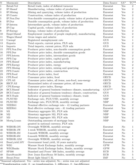
to December 2012. The data include 49 time series covering industrial production,

prices, exchange rates, interest rates, monetary aggregates, stock exchange indices

and leading business indicators (see Table 1 in the Appendix). The series were

extracted from a databases of a few institutions: the National Bank of Poland

(NBP), the Central Statistical Office of Poland (GUS), the Warsaw Stock Exchange

(GPW), Eurostat, the European Central Bank (ECB), the OECD, and the IMF.

The composition of the data panel is aimed to provide a balanced representation

of all sectors of the Polish economy.

Prior to estimation of the factor model, the data were processed using Stock

and Watson (1999) methodology. First, all series that were modelled as generated

by integrated processes, were transformed to stationary series, using differences

or log-differences. Second, all non-financial time series were seasonally adjusted

using Census X12-ARIMA procedure. Third, outliers exceeding the interquartile

sub-sequently substituted by estimates obtained using the expectation-maximization

(EM) algorithm. Fourth, all series were standardized to have zero mean and unit

variance.

5

Estimation Results

The common factors were estimated using the principal component estimator.

First, the estimation was performed a panel of series including no missing values.

Second, missing values were interpolated using the EM algorithm and the factors

were estimated using the whole panel.

Initially, ten common factors were estimated. Of those, six factors were selected

using a threshold of at least 5 percent of the total variance explained by each

se-lected factor (for an application of such criterion, see Forni and Reichlin 1998).

The final FAVAR obtained in the model selection process, included only four

fac-tors. These four factors explain 50 percent of the total variance in 49 time series.

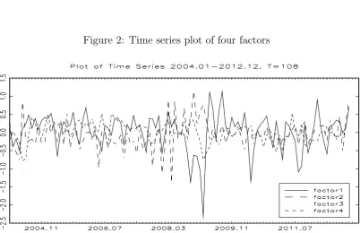
The time series plot of these factors is shown in Figure 2 and the loadings of these

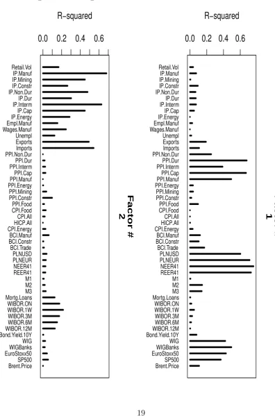
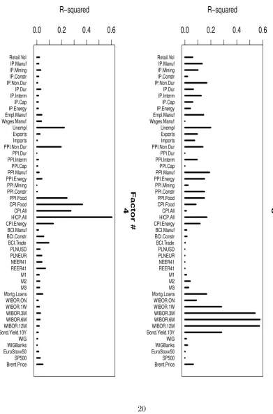
factors onto individual time series are presented in Figures 3-4. The first factor

loads on nominal indicators: producer price inflation, returns on exchange rates

and stock indices. The second factor loads on indicators of industrial production

and foreign trade. The third factor is correlated with interest rates and the fourth

factor has the highest correlation with indicators of consumer price inflation.

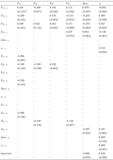
The selection of the FAVAR model was carried out using System SER

(Se-quential Elimination of Regressors) procedure based on the Bayesian Information

Criterion (Br¨uggemann and L¨utkepohl 2001). The initial model included six

fac-tors and six lags of facfac-tors, the markup and the difference of 1-month WIBOR.

Table 2).

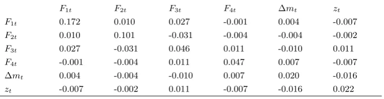
The eigenvalues of the companion matrix of the estimated FAVAR and the

covariance matrix of disturbances are reported in Table 3. All eigenvalues of the

companion matrix are less than one in modulus, which means that the estimated

FAVAR is stable (there are no unit or explosive roots).

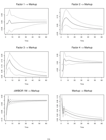
The orthogonalized impulse responses of the differenced 1-month WIBOR and

the mortgage markup are presented in Figures 5 and 6. The figures show the 95

percent joint bootstrap confidence bands obtained using the neighbouring paths

method proposed by Staszewska (2007) (see also Staszewska-Bystrova 2011). The

joint band contains the entire response function constructed for a given response

horizon with probability 0.95.

The assumed ordering of variables in the FAVAR means that common factors

can have an immediate effect onto the 1-month WIBOR and the markup. However,

the 1-month WIBOR and the markup have no immediate effect on the common

factors. This is consistent with the interpretation of the common factors as

ex-ogenous latent variables that describe a state of the economy. The ordering of the

variables also implies that the 1-month WIBOR may have an immediate impact

onto the markup, but not vice versa.

Figure 5 shows the orthogonalized impulse responses of the markup, zt, to

shocks in the common factorsF1t,F2t,F3t, andF4t, and in the differenced 1-month

WIBOR, ∆mt(1). Each shock is equal to one standard deviation of residuals in

the estimated equation for a corresponding variable. An impulse to the differenced

1-month WIBOR, ∆mt(1), implies a significant negative shock to the markup, zt,

which slowly converges to the previous level afterwards. It means that if the level

decreases temporarily: a part of the increase in the WIBOR is not transferred to

an increase in mortgage rates - it is absorbed by a decrease in the markup.

There are significant impulse responses of the markup to factors 2, 3, and

4, which are correlated with the growth rates of industrial production, changes in

interest rates, and consumer price inflation correspondingly. The direction of these

effects should be interpreted with a precaution though, as factors are identified

up to a linear transformation, and additional restrictions have to be imposed to

admit a structural interpretation of these impulse responses. However, it can

be concluded that one has to control for other macroeconomic indicators when

measuring the response of the markup to a short-term market rate.

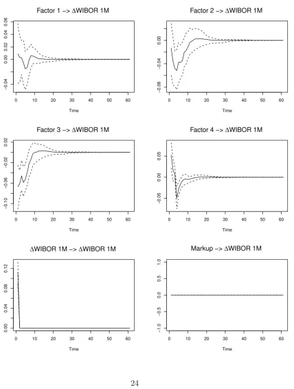
The orthogonal impulse responses of the 1-month WIBOR are shown in Figure

6. There are significant responses of the differenced 1-month WIBOR to shocks

in factors correlated with growth rates of industrial production, changes in other

interest rates, and consumer price inflation. These factors summarize information

of potential use in the forecasting of 1-month WIBOR and the determination of

the markup which is set on mortgage loans by MFIs. There is no feedback from

the markup to 1-month WIBOR, as lags of the markup are excluded from the

equation for the differenced WIBOR by the model selection procedure, and the

markup is assumed to have no instantaneous effect on the WIBOR.

In order to investigate the parameter stability of the estimated FAVAR model,

we implement the Andrews (1993) and the Andrews-Ploberger (1994) tests, which

are based on the supremum Wald statistic and the average exponential Wald

statis-tic respectively. It was demonstrated in several studies (see Stock and Watson

1998; Hansen 2000; Cogley and Sargent 2005) that these tests have the highest

dy-namic regressions.

Following Stock and Watson (1996), we implement a heteroscedasticity-robust

version of these tests and compute bootstrapped critical values to account for a

small sample size. The Andrews the Andrews-Ploberger tests are not based on

the assumption of a specific date of structural change, but evaluate stability of

the parameters over a window of observations. We selected a symmetric window,

trimming 25 percent of the observations at the beginning and at the end of the

estimation sample. As a result, the stability of parameters was tested over the

period from May 2006 to September 2010. A choice of a larger window would lead

to computational instability of the least square estimator.

Table 4 reports computed test statistics together with bootstrapped and

asymp-totic critical values for the 5 percent level of significance. The results are provided

for each equation of the FAVAR model and for the model as a whole. The test

statistics of both tests are smaller than bootstrapped and asymptotic critical

val-ues for all equations of the model. Therefore, the null hypothesis of parameter

stability cannot be rejected given the significance level of 5 percent. No evidence

of parameter instability in the FAVAR model is found.

6

Conclusions

In this paper, a factor-augmented VAR model is used to explain the relation

be-tween changes in 1-month WIBOR and the markup on mortgage loans in national

currency, which are granted to households by monetary financial institutions. The

augmentation of a simple VAR model is motivated by the forward-looking

be-haviour of monetary financial institutions that determine the markup on mortgage

evalu-ation of risk. The common factors, which are computed using a large panel of

economic and financial time series, summarize, in a parsimonious way, the

infor-mation used by monetary financial institutions.

The estimation results confirm that there is a significant relation between

the markup and changes in 1-month WIBOR. It implies that monetary policy

shocks transmitted to changes in 1-month WIBOR are only partially transmitted

to changes in rates paid by households on housing loans. The changes in 1-month

WIBOR are partially absorbed by changes in the markup. The common factors

are found to be significant in the model, which means that additional information

summarized by the factors influences the pricing behavior of financial institutions.

A few extensions of the research are possible. First, additional assumptions

can be imposed and a structural FAVAR can be estimated in order to provide a

more profound economic interpretation of the impulse response analysis. Second,

instead of considering heteroscedasticity-robust estimator, the direct modelling of

heteroscedasticity can be implemented. Third, an explicit measure of the risk

premium can be derived, using the dynamic factor model, and its effect onto the

markup can be evaluated.

7

Literature

Andrews D. W. (1993), Testing for parameter instability and structural change

with unknown change point, Econometrica, Vol. 61, No. 4, pp. 821-856.

Andrews D. W., Ploberger W. (1994), Optimal tests when a nuisance parameter is

presented only under the alternative, Econometrica, Vol. 62, No. 6, pp. 1383-1414.

Bai J., Ng S. (2006), Confidence intervals for diffusion index forecasts and inference

Banerjee A., Bystrov V., Mizen P. (2012), How do anticipated changes to

short-term market rates influence banks’ retail rates? Evidence from the four major

euro area economies, Forthcoming in Journal of Money, Banking and Credit.

Br¨uggemann R., L¨utkepohl, H. (2001), Lag selection in subset VAR models with

an application to a U.S. monetary system, in R.Friedmann, L. K¨uppel and H.

L¨utkepohl (eds.), Econometric Studies: a Festscgrift in Honour of Joachim Frohn,

LIT Verlag, M¨uster, pp. 107-128.

Chmielewski T. (2004), Interest rate pass-through in the Polish banking sector and

bank-specific financial disturbances, In: Papers Presented at the ECB Workshop

on Asset Prices and Monetary Policy, Frankfurt, December 11-12, 2003.

de Bondt G. (2005), Interest rate pass through in the euro area, German Economic

Review, 6, pp. 37-78.

Forni M., Reichlin L. (1998), Let’s Get Real: A Factor Analytical Approach to

Disaggregated Business Cycle Dynamics, Review of Economic Studies, 65, 3, pp.

453-473.

Gambacorta L. (2008), How Do Banks Set Interest Rates?, European Economic

Review, 52, pp 792-819.

Hansen B. E. (2000), Testing for structural change in conditional models, Journal

of Econometrics, 97, 1, pp. 93-115.

Kok-Sørensen, C., Werner T. (2006), Bank interest rate pass through in the euro

area, ECB Working Paper No 580.

Kot A. (2004), Is interest rates pass-through related to banking sector

competitive-ness? Paper presented at the Third Macroeconomic Policy Research Workshop on

Monetary Transmission in the New and Old Members of the EU, October 29-30,

Cogley T., Sargent T. J. (2005), Drifts and volatilities: monetary policy and

out-comes in the post WWII US, Review of Economic Dynamics, 8, pp. 262-302.

Shiller R. J. (1979), The volatility of long-term interest rates and the expectations

models of the term structure, Journal of Political Economy, Vol. 87, No. 6, pp.

1190-1219.

Staszewska A. (2007), Representing uncertainty about response paths: the use of

heuristic optimization methods, Computational Statistics and Data Analysis, 52,

1, pp. 121-132.

Staszewska-Bystrova A. (2011), Bootstrap prediction bands for forecast paths from

vector autoregressive models, Journal of Forecasting, 30, 8, pp. 721-735.

Stock, J. H., Watson M. W.(1998), Median unbiased estimation of coefficient

vari-ance in a time-varying parameter model, Journal of American Statistical

Associa-tion, Vol. 93, No. 441, pp. 349-358.

Winker P. (1999), Sluggish adjustment of interest rates and credit rationing: an

application of unit root testing and error correction modelling, Applied Economics

[image:18.595.99.507.193.389.2]

Appendix

Figure 1: Time series plot of markup and ∆mt

[image:18.595.100.503.400.660.2]

[image:19.595.95.532.131.662.2]

Table 1: Description of data panel

N Mnemonic Description Data Source SA* TC** 1 Retail.Vol Retail trade, index of deflated turnover Eurostat Yes 2 2 IP.Manuf Manufacturing, volume index of production Eurostat Yes 2 3 IP.Mining Mining and quarrying, volume index of production Eurostat Yes 2 4 IP.Constr Construction, volume index of production Eurostat Yes 2 5 IP.Non.Dur Non-durable consumption goods, volume index of production Eurostat Yes 2 6 IP.Dur Durable consumption goods, volume index of production Eurostat Yes 2 7 IP.Interm Intermediate goods, volume index of production Eurostat Yes 2 8 IP.Cap Capital goods, volume index of production Eurostat Yes 2 9 IP.Energy Energy, volume index of production Eurostat Yes 2 10 Empl.Manuf Employment (number of people employed), manufacturing Eurostat Yes 2 11 Wages.Manuf Gross wages and salaries Eurostat Yes 2 12 Unempl Registered unemployment rate GUS Yes 1 13 Exports Total exports, current prices, PLN mln GUS Yes 2 14 Imports Total imports, current prices, PLN mln GUS Yes 2 15 PPI.Non.Dur Producer price index, non-durable consumption goods Eurostat Yes 2 16 PPI.Dur Producer price index, durable consumption goods Eurostat Yes 2 17 PPI.Interm Producer price index, intermediate goods Eurostat Yes 2 18 PPI.Cap Producer price index, capital goods Eurostat Yes 2 19 PPI.Manuf Producer price index, manufacturing Eurostat Yes 2 20 PPI.Energy Producer price index, energy Eurostat Yes 2 21 PPI.Mining Producer price index, mining and quarrying Eurostat Yes 2 22 PPI.Constr Producer price index, construction Eurostat Yes 2 23 PPI.Food Producer price index, food Eurostat Yes 2 24 CPI.Food Consumer price index, food OECD Yes 2 25 CPI.All Consumer price index, all items, non-food, non-energy OECD Yes 2 26 HICP.All Harmonized index of consumer prices, all items OECD Yes 2 27 CPI.Energy Consumer price index, Energy OECD Yes 2 28 BCI.Manuf Indicator of general business tendency climate, manufacturing GUS*** Yes 1 29 BCI.Constr Indicator of general business tendency climate, construction GUS Yes 1 30 BCI.Trade Indicator of general business tendency climate, trade GUS Yes 1 31 PLNUSD Exchange rate, PLN/USD, monthly average NBP No 2 32 PLNUSD Exchange rate, PLN/EUR, monthly average NBP No 2 33 NEER41 Nominal effective exchange rate - 41 trading partners Eurostat Yes 2 34 REER41 Real effective exchange rate - 41 trading partners Eurostat Yes 2 35 M1 Monetary aggregate M1, PLN mln NBP Yes 2 36 M2 Monetary aggregate M2, PLN mln NBP Yes 2 37 M3 Monetary aggregate M3, PLN mln NBP Yes 2 38 Mortg.Loans Outstanding amounts of mortgage loans NBP Yes 2

granted in national currency, PLN mln

39 WIBOR.ON Overnight WIBOR, monthly average Eurostat No 1 40 WIBOR.1W 1-week WIBOR, monthly average Eurostat No 1 41 WIBOR.3M 3-month WIBOR, monthly average Eurostat No 1 42 WIBOR.6M 6-month WIBOR, monthly average Eurostat No 1 43 WIBOR.12M Overnight WIBOR, monthly average Eurostat No 1 44 Bond.yield.10Y Government bond yield, 10 years maturity Eurostat No 1 45 WIG Warsaw Stock Exchange Index, monthly average GPW No 5 46 WIGBanks Warsaw Stock Exchange Index, Banks, monthly average GPW No 5 47 SP500 Standard and Poors’ 500 Index, monthly average ECB No 5 48 EuroStoxx50 Dow Jones EuroStoxx 50 Index, monthly average ECB No 5 49 Brent.Price Brent light blend U.K. IMF No 5 *Seasonal adjustment: Yes - series was adjusted, No - series was not adjusted

**Transformation code: 0 - no transformation, 1- difference, 2 - log-difference

[image:20.595.94.491.121.721.2]

Figure 3: Loadings of factors 1 and 2 on individual time series

0.0 0.2 0.4 0.6

F actor # 1

R−squared

Retail.Vol IP.Manuf IP.Mining IP.Constr IP.Non.Dur IP.Dur IP.Interm IP.Cap IP.Energy Empl.Manuf Wages.Manuf Unempl Exports Imports PPI.Non.Dur PPI.Dur PPI.Interm PPI.Cap PPI.Manuf PPI.Energy PPI.Mining PPI.Constr PPI.Food CPI.Food CPI.All HICP.All CPI.Energy BCI.Manuf BCI.Constr BCI.Trade PLNUSD PLNEUR NEER41 REER41 M1 M2 M3 Mortg.Loans WIBOR.ON WIBOR.1W WIBOR.3M WIBOR.6M WIBOR.12M Bond.Yield.10Y WIG WIGBanks EuroStoxx50 SP500 Brent.Price

0.0 0.2 0.4 0.6

[image:21.595.94.486.129.724.2]

Figure 4: Loadings of factors 3 and 4 on individual time series

0.0 0.2 0.4 0.6

F actor # 3 R−squared Retail.Vol IP.Manuf IP.Mining IP.Constr IP.Non.Dur IP.Dur IP.Interm IP.Cap IP.Energy Empl.Manuf Wages.Manuf Unempl Exports Imports PPI.Non.Dur PPI.Dur PPI.Interm PPI.Cap PPI.Manuf PPI.Energy PPI.Mining PPI.Constr PPI.Food CPI.Food CPI.All HICP.All CPI.Energy BCI.Manuf BCI.Constr BCI.Trade PLNUSD PLNEUR NEER41 REER41 M1 M2 M3 Mortg.Loans WIBOR.ON WIBOR.1W WIBOR.3M WIBOR.6M WIBOR.12M Bond.Yield.10Y WIG WIGBanks EuroStoxx50 SP500 Brent.Price

0.0 0.2 0.4 0.6

[image:22.595.109.486.124.655.2]

Table 2: Estimates of Factor-Augmented Vector Autoregression

F1t F2t F3t F4t ∆mt zt

F1t₋1 0.328 -0.288 0.105 0.111 0.079 -0.095

(0.116)* (0.071) (0.043) (0.046) (0.027) (0.033)

F2t−1 -0.289 - 0.545 -0.131 -0.223 0.360

(0.116) - (0.064) (0.074) (0.033) (0.048)

F3t₋1 0.489 0.842 0.351 0.171 -0.373 0.467

(0.164) (0.145) (0.085) (0.098) (0.063) (0.083)

F4t₋1 - - - 0.427 0.084 -0.146

- - - (0.073) (0.064) (0.061)

∆mt−1 - - -

-- - -

-zt₋1 - - - 0.519

- - - (0.088)

F1t₋2 -0.306 - - - -

-(0.095) - - - -

-F2t−2 -0.508 -0.169 0.222 - -

-(0.132) (0.108) (0.083) - -

-F3t₋2 - - -

-- - -

-F4t₋2 -0.520 - - - -

-(0.163) - - - -

-∆mt−2 - - -

-- - -

-zt₋2 - - -

-- - -

-F1t₋3 - - -

-- - -

-F2t−3 -0.398 - - - -

-(0.136) - - - -

-F3t₋3 - -0.349 - -0.140 -

-- (0.105) - (0.087) -

-F4t−3 - - - - -0.207 0.191

- - - - (0.058) (0.062)

∆mt−3 - - - 0.408

- - - (0.102)

zt₋3 - - - 0.389

- - - (0.081)

intercept - - - - -0.060 0.238

- - - - (0.016) (0.080)

[image:23.595.107.489.167.266.2]

Table 3: Estimates of Factor-Augmented Vector Autoregression

Estimated Covariance Matrix of Residuals

F1t F2t F3t F4t ∆mt zt

F1t 0.172 0.010 0.027 -0.001 0.004 -0.007

F2t 0.010 0.101 -0.031 -0.004 -0.004 -0.002

F3t 0.027 -0.031 0.046 0.011 -0.010 0.011

F4t -0.001 -0.004 0.011 0.047 0.007 -0.007

∆mt 0.004 -0.004 -0.010 0.007 0.020 -0.016

zt -0.007 -0.002 0.011 -0.007 -0.016 0.022

Six Largest Roots of Companion Matrix

[image:24.595.102.529.155.718.2]

Figure 5: Orthogonalized Impulse Responses of Markup

Factor 1 −> Markup

Time

0 10 20 30 40 50 60

−0.05

0.00

0.05

Factor 2 −> Markup

Time

0 10 20 30 40 50 60

−0.05

0.05

0.15

Factor 3 −> Markup

Time

0 10 20 30 40 50 60

0.00

0.05

0.10

0.15

0.20

Factor 4 −> Markup

Time

0 10 20 30 40 50 60

−0.05

0.00

0.05

∆WIBOR 1M −> Markup

Time

0 10 20 30 40 50 60

−0.10

−0.06

−0.02

0.02

Markup −> Markup

Time

0 10 20 30 40 50 60

0.00

0.02

0.04

0.06

0.08

[image:25.595.101.530.158.725.2]

Figure 6: Orthogonalized Impulse Responses of ∆ WIBOR 1M

Factor 1 −> ∆WIBOR 1M

Time

0 10 20 30 40 50 60

−0.04

0.00

0.02

0.04

0.06

Factor 2 −> ∆WIBOR 1M

Time

0 10 20 30 40 50 60

−0.08

−0.04

0.00

Factor 3 −> ∆WIBOR 1M

Time

0 10 20 30 40 50 60

−0.10

−0.06

−0.02

0.02

Factor 4 −> ∆WIBOR 1M

Time

0 10 20 30 40 50 60

−0.05

0.00

0.05

∆WIBOR 1M −> ∆WIBOR 1M

Time

0 10 20 30 40 50 60

0.00

0.04

0.08

0.12

Markup −> ∆WIBOR 1M

Time

0 10 20 30 40 50 60

−1.0

−0.5

0.0

0.5

Table 4: Stability Tests, 5-percent level of significance

Andrews Test

Equation Test Statistic Bootstrap Critical Value Asymptotic Critical Value

F_{1t 8.348 14.126 20.630}

F2t 5.973 8.444 15.340

F3t 2.918 8.581 15.340

F_{4t 5.544 10.112 17.250}

∆m_{t 8.075 12.193 19.070}

z_{t 16.380 21.520 24.310}

All 36.318 43.461 NA

Andrews-Ploberger Test

Equation Test Statistic Bootstrap Critical Value Asymptotic Critical Value

F1t 1.813 4.918 7.490

F_{2t 2.096 2.504 5.110}

F3t 0.732 2.622 5.110

F4t 1.595 3.350 5.960

∆m_{t 2.442 4.117 6.790}

z_{t 5.612 7.935 9.200}