Inference in non stationary asymmetric garch models

Inference in non stationary asymmetric

garch models

Francq, Christian and Zakoian, Jean-Michel

CREST, University Lille 3

1 March 2013

Online at

https://mpra.ub.uni-muenchen.de/44901/

Inference in non stationary

asymmetric garch models

Christian Francq, Jean-Michel Zakoïan

CREST and University Lille 3 (EQUIPPE)∗

Abstract. This paper considers the statistical inference of the class of asymmetric power-transformed GARCH(1,1) models in presence of possible explosiveness. We study the explosive behavior of volatility when the strict stationarity condition is not met. This allows us to establish the asymptotic normality of the quasi-maximum likelihood estimator (QMLE) of the parameter, including the power but without the intercept, when strict stationarity does not hold. Two important issues can be tested in this framework: asymmetry and stationarity. The tests exploit the existence of a universal estimator of the asymptotic covariance matrix of the QMLE. By establishing the local asymptotic normality (LAN) property in this nonstationary framework, we can also study optimality issues.

AMS 2000 subject classifications: Primary 62M10; secondary 62F12, 62F05..

Key words and phrases: GARCH models, Inconsistency of estimators, Local power of tests, Nonstationarity, Quasi Maximum Likelihood Es-timation.

∗ _{We are grateful to the Agence Nationale de la Recherche (ANR), which supported this} work via the Project ECONOM&RISK (ANR 2010 blanc 1804 03).

1. INTRODUCTION

Following more than twenty years of tremendous development of the theory of unit roots in linear time series models (see the seminal papers by Dickey and Fuller (1979), and Phillips and Perron (1988)), there has been, in the last decade, much interest in the statistical analysis of non linear time series models under non stationarity assumptions (see e.g. Karlsen and Tjøstheim (2001), Karlsen, Myk-lebust and Tjøstheim (2007), Ling and Li (2008), Aue and Horvàth (2011)). In the framework of GARCH (Generalized Autoregressive Conditional Heteroscedas-ticity) models, Jensen and Rahbek (2004a, 2004b) were the first to establish an asymptotic theory for the quasi-maximum likelihood estimator (QMLE) of non-stationary GARCH(1,1), assuming that the intercept is fixed to an arbitrary value. Aknouche, Al-Eid and Hmeid (2011), Aknouche and Al-Eid (2012) studied the properties of weighted least-squares estimators. Francq and Zakoïan (2012) estab-lished the asymptotic properties of the standard QMLE of the complete parameter vector: they showed that, while the intercept cannot be consistently estimated, the QMLE of the remaining parameters is consistent (in the weak sense at the fron-tier of the stationarity region, and in the strong sense outside) and asymptotically normal with or without strict stationarity.

Financial series are well-known to present conditional asymmetry features, in the sense that large negative returns tend to have more impact on future volatili-ties than large positive returns of the same magnitude. This stylized fact, known as the leverage effect, was first documented by Black (1976), and led to various generalizations of the GARCH models of the first generation (see among others, Glosten, Jaganathan and Runkle (1993), Rabemananjara and Zakoïan (1993), Higgins and Bera (1992), Li and Li (1996), Francq and Zakoïan (2010)). Moti-vated by the Box-Cox transformation, Hwang and Kim (2004) introduced a power transformed ARCH model, and the GARCH extension was studied by Pan, Wang and Tong (2008). In this paper we consider an asymmetric power-transformed GARCH(1,1) model defined, for a given positive constant δ, by

(1.1)

(

ǫt=h1/δt ηt

ht=ω0+α0+(ǫ+t−1)δ+α0−(−ǫ−t−1)δ+β0ht−1

with initial values ǫ0 and h0 ≥ 0, where ω0 > 0, α0+ ≥ 0, α0− ≥ 0, β0 ≥ 0, and using the notation x+ = max(x,0), x− = min(x,0). In this model, (ηt) is a sequence of independent and identically distributed (iid) variables such that

(1.2) Eη2₁ = 1 and P(η₁2= 1)<1.

Most commonly used extensions of the standard GARCH of Engle (1982) and Bollerslev (1986) can be written in the form (1.1).

stationarity assumption. Our aim is to derive a test which can be used without bothering about stationarity.

The rest of the paper is organized as follows. In Section2, we study the conver-gence of the volatility to infinity, in a model encompassing (1.1), when stationarity does not hold. Section3is devoted to the asymptotic properties of the QMLE. In Section 4, we consider strict stationarity testing and asymmetry testing. In Sec-tion 5, the LAN property is established and used to derive the local asymptotic power of the proposed tests. Local alternative allowing for an arbitrary rate of convergence with respect to ω0 are considered. Optimality issues are discussed. Necessary and sufficient conditions on the noise density are derived for the tests to be uniformly locally asymptotically most powerful. Section6is devoted to the case where the power δ is unknown and is jointly estimated with the volatility coefficients. Proofs and technical lemmas are in Section 7. The possibility of ex-tensions is discussed in Section8. Several lemmas and proofs, along with a study of the finite sample performance of the stationarity and asymmetry tests and an empirical application, are included in appendix.

2. EXPLOSIVITY IN THE AUGMENTED GARCH(1,1)

In this section, we analyze the convergence of the volatility to infinity, for a class of augmented GARCH processes encompassing (1.1) and many GARCH(1,1) models introduced in the literature (see Hörmann, 2008). Given a sequence(ξt)t≥0, let(ǫt)t≥1 be defined by

(2.1)

(

ǫt = h1/δt ξt, t= 1,2, . . .

ht = ω(ξt−1) +a(ξt−1)ht−1

where δ is a positive constant, h0 ≥ 0 is a given initial value, and the functions

ω(_·)anda(_·)satisfyω:R→[ω,+_∞)anda:R→[0,+_∞), for someω >0. When (ξt)is assumed to be a white noise,(ǫt)is called an augmented GARCH process. We purposely use a different notation forξtin (2.1) andηtin (1.1) because, for the moment, we only assume that(ξt)is stationary and ergodic. Define in R∪ {+∞} the top Lyapunov exponent

γ =Eloga(ξ1).

The following proposition is an extension of results proven for the standard GARCH(1,1) by Nelson (1990) and completed by Klüppelberg, Lindner, and Maller (2004), and Francq and Zakoïan (2012).

Proposition _2.1. _{For the process (ǫt) satisfying (2.1), the following}

proper-ties hold.

i) When γ >0, ht→ ∞ a.s. at an exponential rate: for any ρ > e−γ,

ρtht→ ∞ and, if E|log(ξ21)|<∞, ρtǫ2t → ∞ a.s. as t→ ∞.

ii) When γ = 0 and (ξt) is time reversible (i.e. for all k the distributions of (ξt, ξt−1, . . . , ξt−k) and (ξt−k, . . . , ξt−1, ξt) are identical), the following

con-vergences in probability hold as t_{→ ∞},

Moreover, ifψis a decreasing bijection from(0,∞) to(0,∞), ifEψ(h1)<∞

(resp. Eψ(ǫ2₁)<_∞ andE_|log(ξ₁2)_|<_∞), then

(2.2) ψ(ht)→0 (resp.ψ(ǫ2t)→0) in L1.

The main ideas of the proof are as follows. The a.s. convergence ofhtto infinity in the case γ > 0 follows from the minoration loght ≥logω+Pi=1t−1loga(ξt−i), and the fact that the latter sum is strictly increasing, in average, as t goes to infinity. The argument is in failure when γ = 0, the expectation of the sum being equal to zero. The key argument in this case is that the sequence (ht) is increasing in distribution. Indeed, taking h0 = 0 we have h1 = ω(ξ0) and

h2 = ω(ξ1) + a(ξ0)ω(ξ0) =d ω(ξ0) + a(ξ1)ω(ξ1) > h1 under the reversibility assumption, and the same argument applies for anyt >0.

In the rest of the paper, these results will be applied with ξt = ηt to Model (1.1), for which the top Lyapunov exponent is given by

γ0 =Eloga0(η1), a0(x) =α0+(x+)δ+α0−(−x−)δ+β0.

3. ASYMPTOTIC PROPERTIES OF THE QMLE

We wish to estimate ϑ0 = (α0+, α0−, β0)′ from observations ǫt, t = 1, . . . , n, in the stationary and the explosive cases under mild assumption. Denote by θ= (ω, α+, α−, β)′ the parameter and define the QMLE as any measurable solution

of

(3.1) θˆn= (ˆωn,αˆn+,αˆn−,βˆn)′ = arg min θ∈Θ

1

n

n

X

t=1

ℓt(θ), ℓt(θ) =

ǫ2_t

σ2_t(θ)+ logσ 2 t(θ),

where Θ is a compact subset of (0,_∞)4 _{containing the true value θ} 0 = (ω0, α0+, α0−, β0)′, and σtδ(θ) = ω + α+(ǫt+−1)δ + α−(−ǫ−t−1)δ + βσδt−1(θ) for

t = 1, . . . , n (with initial values for ǫ0 and σδ0(θ)). The rescaled residuals are defined byηˆt=ηt(ˆθn)where ηt(θ) =ǫt/σt(θ) for t= 1, . . . , n.

Writeϑ= (α+, α−, β)′ and letϑˆn=

ˆ

αn+,αˆn−,βˆn

_′

.

3.1 Consistency and asymptotic normality of ϑˆ_n

The following theorem extends, to the non stationary framework, results ob-tained for the stationary case (see Hamadeh and Zakoïan (2011) and the references therein), which we recall for convenience. We introduce the assumptions:

A1:The support of (ηt) contains at least 3 points and is not concentrated on the positive or the negative line.

A2:Whent tends to infinity,

E

(

1 + t−1

X

i=1

a0(η1). . . a0(ηi)

)−1 =o

₁

√

t

.

To handle initial values we introduce the following notation. For any asymptot-ically stationary process(Xt)t≥0 letE∞(Xt) = limt→∞E(Xt)provided this limit exists. Let alsoΘ◦ denote the interior ofΘ.

Theorem_3.1. _{Let (1.1)-(1.2) and A1hold. Then the QMLE defined in (3.1)}

satisfies the following properties.

i) Stationary case. When γ0<0, and β <1 for all θ∈Θ,

ˆ

θn→θ0, a.s. as n→ ∞.

If, in addition,κη =Eη14 ∈(1,∞) and θ0∈

◦

Θ, we have

(3.2) √nθˆn−θ0

_d

→ Nn0,(κη −1)J−1

o

, as n_{→ ∞},

where

(3.3) _J = 4

δ2E∞ 1

σ2δ t

∂σδ t

∂θ ∂σδ

t

∂θ′(θ0) !

.

ii) Explosive case. When γ0 >0, ifP(η1 = 0) = 0,

ˆ

ϑn→ϑ0, a.s. as n→ ∞.

If, in addition,κη ∈(1,∞), E|logη21|<∞ and θ0∈

◦

Θ,

(3.4) √nϑˆn−ϑ0

_d

→ N n0,(κη −1)I−1

o

,

as n_{→ ∞}, where _I is a positive definite matrix.

iii) At the boundary of the stationarity region. When γ0 = 0, if P(η1 = 0) = 0, and∀θ∈Θ, β <k1/a0(η1)k−p1 for somep >1,

ˆ

ϑn→ϑ0, in probability as n→ ∞.

If, in addition,θ0 ∈

◦

Θ,κη ∈(1,∞),E|logη21|<∞ andA2 is satisfied, then

(3.4) holds.

The key ideas of the proof can be summarized as follows. First, we note that ˆ

θncan be equivalently defined as the minimizer of 1_nPnt=1{ℓt(θ)−ℓt(θ0)}, where

ℓt(θ) −ℓt(θ0) is a function of η2t and the ratio σδt(θ)/ht. While the numerator and the denominator explode to infinity as t increases, the ratio is close to a stationary process fortsufficiently large. For instance in the symmetric ARCH(1) case (α+ = α− = α and β = 0), we have σtδ(θ)/ht → α/α0, a.s. in the strictly explosive case (in probability in the case γ = 0). The situation is much more intricate whenβ6= 0 but we can show that, when γ >0,

σ_tδ(θ)

ht −

vt(ϑ)

→0 a.s. as t→ ∞.

caseγ = 0. The consistency results are established by showing that the criterion in which σδ_t(θ)/ht is replaced byvt(ϑ) produces an estimator which is consistent toϑ0. Similar arguments are used to prove the asymptotic normality results, but we now show that

1

σδ t(θ)

∂σ_tδ

∂ϑ (θ0)−dt

→0inL

p _{ast→ ∞,}

for some strictly stationary and ergodic processdt.

An explicit expression of I is given in appendix. To conclude the section, it can be noted that no asymptotically valid inference on ω0 can be done in the nonstationary case (see Propositions 2.1 and 3.1 in Francq and Zakoïan (2012), denoted hereafter FZ, for the standard GARCH(1,1) model).

3.2 A universal estimator of the asymptotic variance of_ϑˆ

n

In view of (3.2)-(3.3), when γ0 <0 the asymptotic distribution of the QMLE ˆ

ϑnof ϑ0 (the parameter without ω0) is given by

(3.5) √nϑˆn−ϑ0

_d

→ Nn0,(κη−1)I_∗−1

o

, asn_{→ ∞},

with

(3.6) _I∗=_Jϑ,ϑ− Jϑ,ωJω,ω−1Jω,ϑ,

Jω,ω = _δ42E∞

1 h2

t ∂σδ

t ∂ω

∂σδ t ∂ω(θ0)

, _Jϑ,ϑ = _δ42E∞

1 h2

t ∂σδ

t ∂ϑ

∂σδ t ∂ϑ′(θ0)

and _Jω,ϑ =

J′

ϑ,ω = δ42E_∞

1 h2

t ∂σδ

t ∂ω

∂σδ t ∂ϑ′(θ0)

.Letting

b

Jϑ,ϑ= 4

δ2 1

n

n

X

t=1 1

σ_t2δ(ˆθn)

∂σ_tδ ∂ϑ

∂σ_tδ ∂ϑ′(ˆθn),

and defining _Jbϑ,ω,Jbω,ω and Jbω,ϑ accordingly, it can be shown that

b

I∗=Jbϑ,ϑ−Jbϑ,ωJbω,ω−1Jbω,ϑ,

is a strongly consistent estimator ofI∗ in the stationary caseγ0 <0. The follow-ing result shows that this estimator also provides a consistent estimator of the asymptotic variance of ϑˆn in the nonstationary case γ0≥0.

Theorem _3.2. _{Let the assumptions required for the consistency results in}

Theorem 3.1 hold, assume κη ∈ (1,∞) and let κˆη = n−1Pnt=1ηˆt4, where ηˆt =

ǫt/σt(ˆθn).

i) When γ0 <0, we have ˆκη →κη andIb∗ → I∗ a.s asn→ ∞.

ii) When γ0 >0, we have ˆκη →κη andIb∗ → I a.s.

iii) Whenγ0= 0, we haveˆκη →κη and, ifA2 is satisfied,Ib∗ → I in probability.

In any case, (ˆκη−1)Ib_∗−1 is a consistent estimator of the asymptotic variance of

the QMLE of ϑ0.

4. TESTING

In this section we consider testing stationarity and testing asymmetry.

4.1 Strict stationarity testing

Consider the strict stationarity testing problems

(4.1) H0 :γ0 <0 against H1 :γ0 ≥0,

and

(4.2) H0 :γ0 ≥0 against H1 :γ0 <0.

Letγˆn=γn(ˆθn) be the empirical estimator ofγ0, with for any θ∈Θ,

(4.3) γn(θ) = 1

n

n

X

t=1 log

α+

n

η+_t (θ)oδ+α₋n₋η_t−(θ)oδ+β

,

where ηt(θ) =ǫt/σt(θ). The following result shows that the asymptotic distribu-tion ofˆγn is particularly simple in the nonstationarity case.

Theorem _4.1. _{Let ut = loga0(ηt)−γ0, and σ}2

u = Eu2t. Then, under the

assumptions of Theorem 3.1,

(4.4) √n(ˆγn−γ0)→ Nd

0, σ_γ2 asn_{→ ∞}

where

σ_γ2 =

(

σ2

u+ (κη−1){a′J−1a−(1−ν1)2} whenγ0<0,

σ2_u whenγ0≥0,

witha= (0,ν˜1,+,ν˜1,−, ν1/β0)′ and

˜

ν1+ =E

(

(η₁+)δ

a0(η1)

)

, ν˜1− =E (

(−η₁−)δ

a0(η1)

)

, ν1 =E

β0

a0(η1)

.

Letσˆ_u2 be the empirical variance of log

ˆ

αn+

ˆ

η_t+δ+ ˆαn−

−ηˆ_t−δ+ ˆβn

,for

t= 1, . . . , n. Under the assumptions of Theorem 4.1, it can be shown that σˆ2_u is a weakly consistent estimator of σ_u2. The statistics

Tn=√nγˆn/σˆu

is thus asymptotically _N(0,1) distributed whenγ0 = 0. For the testing problem (4.1) (resp. (4.2)), at the asymptotic significance level α, this leads to consider the critical region

(4.5) CST=nTn>Φ−1(1−α)

o

4.2 Asymmetry testing

It is of particular interest to test the existence of a leverage effect in stock market returns. In the framework of model (1.1), this testing problem is of the form

(4.6) H0: α0+ =α0− against H1 : α0+6=α0−.

Consider the test statistic for symmetry

T_nS:= √

n(ˆαn+−αˆn−)

ˆ

σ_TS

, σˆ_TS =

q

(ˆκη −1)e′Ib∗−1e.

with e′ _{= (1,−1,0). The following result is a direct consequence of (3.4), (3.5)}

and Theorem3.1.

Corollary _4.1. _{Assume that θ0 ∈ Θ}◦ _{and the assumptions of Theorem 3.1}

hold. For the testing problem (4.6), the test defined by the critical region

(4.7) CS =n|T_nS|>Φ−1(1−α/2)o

has the asymptotic significance level α and is consistent.

We emphasize the fact that this test for symmetry does not require any station-arity assumption. The somewhat surprising output is that the usual Wald test, based on the asymptotic theory for the stationary case, also works in the non stationary situation.1

5. ASYMPTOTIC LOCAL POWERS

The section investigates the asymptotic behavior under local alternatives of the asymmetry test (4.7) and of the strict stationarity test (4.5). We first establish the LAN of the power-transformed GARCH model without imposing any stationarity constraint. This LAN property will be used to derive the asymptotic properties of our tests, but the result is of independent interest (see van der Vaart (1998) for a general reference on LAN and its applications, and see Drost and Klaassen (1997), Drost, Klaassen and Werker (1997) and Ling and McAleer (2003) for applications to GARCH and other stationary processes).

5.1 LAN without stationarity constraint

Assume thatηt has a density f with third-order derivatives such that

(5.1) lim

|y|→∞yf(y) = 0 and |ylim|→∞y

2_f′_{(y) = 0,}

and that, for some positive constantsK andδ,

(5.2) _|y_|

f′

f(y)

+y2

_f′

f

′

(y)

+y

2

_f′

f

′′

(y)

≤K

1 +_|y_|δ,

1

(5.3) E|η1|2δ<∞.

These regularity conditions are satisfied for numerous distributions, in particular for the gaussian distribution with δ = 2, and entail the existence of the Fisher information for scale

ιf =R {1 +yf′(y)/f(y)}2f(y)dy <∞.

Given the initial value ǫ0, the density of the observations (ǫ1, . . . , ǫn) satisfying (1.1) is given by Ln,f(θ0) = Qnt=1σt−1(θ0)f

n

σ−_t1(θ0)ǫt

o

. Around θ0 ∈

◦

Θ, let a sequence of local parameters of the form

(5.4) θn=θ0+τn/√n,

where(τ_{n)is a bounded sequence ofR}4_{. Without loss of generality, assume thatn}

is sufficiently large so thatθn∈Θ. Under the strict stationarity conditionγ0 <0, Drost and Klaassen (1997) showed that, for standard GARCH, the log-likelihood ratio Λn,f(θn, θ0) = logLn,f(θn)/Ln,f(θ0) satisfies the LAN property

(5.5) Λn,f(θn, θ0) =τ′nSn,f(θ0)− 1 2τ

′

nIfτn+oPθ₀(1),

where Sn,f(θ0) −→ N {d 0,If} under Pθ0 as n → ∞. The following proposition

shows that (5.5) holds regardless ofγ0.

Proposition_5.1. _{Whenθ0 ∈Θ}◦_{, under (5.1)-(5.3) we have the LAN property}

(5.5). Whenγ0 <0, we haveJf = ι₄fJ,whereJ is defined in (3.3). Whenγ0≥0,

the Fisher information is the degenerate matrix

(5.6) If =

ιf 4

0 0′

3 03 I

!

,

where I is the positive definite matrix introduced in (3.4).

5.2 Near-global alternatives with respect to ω₀

We now show that, in the non stationary case, LAN continues to hold when the local alternative allows for an arbitrary rate of convergence with respect to

ω0. To this aim we assume that

(5.7) θn=θ0+υne1+

τ_n

√

n

where e_{1 = (1,0,0,0)}′_{, (}τ_{n) is as in (5.4), and (υn) is a deterministic sequence}

converging to zero. The next result shows that, in the non stationary case, (5.5) which was established under (5.4), continues to hold under the more general al-ternatives (5.7). For simplicity, take τ_n=τ _{= (τ1,}τ_˜′₎′ _and τ_˜′ _{= (τ2, τ3, τ4).}

Proposition_5.2. _{Letθ0 ∈Θ}◦ _{withγ0 ≥0. Then, under (5.1)-(5.3) and (5.7),}

we have the LAN property

Λn,f(θn, θ0)−→ Nd

−ιf 8τ˜

′_Iτ_˜,ιf

4τ˜

′_Iτ_˜

Note that this Gaussian law is the distribution of the log-likelihood ratio in the statistical model_Nτ˜_,4I−1_{/ιf of parameter}τ_{˜, or equivalently in the statistical}

model_{N {}ιfIτ˜/4, ιfI/4}. To interpret this result in terms of convergence of sta-tistical experiments (see van der Vaart (1998) for details), assume thatυn=υνn whereυ_∈Rand(νn)is a given sequence converging to zero as n→ ∞. Denoting by_T a subset ofR4containing a neighborhood of0_{, the so-called local experiments}

{Ln,f(θ0+υνne1+ (0,τ˜′)/√n),(υ,τ˜′)∈ T }converge to the gaussian experiment

N τ˜_,4I−1_/ιf,(υ,τ_˜′_{)∈ T .}

Interestingly, the parameter υ vanishes in the limiting experiment. Conse-quently, in the limit experiment there exists no test on the parameterυ(except of trivial power equal to the level). On the other hand, the limit of any converging sequence of power functions in the local experiments is a power function in the Gaussian limit experiment, by the asymptotic representation theorem. We can conclude that there exists no test with a non trivial asymptotic power, for local alternatives on the parameter υ at the rate1/νn. Given that the rate of conver-gence ofνnto zero is arbitrary, the LAN approach shows that no asymptotically valid inference can be made on the parameter ω0.2

5.3 Local asymptotic powers of the tests

The LAN property, with the help of Le Cam’s third lemma, allows to easily compute local asymptotic powers of tests. In view of Theorem4.1,

lim n→∞Pθ0

CST= lim n→∞Pθ0

CNS=α,

whenθ0 is such that γ0 = 0. For τ such that θ0+τ/√n∈Θ, we denote by Pn,τ

the distribution of the observations(ǫ1, . . . , ǫn)when the parameter isθ0+τ/√n. We should use the notation (ǫ1,n, . . . , ǫn,n) instead of (ǫ1, . . . , ǫn) because the parameter varies withn, but we will avoid this heavy notation. Let

aτ(η1) =

α0++

τ2 √

n η

+ 1

δ +

α0−+

τ3 √

n −η

−

1

δ

+β0+

τ4 √

n.

Local alternatives for the CST_{-test (resp. the C}NS_{-test) are obtained for τ such} thatElogaτ(η1)>0 (resp.Elogaτ(η1)<0).

Proposition _5.3. _{Under the assumptions of Theorem 3.1 and}

Proposi-tion5.1, the local asymptotic powers of the strict stationarity tests (4.5) are given by

(5.8) lim

n→∞Pn,τ

CST= Φncf(θ0)−Φ−1(1−α)

o

and, using the notations of Theorem 4.1,

lim n→∞Pn,τ

CNS= ΦnΦ−1(α)₋cf(θ0)

o

,

where

cf(θ0) =

(τ2ν˜1++τ3ν˜1−+τ4ν1/β0)Eloga0(η1)

n

1 +η1f ′_(η1) f(η1)

o

δσu(1−ν1) .

2

We now compute the local asymptotic power of the asymmetry test defined by (4.7). We thus consider a sequence of local parameters of the formθn=θ0+τ/√n where θ0 = (ω0, α0, α0, β0)′ and τ = (τ1, τ2, τ3, τ4)′ (with τ2 6= τ3 under a local alternative). We denote by P_n,Sτ the distribution of the observations under the

assumption that the parameter isθn.

Proposition _5.4. _{Let the assumptions of Proposition 5.1 and Theorem 3.1}

be satisfied. For testing (4.6), the test defined by the rejection region (4.7) has the local asymptotic power

lim n→∞P

S n,τ

CS = 1−Φ

Φ−1

1−α 2

− τ2−τ3

σ_TS

+Φ

−Φ−1

α

2

−τ2−τ3

σ_TS

,

where, recalling the notatione′ _{= (1,−1,0),}

σ_T2S =

(

(κη−1)e′I_∗−1e when γ0<0 (κη−1)e′I−1e when γ0≥0. 5.4 Optimality issues

We discuss, in this section, the optimality of the symmetry test defined in (4.7). Let θ0 = (ω0, α0, α0, β0)′ be a parameter value corresponding to a symmetric GARCH. Assume that, at this point,γ0 ≥0. Ifγ0 <0, it suffices to replace I by I∗ in the sequel. A sequence of local alternatives to this symmetric parameter is

defined byθ0+τ/√nwhereτ′ = (τ1, τ2, τ3, τ4)′is such thatτ26=τ3. The relations (5.5)-(5.6) imply that

Λn,f(θ0+τ/√n, θ0)−→ Nd

−ιf 8τ˜

′_Iτ_˜,ιf

4τ˜

′_Iτ_˜

under Pθ0,

with τ˜ _{= (τ2, τ3, τ4)}′_{, which is the distribution of the log-likelihood ratio in the} statistical model _Nτ˜_,4I−1_{/ιf of parameter}τ_{˜. In other words, denoting by T}˜

a subset ofR3 containing a neighborhood of 0_{, for any τ1, the so-called local}

ex-periments nLn,f(θ0+ (τ1,τ˜′)/√n),τ˜ ∈T˜

o

converge to the gaussian experiment

n

N τ˜_,4I−1_/ιf,τ_{˜ ∈T}˜o_.

The asymmetry test (4.6) corresponds to the test

e′τ_{˜ = 0 against} e′τ_{˜ 6= 0}

in the limiting experiment. The uniformly most powerful unbiased (UMPU) test based on X _{∼ N} τ_˜,4I−1_{/ιfis the test of rejection region}

C =

|e′X_|/

q

4e′_I−1e_{/ιf >Φ}−1_(1−α/2)

.

This UMPU test has the power

(5.9) Pe′τ˜(C) = 1−Φ

Φ−1

1−α 2

−ce′τ˜

+ Φ

−Φ−1

α

2

−ce′τ˜

,

withce′τ˜ =

e′˜τ√ι_f

2√e′I−1e.A test of (4.6) whose level converges to α, which is

0 5 10 15 20

0.0

0.2

0.4

0.6

0.8

1.0

ν=4.1

0 2 4 6 8 10

0.0

0.2

0.4

0.6

0.8

1.0

ν=5

0 1 2 3 4 5 6

0.0

0.2

0.4

0.6

0.8

1.0

ν=8

Figure 1_{.Optimal asymptotic power (5.9) (in full line) and local asymptotic power of the}

asymmetry test (4.7) (in dotted line) when ηtfollows a standardized Student distribution

withν degrees of freedom. The horizontal axis correspond to the local parametere′τ_.

Proposition _5.5. _{Under the assumptions of Proposition 5.3, the test (4.7)}

is asymptotically locally UMPU for the testing problem (4.6) if and only if the density of ηt has the form

(5.10) f(y) = a a

Γ(a)e

−ay2

|y_|2a−1, a >0, Γ(a) =

Z _∞

0

ta−1e−tdt.

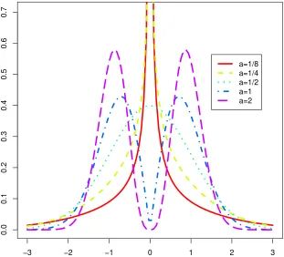
A figure displaying the density (5.10) for different values of a is in appendix. Note that the gaussian density is obtained fora= 1/2. The result was expected because the CS_{-test is based on the QMLE of θ}

0, and the QMLE is obviously efficient in the gaussian case. It can be shown that when the distribution of ηt is of the form (5.10), the MLE does not depend on a. The QMLE is then equal to the MLE, which makes obvious the "if part" of Proposition 5.5. The "only if" part of the proposition shows that there is necessarily an efficiency loss when the test is not based on the MLE of θ0.

This point is illustrated by Figure 1, in which the local asymptotic power of the asymmetry test (in dotted lines) is compared to the optimal asymptotic power given by (5.9). In this figure, the noiseηt is assumed to satisfy a Student distribution with ν > 2 degrees of freedom, standardized in such a way that

Eη2_t = 1. The parameters of the model under the null are α0+ = α0− = 0.2,

β0 = 0.9andδ = 1, which corresponds to a nonstationary model withγ0 = 0.045. In the figure, it can be seen that the local asymptotic power is far from the optimal power whenν is small, but, as expected, the discrepancy decreases asν increases.

6. ESTIMATION WHEN THE POWER δ _{IS UNKNOWN}

In this section, we consider the case where the power δ, now denoted δ0, is unknown and is jointly estimated with θ0. We rewrite the vector of parameters as ζ := (δ, θ′)′, which is assumed to belong to a compact parameter space Υ _⊂ (0,_∞)2 _×[0,∞)3_{. The true parameters value is denoted by ζ}

0 := (δ0, θ′0)′. A QMLE of ζ is defined as any measurable solution ζˆn of

(6.1) ζˆn= (ˆδn,θˆn′)′ =arg min ζ∈Υ

1

n

n

X

t=1

ℓt(ζ), ℓt(ζ) =

ǫ2_t σ2

t(ζ)

+ logσ_t2(ζ),

where

(6.2) σt=σt(ζ) =

ω+α+(ǫ+t−1)δ+α−(−ǫ−t−1)δ+βσtδ−1(ζ)

1/δ

for t = 1, . . . , n (with initial values for ǫ0 and σ0(ζ)). The rescaled residuals are defined by ηˆt =ηt(ˆζn) where ηt(ζ) = ǫt/σt(ζ) for t= 1, . . . , n. For identifiability reasons, we need to slightly reinforce assumption A1 as follows.

A3: The support ofηtcontains at least three points of the same sign, and at least two points of opposite signs.

We also introduce the following technical assumption to handle the derivatives ofℓt with respect to the exponent δ.

A4: _∀ζ_∈Υ,β <_k1/a2₀(η1)kp−1 and k|η1|δlog|η1|kp <∞ for some p >1. For brevity, we only present results for the non stationary cases.

Theorem_6.1. _{Let (1.1)-(1.2) andA3hold. Then, the QMLE defined in (6.1)}

satisfies the following properties.

i) Explosive case. When γ0 >0, ifP(η1 = 0) = 0

(δn,ϑˆ′n)→(δ0, ϑ′0), a.s. as n→ ∞.

If, in addition,κη ∈(1,∞), E|logη21|<∞, ζ0 ∈

◦

Υ, and A4 holds, then

(6.3) √n(ˆδn,ϑˆ′n)−(δ0, ϑ′0)

_{′ d}

→ N n0,(κη−1)I_δ−1

o

,

as n_{→ ∞}, where _Iδ is a positive definite matrix (see LemmaD.4).

ii) At the boundary of the stationarity region. When γ0 = 0, if P(η1 = 0) = 0, and_∀ζ _∈Υ, β <_k1/a0(η1)k−p1 for somep >1,

(δn,ϑˆ′n)→(δ0, ϑ′0), in probability as n→ ∞.

If, in addition, ζ0 ∈

◦

Υ, κη ∈ (1,∞), E|logη12| < ∞ and A2 and A4 are

satisfied, then (6.3) holds.

The presence of parameter δ induces specific difficulties. It turns out that the derivative of the criterion with respect toδ involves the process(∂σ_tδ/∂δ−logσt). A strictly stationary approximation to this process can then be obtained, but in a more complicated way than for the other parameters. To save place, the proofs of this section are given in appendix.

Obviously, stationarity and symmetry tests could be derived as in Sections 4

and 5. Other tests concerning the exponent δ (for instance testing the TARCH model (δ = 1) against the GJR model (δ = 2)) could be considered as well, but we leave this for further investigation.

7. PROOFS AND COMPLEMENTARY RESULTS

7.1 Proof of Proposition 2.1

Writingωt=ω(ξt) and at=a(ξt), we have, for all t >1and 1≤k < t,

(7.1) ht=ωt−1+ k

X

j=1

ωt−j−1 j

Y

i=1

at−i+ht−k−1 k+1_Y

i=1

at−i.

We begin by showing i). Since all the random variables involved in (7.1) are positive,ht≥ωQti=1−1at−i. For any constant ρ > e−γ,we thus have, a.s.

lim inf t→∞

1

tlogρ

t_h

t ≥ logρ+ lim t→∞

1

t

(

logω+ t−1

X

i=1 logai

)

by the ergodic theorem. It follows thatlogρtht, and henceρtht, tend to +∞ a.s asn_{→ ∞}. The second convergence is shown right in the same way, arguing that

E_|logξ2

1|<∞ entails logξt2/t→0a.s. ast→ ∞.

To show ii), first consider the case where h0 = 0. Note that, for all t, the distribution ofht=ht(ξ0, . . . , ξt−1) is equal to that of

(7.2) h∗_t :=ht(ξt, . . . , ξ1) =ω1+ t−1

X

j=1

ωj+1 j

Y

i=1

ai.

Note that, contrary to(ht), the sequence(h∗t)increases with t. The Chung-Fuchs theorem applied to the random walkPt_i=1logaientails thatlim supt→∞

Qt i=1ai = +_∞a.s. It follows thath∗

t →+∞ ast→ ∞. We thus have P(ht≥A) =P(h∗t ≥

A)_→1 for allA >0, from which the first part ofii)easily follows. To prove the first convergence of (2.2), note that the dominated convergence theorem entails

Eψ(ht) =

Z _∞

0 P

n

h∗_t < ψ−1(u)odu→

Z _∞

0 tlim→∞P

n

h∗_t < ψ−1(u)odu= 0.

The second convergence is shown similarly. Now consider the case where the initial value is not equal to zero. It is clear from (7.1), with k = t−1, that ht is an increasing function ofh0. So the convergences to infinity obtained when h0 = 0, and the convergences in (2.2), hold a fortiori when h0 >0. ✷

7.2 Asymptotic behavior of the QMLE of ϑ0

Define the[0,_∞]-valued process

vt(ϑ) =

∞ X

j=1

{α+(η+t−j)δ+α−(−ηt−−j)δ}

a0(ηt−j)

j_Y−1

k=1

β a0(ηt−k)

with the convention Qj_k=1−1 = 1 when j _≤ 1. Let Θ0 = {θ ∈ Θ : β < eγ0} and Θp={θ∈[0,∞)4 :β <k1/a0(η1)k−1

p }.

Lemma _7.1. _{i) When γ0 >0, for any θ∈ Θ0 the process vt(ϑ) is stationary}

and ergodic. Moreover, for any compact Θ∗₀ ⊂Θ0,

sup θ∈Θ∗

0

σδ_t(θ)

ht −

vt(ϑ)

→0 a.s. ast→ ∞.

Finally, for any θ /∈Θ0 it holds that σδt(θ)/ht→ ∞ a.s.

ii) Whenγ0 = 0, for anyθ∈Θp withp≥1, the process vt(ϑ) is stationary and

ergodic. Moreover, for any compact Θ∗

p⊂Θp,

sup θ∈Θ∗ p

σ_tδ(θ)

ht −

vt(ϑ)

→0 in L

p_.

Proof. Assuming, with no generality loss, that σ0(θ) = 0, we have σδt(θ) =

Pt

j=1βj−1zt−j where zt=ω+α+(ǫ+t)δ+α−(−ǫ−t )δ and

σ_tδ(θ)

ht =

t

X

j=1

βj−1

  

j

Y

k=1

ht−k

ht−k+1

  

zt−j

ht−j

.

Noting that

(7.4) ht−k

ht−k+1

= ht−k

ω0+a0(ηt−k)ht−k ≤ 1

a0(ηt−k)

,

the rest of the proof follows from arguments similar to those used in the proof of Lemma A.1 in FZ. Therefore is it omitted. ✷

Lemma _7.2. _{Ifθ∈Θ0, we have vt(ϑ) = 1, a.s. iff ϑ=ϑ0.}

Proof.Straightforward algebra shows that

(7.5) vt(ϑ)a0(ηt−1) =βvt−1(ϑ) +α+(ηt+−1)δ+α−(−ηt−−1)δ.

Hence

{vt(ϑ)−1}a0(ηt−1) =βvt−1(ϑ)−β0+ (α+−α0+)(η+t−1)δ+ (α−−α0−)(−ηt−−1)δ.

It follows thatvt(ϑ) = 1 a.s. iff

β₋β0+ (α+−α0+)(ηt+−1)δ+ (α−−α0−)(−η−t−1)δ= 0.

Thus, if ϑ 6= ϑ0, ηt takes at most two values of different signs, in contradiction with AssumptionA1. The conclusion follows. ✷ Let ω = inf{ω | θ ∈ Θ}, α = inf{α+, α− | θ ∈ Θ}, β = inf{β | θ ∈ Θ},

ω= sup{ω|θ∈Θ},α= sup{α+, α−|θ∈Θ},β= sup{β |θ∈Θ}. Denote by K

any constant whose value is unimportant and can change throughout the proofs. LetΘˇ be the compact set of theϑ’s such that(ω, ϑ′)′ ∈Θ.

Lemma _7.3. _{Suppose that P(ηt= 0) = 0. Then, for any k >0}

Esup ϑ∈Θˇ

1

vt(ϑ)

k

<∞ and Esup θ∈Θ

ht

σδ_t(θ)

!k

<∞.

Proof. Letε > 0 such that p(ε) := P(_|ηt| ≤ ε) ∈[0,1). If |ηt−1|> ε, since the sumvt(ϑ)is greater than its first term, we have,

1

vt(ϑ) ≤

a0(ηt−1)

α+(ηt+−1)δ+α−(−ηt−−1)δ

≤ max(α0+, α0−)

α +

β0

αεδ :=K(ε).

Iterating this method, we can write

sup ϑ∈Θˇ

1

vt(ϑ) ≤

K(ε)

∞ X

i=1

1l_|ηt−1|≤ε. . .1l|ηt−i+1|≤ε1l|ηt−i|>ε

a0(ε)

β

!i−1

.

where a0(ε) = max(α0+, α0−)ǫδ+β0. It follows that, for any integer k,

Esup ϑ∈Θˇ

₁

vt(ϑ)

k

≤ {K(ε)_}k_{1₋p(ε)_}

∞ X

i=1

p(ε)i−1 a0(ε)

β

!k(i−1)

Noting thatlimε→0p(ε) = 0 andlimε→0a0(ε) =β0 we havep(ε)

a0(ε)

β

k

<1for

εsufficiently small. The first result of the lemma is thus proven. Similarly, we have for|ηt−1|> ε,

ht

σδ t(θ)

≤ ω0

ω +

α

α +

β0

αεδ :=H(ε),

and for|ηt−1| ≤εand |ηt−2|> ε,

ht

σδ t(θ) ≤

ω0

ω +

a0(ε)

β H(ε).

More generally,

sup θ∈Θ

ht

σδ t(θ)

≤

∞ X

i=1 1l_|ηt

−1|≤ε. . .1l|ηt−i+1|≤ε1l|ηt−i|>ε

×



ω0

ω

i−2

X

j=0

a0(ε)

β

!j

+ a0(ε)

β

!i−1

H(ε)



.

The conclusion follows by the same arguments as before. ✷

Proof of the consistency results in the cases ii) and iii) of Theorem 3.1. Note that (ˆωn,ϑˆ′n) = arg minθ∈ΘQn(θ), where Qn(θ) =

n−1Pn

t=1{ℓt(θ)−ℓt(θ0)}.We have

Qn(θ) = 1

n

n

X

t=1

η_t2

 



ht

σδ t(θ)

!2/δ −1

 

+ log

σ_tδ(θ)

ht

!2/δ

=On(ϑ) +Rn(θ)

where

On(ϑ) = 1

n

n

X

t=1

η_t2

(

1

v_t2/δ(ϑ) −1

)

+ logv2/δ_t (ϑ)

and

Rn(θ) = 1

n

n

X

t=1

η2_t

 



ht

σδ t(θ)

!2/δ

− 1

v2/δ_t (ϑ)

 

+ log

σδ t(θ)

htvt(ϑ)

!2/δ

.

It suffices to consider the caseθ∈Θ∗₀ whereΘ∗₀ is an arbitrary compact subset of Θ0, because by Lemma7.1i)Qn(θ)→ ∞a.s. if θ /∈Θ0. We have by stationarity and ergodicity ofvt(ϑ), a.s.

lim

n→∞On(ϑ) =E (

1

v₁2/δ(ϑ) −1 + logv 2/δ 1 (ϑ)

)

≥0

becauselogx _≤ x₋1 for x >0.The inequality is strict except when v1(ϑ) = 1 a.s. By Lemma7.2 we thus haveE{On(ϑ)} ≥0, with equality only ifϑ=ϑ0.

By Lemma7.3we prove, as in FZ, that

(7.6) lim n→∞_θsup_∈Θ∗

0

|Rn(θ)|= 0 a.s. (resp. lim n→∞_θsup_∈Θ∗

p

whenγ0 >0(resp.γ0= 0) andΘ∗0,Θ∗pare defined in Lemma7.1, which completes

the proof. ✷

We now need to introduce new[0,∞]-valued processes. Leta(ηt) =α+(η+t )δ+

α₋(₋η_t−)δ_{+β and}

dα+

t =

∞ X

j=1

(η_t+_−j)δ

a0(ηt−j) j_Y−1

k=1

β0

a0(ηt−k)

, dα−_t =

∞ X

j=1

(−η_t−_−j)δ

a0(ηt−j) j_Y−1

k=1

β0

a0(ηt−k)

dβ_t =

∞ X

j=2

(j₋1)_{α0+(ηt+−j)δ+α0−(−ηt−−j)δ}

β0a0(ηt−j)

j−1

Y

k=1

β0

a0(ηt−k)

.

Lemma _7.4. _{Assumeγ0 ≥0 and Eη}4

t <∞. We have

1 √ n n X t=1 ∂ℓt

∂ϑ(θ0)

d

→ N {0,(κη−1)I} asn→ ∞,

where _I= _δ42Ed1d′1 and d′t =

dα+

t , dα−t , dβt

. Moreover, _I is non singular.

Proof.SinceElogβ0/a0(η1)<0, by the Cauchy root test, the processesdαt+, d α− t anddβ_t are stationary and ergodic. Still assuming σ2

0 = 0, we have

∂σδ t

∂(α+, α−)

(θ) = t

X

j=1

βj−1(_{ǫ+_t−j}δ,_{−ǫ−_t−j}δ), ∂σ

2 t

∂β (θ) =

t

X

j=2

(j₋1)βj−2zt−j.

Thus, using a direct extension of (7.4)

1

σδ_t(θ0)

∂σδ t

∂(α+, α−)

(θ0) = t

X

j=1

βj−1

   j Y k=1 σδ t−k(θ0)

σδ_t−k+1(θ0)

 



{(ǫ+_t−j)δ_,(−ǫ−

t−j)δ}

σ_tδ_−j(θ0)

≤ (dα+

t (ϑ0), dα−t (ϑ0)),

1

σδ t(θ0)

∂σδ_t

∂β (θ0) =

t

X

j=2

(j₋1)β₀j−2

   j Y k=1

σδ_t−k(θ0)

σδ

t−k+1(θ0)

  

zt−j

σδ t−j(θ0)

≤ dβ_t(ϑ0),

where the first inequality stands componentwise. Moreover, we have

0_≤dα+

t (ϑ0)− 1

σδ t

∂σδ t

∂α+(θ0)≤st0+rt0,

where

st0 =

t0

X

j=1

(η_t+_−j)δ

a0(ηt−j) j_Y−1

k=1

β0

a0(ηt−k)−

(ǫ+_t−j)δ

β0σtδ−j(θ0) j

Y

k=1

β0σδ_t−k(θ0)

σ_tδ_−k+1(θ0)

,

rt0 =

∞ X

j=t0+1

(η_t+_−j)δ

a0(ηt−j)

j_Y−1

k=1

β0

a0(ηt−k)

For all p ≥ 1, krt0kp → 0 as t0 → ∞ because kβ0/a0(η1)kp < 1 and

k(η₁+)δ/a0(η1)kp <1/α0+. Since, in addition,kβ0σtδ−1(θ0)/σδt(θ0)kp <1, and

β0

a0(ηt−1) −

β0σδt−1(θ0)

σδ t(θ0)

_p =

β0ω0

a0(ηt−1)σtδ(θ0)

_p →0

ast_{→ ∞} by the dominated convergence theorem, st0 =st0(t) converges to 0 in

Lp _{ast → ∞.The same derivations hold true when d}α+

t is replaced by d α− t and

dβ_t. Therefore, dα+

t , d α−

t and dβt have moments of any order, and

(7.7) 1 σδ t

∂σδ_t

∂ϑ (θ0)−dt

→0

inLp for any p≥1.

Using (7.7) and the ergodic theorem, we thus have, asn_{→ ∞},

Var√1

n

n

X

t=1

∂

∂ϑℓt(θ0) =

4

δ2

κη −1

n

n

X

t=1

E(dtd′t) +o(1)→(κη −1)I.

Moreover, it can be shown as in FZ that the Lindeberg condition is satisfied, allowing to apply the Lindeberg central limit theorem for martingale differences (see Billingsley, 1995, p. 476).

Now we show that_I is nonsingular. Suppose there existsx= (x1, x2, x3)′ ∈R3 such that x′Ix= 0. Then we getx′dt= 0, that is,

∞ X

j=1

x1

(η+_t−j)δ

a(ηt−j) +x2

(₋η_t−_−j)δ

a(ηt−j)

+x3(j−1)

α+(η+t−j)δ+α−(−ηt−−j)δ

βa(ηt−j)

!

× j_Y−1

k=1

β a(ηt−k)

= 0, a.s.

It follows that x1(η+_t−1)δ+x2(−ηt−−1)δ =zt−2, a.s. where zt−2 is a measurable function of theηt−j withj >1. Becauseηt−1 is independent ofzt−2, this variable must be a.s. constant. In view of Assumption A1, this entails x1 =x2 = 0and thenx3 = 0.Therefore,I is nonsingular. ✷

Lemma _7.5. _{Let ̟ be an arbitrary compact subset of [0,∞). Assume that}

Elogη2

1 <∞. When γ0 >0 we have, a.s.

∞ X

t=1 sup θ∈Θ0

∂ ∂ωℓt(θ)

< ∞, ∞ X

t=1 sup θ∈Θ0

∂2 ∂ω∂θℓt(θ)

<∞,

sup ω∈̟

1 n n X t=1

∂2ℓt(ω, ϑ0)

∂θi+1∂θj+1 − Iij

= o(1) for all i, j∈ {1,2,3},

1 n n X t=1 sup θ∈Θ

∂3 ∂θi∂θj∂θk

ℓt(θ)

= O(1) for all i, j, k∈ {2,3,4}.

When γ0 = 0 we have, for all i, j, k∈ {2,3,4},

sup ω∈̟

1 n n X t=1

∂2ℓt(ω, α0, β0)

∂θi+1∂θj+1 − Iij

= oP(1),

(7.8) 1 n n X t=1 sup θ∈Θ4

∂3 ∂θi∂θj∂θk

ℓt(θ)

= OP(1).

Proof.This is similar to that of Lemma A.5. in FZ, therefore is it omitted. ✷

Proof of the asymptotic normality in the case ii) of Theorem 3.1. An expansion of the criterion derivative gives

1

√_nPn_{t=1 ∂ω}∂ ℓt(ˆθn) 0

!

= √1

n

n

X

t=1

∂

∂θℓt(θ0) +Jn

√

n(ˆθn−θ0) (7.10)

where _Jn is a 4×4matrix whose elements have the form

Jn(i, j) = 1

n

n

X

t=1

∂2 ∂θi∂θj

ℓt(θ∗i),

where θ_i∗ = (ω∗_i, α∗_i+, α∗_i−, β_i∗)′ is between θˆn and θ0. Moreover, it can be shown that, fori, j= 1,2,3,

(7.11) Jn(i+ 1,1) =o(1/√n), Jn(i+ 1, j+ 1)→ I(i, j) a.s.

The conclusion follows from the last rows of (7.10) and Lemma 7.4. ✷

Proof of the asymptotic normality in the case iii)of Theorem 3.1. Note that (7.10) continues to hold. In view of (7.8)-(7.9), we have

Jn(i+ 1, j+ 1)→ I(i, j) in probability asn→ ∞.

To conclude, by the arguments used in the case ii), it suffices to show that,

(7.12) for i= 2,3,4, E_|Jn(i,1)√n(ˆωn−ω0)| →0 asn→ ∞.

Noting that

(7.13) 1

σδ t(θ)

t

X

j=1

βj−1(ǫ+_t−j)δ_≤ 1

α+

,

andβ₂∗ <1 for nlarge enough, and using the compactness of Θ, we obtain

|Jn(2,1)√n(ˆωn−ω0)|

≤ √K

n

n

X

t=1

2h2/δ_t η2 t

σ2 t(θ2∗)

+ 1

! nPt

j=1(β2∗)j−1(ǫ+t−j)δ

o nPt

j=1(β2∗)j−1

o

σ2δ t (θ2∗)

≤ √K

n

n

X

t=1

2h2/δ_t η_t2 σ2

t(θ2∗) + 1

!

ht

σδ_t(θ₂∗) 1

ht

.

Hence, by Lemma7.3and Hölder’s inequality

E|Jn(2,1)√n(ˆωn−ω0)| ≤

K

√

n

n

X

t=1

E 1

h1+τ_t ,

for anyτ >0.The same bound is obtained when _Jn(2,1) is replaced by Jn(3,1) andJn(4,1). Moreover,

ht=ω0(1 +Zt−1+Zt−1Zt−2+· · ·+Zt−1. . . Z1) +Zt−1. . . Z0σ20.

Hence

1

h1+τ_t ≤

1

ω₀1+τ(1 +Zt−1+Zt−1Zt−2+· · ·+Zt−1. . . Z1)

By AssumptionA2, the conclusion follows. ✷

7.3 Stationarity test

Proof of Theorem4.1.In the stationary caseγ0 <0, standard arguments show that

(7.14) ˆγn=γn(θ0) +

∂γn(θ0)

∂θ′ (ˆθn−θ0) +oP(n−

1/2_),

with

∂γn(θ0)

∂θ = −1 n n X t=1 1

a0(ηt)



  

{a0(ηt)−β0}

1

ht

∂σδ_t(θ0)

∂θ −      0 (η+_t )δ (₋η_t−)δ

1          

= ₋Ψ +oP(1), (7.15)

where Ψ = (1₋ν1)Ω−aand Ω =E∞h1t ∂σδ

t(θ0)

∂θ .Moreover the QMLE satisfies

(7.16) √n(ˆθn−θ0) =−J−1√1

n

n

X

t=1

(1−η2_t) 2

δht

∂σδ_t(θ0)

∂θ +oP(1).

In view of (7.14), (7.15) and (7.16), we have

√

n(ˆγn−γ0) = 1 √ n n X t=1

ut+ Ψ′J−1 1 √ n n X t=1

(1₋η2_t) 2

δht

∂σδ_t(θ0)

∂θ +oP(1).

Note that

Cov √1

n

n

X

t=1

ut, Ψ′J−1 1 √ n n X t=1

(1₋η2_t) 2

δht

∂σδ_t(θ0)

∂θ

!

= 2c

δ Ω′J−

1_Ψ,

where c=Cov(ut,1−ηt2).The Slutsky lemma and the central limit theorem for martingale differences thus entail

√

n(ˆγn−γ0) → Nd

0, σ2_u+ 4c

δΩ

′_J−1_{Ψ + (κ}

η −1)Ψ′J−1Ψ

.

Now letθ0 = (ω0, α0+, α0−,0)′. Noting that θ0′∂σδt(θ0)/∂θ=htalmost surely, we have

E

(

1

ht

∂σδ_t(θ0)

∂θ 1−

1

ht

∂σ_tδ(θ0)

∂θ′ θ0 !)

= 0,

which entails δ₄2Jθ0 = Ωand Ω′J−1Ω = δ

2

4 . It follows that

Ω′_J−1Ψ = (1₋ν1)

δ2

4 −

δ2

4θ0

′_a= δ2

4(1−ν1−α0+ν˜1+−α0−ν˜1−) = 0.

We also have Ψ′J−1_{Ψ =a}′_J−1_{a−(1−ν1)}2_{, which completes the proof of the} asymptotic distribution (4.4) in the case γ0 <0.

Now consider the case γ0 ≥ 0. Let θ∗n be a sequence such that kθn∗ −θ0k ≤ kθˆn−θ0k.By Proposition 2.1(using Assumption A2 when γ0 = 0), we have

1 √ n n X t=1 1 σδ t(θn∗)

∂σδ t(θn∗)

when γ0 > 0 (resp. when γ0 = 0). It can be deduced that, under the same conditions, √n∂2γn(θ∗n)

∂ω∂θ = o(1), and √

n(ˆθ ₋θ0)′∂

2_γ

n(θ∗n)

∂θ∂θ′ (ˆθ−θ0) = o(1), which entails that (7.14) still holds. The previous arguments show that (7.15) holds with

Ω =E

     0

dα+

t (θ0)

dα− t (θ0)

dβ_t(θ0)

    = 1 1₋ν1

     0 ˜ ν1+ ˜

ν1−

ν1/β



  

 and Ψ =

   0 0 0   .

The conclusion follows. ✷

7.4 Asymptotic local powers

Proof of Proposition5.1.The LAN of GARCH models has already been estab-lished in the stationary case (see Drost and Klaassen (1997), Lee and Taniguchi (2005)). The non stationary case will be studied under more general assumptions

in the proof of Proposition5.2. ✷

Proof of Proposition 5.2.Let the functions

g1(y) = 1 +y

f′

f (y) and g2(y) = 1 + 2y f′

f (y) +y

2f′

f

′

(y).

Introduce also the notations

∆1,t(θ) = 1

σt(θ)

∂2σt(θ)

∂θ∂θ′ , ∆2,t(θ) =

1

δ2_σ2δ t (θ)

∂σ_tδ(θ)

∂θ

∂σ_tδ(θ)

∂θ′ .

A Taylor expansion of θn7→Λn,f(θn, θ0)around θ0 yields

(7.17) Λn,f(θn, θ0) =τ′Sn,f(θ0)− 1 2τ

′_In(θ∗

n)τ+Rn, where θ∗

nis between θ0 andθn,

(7.18) Sn,f(θ0) = − 1 √ n n X t=1

g1(ηt) 1

δht

∂σδ_t(θ0)

∂θ ,

I_n(θ) = 1

n n X t=1 g1 _ǫ t

σt(θ)

∆1,t(θ)− 1 n n X t=1 g2 _ǫ t

σt(θ)

∆2,t(θ),

and_Rn is a reminder which is displayed below. As in the proof of Lemma 7.4, it can be seen that

Sn,f(θ0) = − 1

δ√n

n

X

t=1

g1(ηt)dt(ϑ0) +oP(1), dt(ϑ) =

     0

dα+

t

dα−_t dβ_t

    .

Using (5.1), it is easy to see that Eg1(η1) = 0, and thus Eg21(η1) = ιf. The Lindeberg central limit theorem for martingale differences then shows that

Turning to the second term of (7.17) we first note that, similarly to (7.7),

1

ht

∂σδ_t(θ0)

∂θ −dt(ϑ0)

→0 inL

2 _{as t→ ∞.}

Moreover, integrations by parts show that, under (5.1), R y2f′′(y)dy = −2R yf′(y)dy = 2. It follows thatEg2(η1) =−ιf. We thus have, usingEg1(η1) = 0,

In(θ0) = 1

n

n

X

t=1

−g2(ηt)

δ2 dt(ϑ0)d′t(ϑ0) +oPθ₀(1)→If in probability as n→ ∞.

Next, it can be shown that, asn_{→ ∞},

(7.20) _kIn(θn∗)−In(θ0)k →0 in probability.

Finally, we show the convergence in probability to zero of

Rn=υn n

X

t=1

g1(ηt) 1

δht

∂σδ t(θ0)

∂ω −υn

√

nτ′I_n(θ_n∗)e′

1− 1 2nυ

2

ne1In(θ∗n)e′1. Noting that∂σδ_t(θ0)/∂ω is constant and that1/htconverges to 0 inL2 by Propo-sition 2.1, the first term in the right-hand side converges to zero in probability. The two other terms can be handled similarly. The conclusion then follows from

(7.17)–(7.20). ✷

Proof of Proposition 5.3.For simplicity, writeP instead ofPn,0. In the proof of Theorem4.1we have seen that

Tn= 1 √

n

n

X

t=1

ut

σu

+oP(1).

By (5.5) and (7.18), it follows that underP

Tn

Λn,f(θ0+τ/√n, θ0)

!

d −→ N

(

0 −ιf

8τ˜′Iτ˜

!

, 1 c

c ιf 4τ˜′Iτ˜

!)

,

where τ˜′ _{= (τ2, τ3, τ4),c=−}τ′Ed₁(ϑ₀)

δσu Eu1g1(η1) =cf(θ0).Le Cam’s third lemma (seee.g. van der Vaart, 1998, page 90) shows that

Tn−→ Nd (cf(θ0),1), under Pn,τ.

The conclusion easily follows. ✷

Proof of Proposition 5.4. First consider the caseγ0 ≥0. In the proof of (3.4) it has been shown that

√

n( ˆϑn−ϑ0) =−2

δI

−1_√1

n

n

X

t=1

(1−η_t2)dt+oP(1).

Moreover

Λn,f(θ0+τ/√n, θ0) =− 1

δ√n

n

X

t=1

1 +ηt

f′_(ηt)

f(ηt)

˜

τ′_dt−ιf

8τ˜

with τ˜′ _{= (τ2, τ3, τ4). Note also that, since Eη}4

1 < ∞ implies y3f(y) → 0 as |y_{| → ∞}, we have

(7.21) E(1₋η2_t)

1 +ηt

f′_(ηt)

f(ηt)

= 2.

It follows that underPS n,0 √

n( ˆϑn−ϑ0) Λn,f

θ0+ √τ_n, θ0

!

d −→ N

(

03

−ιf 8 τ˜′Iτ˜

!

, (κη −1)I−

1 _τ˜ ˜

τ′ ιf 4τ˜′Iτ˜

!)

.

Le Cam’s third lemma (seee.g.van der Vaart, 1998, page 90) shows that √

n( ˆϑn−ϑ0)−→ Nd

˜

τ_,(κη−1)I−1_{, under P}S

n,τ.

We thus have shown that, in the caseγ0 >0,ϑˆn is a regular estimator of ϑ0, in the sense that√nϑˆn−ϑ0−τ˜/√n

converges to a distribution which does not depend onτ˜_{. More precisely}

(7.22) √nϑˆn−ϑ0−τ˜/√n

_d

−→ N0,(κη −1)I−1

, under P_n,Sτ.

Whenγ0≤0, the same arguments show thatθˆn is a regular estimator ofθ0 √

n(ˆθn−θ0−τ/√n)−→ Nd

0,(κη−1)J−1

, under P_n,Sτ.

In the case γ0 ≤ 0, we thus have (7.22) with I replaced by I∗. Now, noting

that T_nS = e′√n( ˆϑ_n−ϑ₀)

ˆ

σ_TS , and by the same arguments, it follows that T

S n

d −→ N(0,1), under P_n,0S and more generally T_nS _{−→ N}d (cτ,1), under P_n,Sτ, where

cτ = (0,1,−1,0)τ/σ_TS. The conclusion easily follows. ✷

Proof of Proposition 5.5. Recall that we assume γ0 ≥ 0. The case γ0 <0 is obtained similarly, replacing I by I∗. In view of Proposition 5.4 and (5.9), the

CS-test is asymptotically locally UMPU if and only if ce′˜τ =e′τ˜/σ_TS, which is

equivalent to (κη−1)ιf = 4.By Corollary 1 in Francq and Zakoïan (2006), the solutions of this equation are given by (5.10). ✷

8. CONCLUDING REMARKS

Our framework covers the most widely used GARCH models in financial ap-plications. Strictly stationary models are a special case but symmetry tests, and asymptotically valid confidence intervals for the parameters (except the intercept) can be built without this assumption. Surprisingly, while the asymptotic covari-ance matrix of the estimators is sensitive to the stationarity of the underlying process, an estimator which converges to the appropriate covariance matrix in ev-ery situation can be built. Nevertheless, if the interest is on the whole parameter vector, including the intercept, it is important to know whether the observations come from a stationary process or not. To this aim we derived strict stationar-ity/non stationarity tests which are very easy to implement.

volatility, the asymptotic theory derived in this paper can also be established. One key problem, to show consistency, is to find stationary approximations toǫ2_t−j/ht for j = 1,2, . . .. For an ARCH-type model of order q it suffices to take j _≤ q.

Consider standard symmetric GARCH models for simplicity. In the GARCH(1,1) case, the problem can be circumvented because

ǫ2_t−j ht

= ht−1

ht

. . . ht−j ht−j+1

η_t2_−j

can be approximated by a stationary process, in view of

ht−i

ht−i+1 ≈ 1

αη2 t−i+β

for large t.

To have a glimpse of the considerable difficulties encountered when the orders increase, consider a standard ARCH(2) model

ǫt=

p

htηt, ht=ω+α1ǫ2t−1+α2ǫ2t−2.

We have, neglecting ω and for t large enough ht/ǫ2t−1 ≈ Xt and ht/ǫ2t−2 ≈ Yt where

Xt=α1+

α2

Xt−1 1

η_t2₋₁, Yt=α2+α1η

2

t−1Xt−1.

It is not difficult to show that the first stochastic recurrence equation admits a strictly stationary solution (Xt) under mild assumptions on the density of ηt, whatever the values of α1 and α2. From this solution we deduce a strictly sta-tionary solution (Yt) to the second equation. We thus believe that, at least for the consistency, the ARCH(2) model is amenable to a treatment similar to that developed in this paper, but at the price of increasing technical difficulties. To summarize, the ratioht/ht−1 is, for larget, close to i) a constant in the ARCH(1) case, ii) an iid process in the GARCH(1,1) case, iii) the stationary solution of a nonlinear times series model in the ARCH(2) case. Whether or not this ap-proach based on the resolution of nonlinear stochastic recurrence equations could be extended, is left for further investigation.

References

Aknouche, A., Al-Eid, E.M. and A.M. Hmeid (2011) Offline and online weighted least squares estimation of nonstationary power ARCH processes.Statistics and Probability Letters81, 1535–1540.

Aknouche, A. and E.M. Al-Eid (2012) Asymptotic inference of unstable periodic ARCH processes.Statistical Inference for Stochastic Processes15, 61–79.

Aue A., and L. Horváth (2011) Quasi-likelihood Estimation in Stationary and Nonstation-ary Autoregressive Models With Random Coefficients.Statistica Sinica, 21, 973–999.

Berkes, I., Horváth, L. and P.S. Kokoszka (2003) GARCH processes: structure and

esti-mation.Bernoulli9, 201–227.

Billingsley P. (1995)Probability and Measure. John Wiley, New York.

Bougerol, P. and Picard, N. (1992) Strict stationarity of generalized autoregressive

pro-cesses.Annals of Probability20, 1714–1729.

Dickey, D. A. and W. A. Fuller (1979) Distribution of the estimators for autoregressive time series with a unit root. Journal of the American Statistical Association74, 427– 431.

Drost, F. C. and C. A. J. Klaassen (1997) Efficient estimation in semiparametric GARCH

models.Journal of Econometrics81, 193–221.

Drost, F.C., Klaassen, C.A.J. and B.J.M. Werker (1997) Adaptive estimation in time-series models.Annals of Statistics25, 786–817.

Engle, R.F. (1982) Autoregressive conditional heteroskedasticity with estimates of the vari-ance of the United Kingdom inflation.Econometrica50, 987–1007.

Francq, C. and J.M. Zakoïan (2006) On efficient inference in GARCH processes.In: Bertail P, Doukhan P, Soulier P. (eds) Statistics for dependent data. Springer, New-York: 305– 327.

Francq, C. and J-M. Zakoïan (2010) GARCH models: structure, statistical inference and financial applications.Chichester: John Wiley.

Francq, C. and J.M. Zakoïan (2012) Strict stationarity testing and estimation of explosive and stationary GARCH models.Econometrica80, 821–861.

Glosten, L.R., Jaganathan, R. and D. Runkle (1993) On the relation between the ex-pected values and the volatility of the nominal excess return on stocks.Journal of Finance 48, 1779–1801.

Hamadeh, T., and J.M. Zakoïan (2011) Asymptotic properties of LS and QML estimators for a class of nonlinear GARCH Processes.Journal of Statistical Planning and Inference, 141, 488–507.

Higgins, M.L. and A.K. Bera (1992) A class of nonlinear ARCH models.International Eco-nomic Review, 33, 137-158.

Hörmann, S. (2008) Augmented GARCH sequences: dependence structure and asymptotics. Bernoulli14, 543–561.

Hwang, S.Y. and T.Y. Kim (2004) Power transformation and threshold modeling for ARCH innovations with applications to test for ARCH structure.Stochastic Processes and Their Applications110, 295–314.

Karlsen H.A., Myklebust, T. and D. Tjøstheim (2007) Nonparametric estimation in a nonlinear cointegration type model.Annals of Statistics35, 252–299.

Karlsen H.A. and D. Tjøstheim (2001) Nonparametric estimation in null recurrent time series.Annals of Statistics29, 372–416.

Jensen, S.T. and A. Rahbek (2004a) Asymptotic normality of the QMLE estimator of

ARCH in the nonstationary case.Econometrica72, 641–646.

Jensen, S.T. and A. Rahbek (2004b) Asymptotic inference for nonstationary GARCH. Econometric Theory20, 1203–1226.

Klüppelberg, C., Lindner, A. and R. Maller (2004) A continuous time GARCH Process driven by a Lévy process: stationarity and second order behaviour.Journal of Applied Probability41, 601–622.

Lee, S. and M. Taniguchi (2005) Asymptotic theory for ARCH-SM models: LAN and resid-ual empirical processes.Statistica Sinica15, 215–234.

Li, C.W. and W.K. Li (1996) On a double-threshold autoregressive heteroscedastic time se-ries model.Journal of Applied Econometrics11, 253–274.

Ling, S. and D. Li (2008) Asymptotic inference for a nonstationary double AR(1) model.

Biometrika95, 257–263.

Ling, S. and M. McAleer (2003) Adaptative estimation in nonstationary ARMA models with GARCH errors.The Annals of Statistics31, 642–674.

Pan, J., Wang, H., and H. Tong (2008) Estimation and tests for power-transformed and

threshold GARCH models.Journal of Econometrics, 142, 352-378.

Phillips, P.C.B. and P. Perron (1988) Testing for a Unit Root in Time Series Regression Biometrika, 75, 335–346.

Rabemananjara, R. and J-M. Zakoïan (1993) Threshold ARCH Models and Asymmetries in Volatility.Journal of Applied Econometrics8, 31–49.

van der Vaart, A.W. (1998) Asymptotic statistics. Cambridge University Press, United Kingdom.

Appendices

APPENDIX A: DENSITIES ENSURING LOCAL OPTIMALITY OF THE ASYMMETRY TEST

Figure2shows densities (5.10) for different values ofa. For such densities, the test (4.7) is asymptotically locally UMPU for the testing problem (4.6).

APPENDIX B: NUMERICAL ILLUSTRATIONS

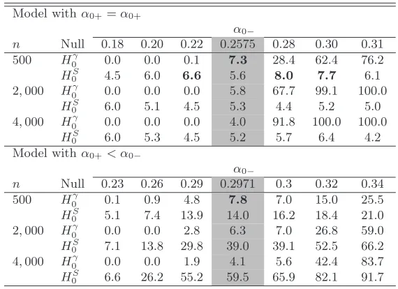
We first simulated N = 1,000 independent trajectories of size n = 500, n = 2,000 and n = 4,000 of an asymmetric GARCH(1,1) model, with a parameter of the form θ0 = (0.1, α0+, α0−,0.8) and the standardized Student distribution

with 7 degrees of freedom for ηt. With such parameters, we have γ0 = 0 for

α0+ =α0− = 0.2575 or forα0+ = 0.22 and α0−= 0.2971, in particular. Table 1

studies the finite sample properties of the stationarity and asymmetry tests based respectively on the statistics Tn and TnS. The first rows of the table concern tests applied to a symmetric model α0+ = α0−, and the last rows concern the

asymmetric model.

The empirical size of a test of theoretical level α = 5%, over N = 1,000 independent replications of the null hypothesis, belongs to the interval [3.6%, 6.4%] with probability 95%. In view of this basic result, one can consider that the error of first kind of the asymmetry test is well controlled. Indeed, except for three values ofα0−whenn= 500(displayed in bold-face in the table), in the first

part of Table 1 the relative frequency of rejection of H₀S is always between the significance bounds 3.6% and 6.4%, regardless of the value of γ0. The empirical frequency of rejection of the stationarity test under the null, displayed in the rows

H₀γ of the two gray columns, is also quite satisfactory when n >500. Looking at the second part of Table 1, one can note that the asymmetry test behaves as expected under the alternative. Indeed the frequency of rejection ofHS

0 increases when α0− moves away from α0+ = 0.22 and when the sample size n increases. As expected from the asymptotic study, as n_{→ ∞}, the frequency of rejection of

H₀γ tends to zero whenγ0 <0(on the left of the gray columns) and tends to one whenγ0>0(on the right of the gray columns).