http://www.scirp.org/journal/jis ISSN Online: 2153-1242
ISSN Print: 2153-1234
Cyber Security: Nonlinear Stochastic Models for
Predicting the Exploitability
Sasith M. Rajasooriya
*, Chris. P. Tsokos, Pubudu Kalpani Kaluarachchi
Department of Mathematics and Statistics, University Of South Florida, Tampa, Florida, USA
Abstract
Obtaining complete information regarding discovered vulnerabilities looks extremely difficult. Yet, developing statistical models requires a great deal of such complete information about the vulnerabilities. In our previous studies, we introduced a new concept of “Risk Factor” of vulnerability which was cal-culated as a function of time. We introduced the use of Markovian approach to estimate the probability of a particular vulnerability being at a particular “state” of the vulnerability life cycle. In this study, we further develop our models, use available data sources in a probabilistic foundation to enhance the reliability and also introduce some useful new modeling strategies for vulne-rability risk estimation. Finally, we present a new set of Non-Linear Statistical Models that can be used in estimating the probability of being exploited as a function of time. Our study is based on the typical security system and vulne-rability data that are available. However, our methodology and system struc-ture can be applied to a specific security system by any software engineer and using their own vulnerabilities to obtain their probability of being exploited as a function of time. This information is very important to a company’s security system in its strategic plan to monitor and improve its process for not being exploited.
Keywords
Vulnerability Lifecycle, Stochastic Modeling, Security Risk Factor, Markov Process, Risk Evaluation
1. Introduction
“Risk” is an unavoidable phenomenon in the Cyber world. Information systems ranging from very small and personal level apps to massive corporate and gov-ernment applications and system platforms are facing the threat from Cyber-at- tacks [1] in various dimensions. The number of such attacks and the magnitude
How to cite this paper: Rajasooriya, S.M., Tsokos, C.P. and Kaluarachchi, P.K. (2017) Cyber Security: Nonlinear Stochastic Mod-els for Predicting the Exploitability. Journal of Information Security, 8, 125-140.
http://dx.doi.org/10.4236/jis.2017.82009
Received: March 22 2017 Accepted: April 27, 2017 Published: April 30, 2017
Copyright © 2017 by authors and Scientific Research Publishing Inc. This work is licensed under the Creative Commons Attribution
International (CC BY 4.0).
http://creativecommons.org/licenses/by/4.0/
of the hazards have been heavily increasing throughout recent years. Hackers are getting more active and effective. The risk is getting higher. System administra-tors and defending professionals are working hard to understand attackers, at-tacking strategies and effectively defend atat-tacking attempts. To establish suc-cessful defending platforms, a proper understanding of the “risk” associated with a given vulnerability [2] [3] is required. If we have effective models that enable the defenders and system administrators to successfully predict the risk of a giv-en vulnerability being exploited as a function of time, it will be helpful to plan and implement security measures, allocate relevant resources and defend the systems accordingly. We, in this study, improve the Markovian approach of Vulnerability Life Cycle Analysis [2] to come up with better modelling tech-niques to evaluate the “risk factor” using probability and statistical methods.
The objective of this study is to propose and present a rational set of methods to identify the probabilities for each different state in the vulnerability life cycle [2][4] [5] and use this information to develop three different statistical models to evaluate the “Risk Factor” [2] [5] of a particular vulnerability at time “t”. In our recent study “Stochastic Modelling of Vulnerability Life Cycle and Security Risk Evaluation” (Journal of Information Security, 7, 269-279) [2], we intro-duced the strategy of using Markov processes to obtain the “transition proba-bility matrix” of all the states of a particular vulneraproba-bility as a function of time. We iterated the Markov process and determined that it reached the “steady state” with probabilities of reaching the “absorbing states” [1] [2]. The two ab-sorbing states were identified as “exploited” and “patched” states. We pro-ceeded to introduce the “Risk Factor” that could be used as an index of the risk of the vulnerability being exploited [1]-[7]. Finally, we presented successful sta-tistical models that could calculate the “Risk Factor” more conveniently without going through the Markovian process [1] [2] [6].
However, in this process, we used a logical and realistic approach to assign in-itial probabilities for each state of the vulnerability. In this study, we introduce more relevant and sophisticated sets of methods to assign the initial probabilities for each state of Vulnerability Life Cycle based on several logical assumptions. We use the CVSS score [3] [8] as we did earlier, but here we calculate and in-troduce initial probabilities taking the entire CVE Data Base
(http://www.cvedetails.com/) into consideration.
Finally, using our new methods, we develop three new statistical models for vulnerabilities that differ based on their vulnerability score ranging from 0 to 10 as low risk (0 - 3.9), medium risk (4 - 6.9) and high risk (7 - 10). Using these models the user will be able to estimate the “Risk” of a particular vulnerability being exploited at time “t” and to observe the expected behavior of the vulnera-bility throughout its life cycle.
1.1. Vulnerability Life Cycle Analysis Method
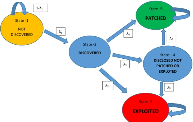
Vul-nerability Life Cycle. The VulVul-nerability Life Cycle Graph that we discussed is presented below by “Figure 1”. When we draw a Life Cycle Graph for a given vulnerability, it has several nodes which represent the stages of the Vulnerability Life Cycle. Earlier we assigned logical probabilities for a hacker to reach each state by examining the properties of a specific vulnerability. Life Cycle Graph has two absorbing states [2] [4] [5] [6] that are named “Patched” state [2] [4] [5] [6] [7] and “Exploited” state [1] [2] [4] [5] [6] [7]. Therefore, this allowed us to model the Life Cycle Graph as an absorbing Markov chain. It should be noted that in the figure below the states three and five are absorbing states of this Life Cycle Graph as there are no out flaws from those states.
We define, λi to be the probability of transferring from state i to state j. Where,
i j
,
=
1, 2, 3, 4, 5.
In actual situations the probability of discovering a vulnerability can be as-sumed very small. Therefore, for λ1 we had assigned a small value. Then prob-abilities for λ λ λ λ2, 3, 4, 5, were also assigned accordingly. Then we checked sev-eral random values for λis and observed the behavior of each different state to be a function of time.
Using these transition probabilities we could derive the absorbing transition probability matrix for a Life Cycle of a particular Vulnerability, which follows the properties defined under Markov Chain Transformation Probability Method [2].
[image:3.595.210.538.500.708.2]However, in our present study, instead of randomly assigning transition probabilities for each of the state presented in the Life Cycle, we use a new set of methods that are probabilistically more reliable. It is challenging to acquire a complete set of information relevant to Vulnerabilities in a manner that we can calculate the required probabilities conveniently. Therefore, we use available and
reliable data resources about Vulnerabilities to develop our methodology that we discuss in the section that follows.
1.2. Common Vulnerability Scoring System (CVSS) and Common
Vulnerabilities and Exposures (CVE)
It is important to discuss here the usage of Common Vulnerability Scoring Sys-tem (CVSS) [8] and CVE Details [9], as we gather data from those resources. Common Vulnerability Scoring System (CVSS) is the commonly used and freely available standard for assessing the magnitude of Information System Vulnera-bilities. CVSS gives a score for each vulnerability scaling from 0 to 10 based on several factors. National Vulnerability Database (NVD) [3] provides CVSS score and updates continuously as new vulnerabilities are discovered. CVSS score is calculated using three main matrices named, Base Matric, Temporal Metric and Environmental Metric. However, NVD data base provides us with the Base Me-tric Scores for the Vulnerability only because the Temporal and Environmental Scores are varied on other factors related to the organization that uses the com-puter system. The Base score for more than 75,000 different vulnerabilities are calculated using 6 different Matrices. It is managed by the Forum of Incident Response and Security Teams (FIRST). CVSS establishes a standard measure of how much concern vulnerability warrants, compared to other vulnerabilities, so that efforts can be prioritized. The scores range from 0 to 10. Vulnerabilities with a base score in the range 7.0 - 10.0 are High, those in the ranges 4.0 - 6.9 are Medium, and 0 - 3.9 are Low. Hence, the three transition probability matrices and statistical models that we develop in this study are based on this classifica-tion of the CVSS score.
Common Vulnerabilities and Exposures (CVE) is a dictionary resource and CVE Detail website [9] provides us with the data base in the basic categories with different CVSS scores. CVE Details provide us with quantities of vulnera-bilities in different levels of magnitudes ranging from 0 to 10. Instead of ran-domly assigning a reasonable probability for each different states (λis), we now use these data resources as per their availability in estimating probabilistically reliable values for each state. Our approach in assigning initial probabilities into each state of the Life Cycle is discussed in the subsection 2.2 below.
2. Methodology
2.1. Methodology of Assigning Initial Probabilities
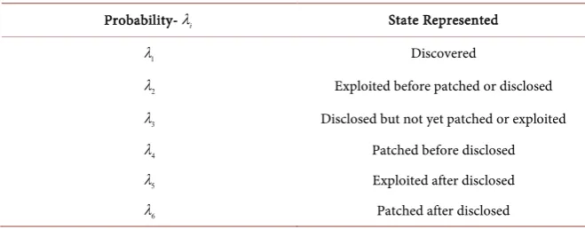
Table 1. States Represented by the Transition Probabilities in the Vulnerability Life Cycle.
Probability-λi State Represented
1
λ Discovered
2
λ Exploited before patched or disclosed
3
λ Disclosed but not yet patched or exploited
4
λ Patched before disclosed
5
λ Exploited after disclosed
6
λ Patched after disclosed
under each CVSS score level.
We start with the CVSS scores available for each vulnerability and categorize them and take the counts for the three different levels of vulnerabilities for possible states. However, it should be noted that, there are no data resources available providing all the data requirements here we have. Therefore, when the CVSS classifications available in the CVE detail website satisfy our requirements, we use those data and when they are not sufficient to make a reliable estimate we use information given by “Stefan Frei” in his thesis [4] and “Secunia Vulnerabil-ity information report” [10].
We categorized 75,705 vulnerabilities according to their CVSS score and un-der each of the three categories to find out number of total vulnerabilities and number of exploitations. We shall use this information to assign probabilities of discovery (λ1) and exploitability (λ2) for each CVSS score level.
To assign probabilities for Disclosed but not yet patched or exploited (λ3), Patched before disclosed (λ4), exploited after disclosed (λ5) and patched after disclosed (λ6) we used Secunia vulnerability report information [10] and Frei’s results given in his study [4].
2.2. Estimating
λ
12.3. Assumptions Made for
λ
1When calculating λ1, it was assumed that, the number of unknown vulnerabili-ties in a particular year are discovered in the next year and the accumulated number of vulnerabilities in a particular year is an estimate for the population size of the vulnerabilities in the previous year.
2.4. Estimating
λ
2Estimate for λ2, “the probability of a particular vulnerability being exploited [13][14] before patched or disclosed” was calculated using the data provided in the CVE Detail website. The entire set of exploited vulnerabilities were calcu-lated for 10 different categories (or CVSS score levels) of interest.
2.5. Estimating
λ
3,
λ
4,
λ
5and
λ
63
λ , “the probability of a vulnerability being disclosed but not yet patched or ex-ploited” is calculated using the equation, λ3= −1
(
λ2+λ4)
.For λ4, “the probability of a vulnerability being patched before disclosed”, we used information available in “Secunia Report on Vulnerability”.
To estimate λ5, “probability of a vulnerability being exploited after disclosed” and λ6, “probability of a vulnerability being patched after disclosed” we used in-formation given by “Stefan Frei” in his doctoral thesis [4]. Frei, estimates that the probability of a vulnerability being exploited after it is disclosed is greater than the probability of it being patched. He estimates that there is a probability around 0.6, for a disclosed vulnerability being exploited. Therefore, we, in developing our model used, fix values of 0.6 and 0.4 respectively for λ5 and λ6.
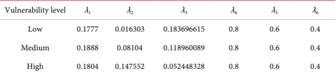
“Table 2” below presents our results on probabilities for each state with re-spect to each category/level of vulnerability.
Using these transition probabilities for each level we can now derive the ab-sorbing transition probability matrix for a Vulnerability Life Cycle, which fol-lows the properties defined under Markov Chain Transformation Probability Method [15] [16] [17] [18] [19].
2.6. Transition Matrix for Vulnerability Life Cycle
[image:6.595.207.539.656.730.2]2.6.1. Executing the Markov Process to Transition Probability matrix Now that we have the Vulnerability Life Cycle Graph with two absorbing states and initial probability estimates for each state, we can write the general form of the transition probability matrix [15] [16] [19] for vulnerability life cycle as follows.
Table 2. Estimates of Transition Probabilities for each Category of Vulnerabilities.
Vulnerability level λ1 λ2 λ3 λ4 λ5 λ6
1 1
2 3 4
5 6
0 0 0
0 0
0 0 1 0 0
0 0 0
0 0 0 0 1
1
P
λ λ
λ λ λ
λ λ = − where,
( )
iP t -Probability that the system is in state i at time t. For t=0 we have:
( )
1 0 1
P = , Probability that the system is in State 1 at the beginning (t=0).
( )
2 0 0
P = , P3
( )
0 =0, P4( )
0 =0, P5( )
0 =0.Therefore, the initial probability can be given as
[
1 0 0 0 0]
, that is, the probabilities of each state of the Vulnerability Life Cycle initially. It is clear that, the “State 1” (Not Discovered) with probability of one represents that at the ini-tial time (for t=0), where the Vulnerability has not yet been discovered and therefore the probabilities for all others stages are zero.Now, for three different categories of Vulnerabilities, we can iterate the transi-tion probability matrix using Markovian process [15] until the matrix reaches its “steady state”. The iteration algorithm is explained below.
For t=0, we have
( )0
[
]
1 0 0 0 0 .
P =
For t=1 , results in
( )1 ( )0
P =P P
. For t=2, we can write
( )2 ( ) ( )0 2
P =P P
. And thus, for = n , we have
( )n ( ) ( )0 n
P =P P
.
Using this method, we can now find the probability that is changing with time and is related to each “state” and then proceed to find the statistical model that can fit the vulnerability life cycle.
As an example, for the vulnerabilities in Category one, where λ =1 0.1777,
2 0.0163
λ = , λ =3 0.1837 , λ =4 0.8 , λ =5 0.6 , λ =6 0.4 the transition probability matrix is written as follows:
0 0 0
0 0 0.8
0 0 1 0 0
0
0.8223 0.1777
0.0163 0.1837
0.6 0.4
0 0
0 0 0 0 1
P =
that is, the minimum number of steps so that the vulnerability reaches its sorbing states is 86 and the resulting vector of probabilities for each of the ab-sorbing states is obtained as the output of the calculation process. As shown be-low, the transition probabilities are completely absorbed into the two absorbing states which gives the “probability of the vulnerability being exploited” and the “probability of the vulnerability will be patched”. All other states have reached the probability of zero. That is,
0 0 0
0 0 0.8
0 0 1 0 0
0
0.8223 0.1777
0.0163 0.1837
0.6 0.4
0 0
0 0 0 0 1
P =
( )86
0.1524 0 0.8476 0 0 0.1524 0.8476
,
0 0 1 0 0
0 0 0
0 0 0
0 0 0 0.6 0.4 0 1 P ⇒ =
( )86 ( ) ( )0 86
[
]
0 0 0.1265 0 0.8735 .
P =P P =
That is, it will take the hacker 86 steps and a 12.7% chance to exploit the secu-rity system and 87.3% probability to reach the patched state. Thus we are sure that after t=86, one of the two states will be reached.
Initially, we defined the 3rd state as “the state of being exploited” and the 5th state as “the state of being patched” in the vulnerability life cycle. Based on the current data resources available relevant to the vulnerabilities of category one we can use these results as estimates for the probabilities of being exploited and be-ing patched. The results from this Markovian model [15] for the vulnerability life cycle show that the sum of the resulting probabilities equals to one (0.1265 + 0.8735 = 1). This in other words indicates that our model estimates that one of these results are expected after t=86 (ex: after 86 days) for a vulnerability in category one. Hence, it is clear that once the “steady state” is achieved, for a vul-nerability of category one, estimates of the probability of being exploited is 12.65% and the probability of being patched is 87.35%.
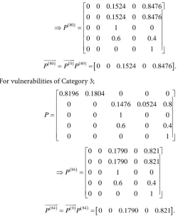
Similarly, for vulnerabilities of categories two and three, the transition proba-bility matrices can be obtained. Transition probaproba-bility matrices and resulting steady state vectors for those categories are given below.
For vulnerabilities of Category 2;
0 0 0
0 0 0.8
0 0 1 0 0
0 0
0.8112 0.1888
0.081 0.119
0.6 0
0 0 1
( )80
0.1524 0 0.8476 0 0 0.1524 0.8476
0 0 1 0 0
0 0 0
0 0 0 0 0 0.6 0 0 .4 0 1 P ⇒ =
( )80 ( ) ( )0 80
[
]
0 0 0.1524 0 0.8476 .
P =P P =
For vulnerabilities of Category 3;
0 0 0
0 0 0.8
0 0 1 0 0
0
0.8196 0.1804
0.1476 0.0524
0.6 0.4
0 0
0 0 0 0 1
P =
( )84
0.1790 0 0.821 0 0 0.1790 0.821
0 0 1 0 0
0 0 0
0 0 0 0 0 0.6 0 0 .4 0 1 P ⇒ =
( )84 ( ) ( )0 84
[
]
0 0 0.1790 0 0.821 .
P =P P =
“Table 3” below summarizes our results. Number of iterations (steps) that it takes to reach the “steady states” and resulting row vectors of probabilities for each three categories of vulnerabilities are given in this table.
2.6.2. “Risk Factor”—Calculating the Risk as a Function of Time
Now that we have the steady state vector with the probabilities for patching and getting exploited, we can calculate the risk of a particular vulnerability using the“risk factor”. In our previous study [2] we have introduced this risk factor as follows.
( )
(
)
( )
Risk v ti =Pr viis in state 3 at time t ×Exploitability score vi
[image:9.595.218.469.70.378.2]Exploitability score [3] for the vulnerability can be taken from the CVSS score as we mentioned earlier. With our results for three different levels of vulnerabili-ties, now we have a better index for the risk factor since our initial probabilities were not just chosen randomly, but were estimated using the available and relia-ble data sources. As an example, let’s consider a vulnerability in the lower level
Table 3. Number of iterations (steps) to reach the steady state and Steady State Vector for each category of Vulnerability.
Category Number of iterations Steady state being exploited Probability of being patched Sum Probability of
with an exploitability score of 2.4. Assume that we need to find the Risk factor of that vulnerability at t=50. Then, using the Markov process we can come up with the resulting vector of the vulnerability that gives us the probabilities of be-ing in each different state at that particular time. However, iteratbe-ing Markov process for each time would not be a very efficient process due to the analytical calculations. Therefore, we proceed to move on to develop three different nonli-near statistical models that make it much more convenient for the designed cal-culation.
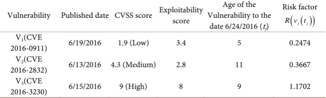
To further explain the usage of the Risk Factor let’s take an example. Consider a vulnerability given in Table 4. With the published date and the exploitability score known for that vulnerability, we can now calculate the risk of being ex-ploited at a particular date from the published date. For the first vulnerability V1 (CVE 2016-0911) which is a low risk vulnerability the risk factor is 0.2474 and for the other two categories of medium and high risk levels, vulnerabilities V2(CVE 2016-2832) and V3(CVE 2016-3230), risk factors are 0.3667 and 1.17702 respectively.
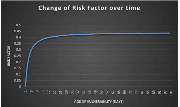
The risk factor can be graphed as a function of time. The figure below shows the behavior of the risk factor of the middle level vulnerability V2(CVE 2016-2832) over a time period of 101 days starting from 6/13/2016. We notice that the risk factor increases rapidly within around first 10 days indicating that once a vulnerability is published, the risk of being exploited rapidly increases. Even after this rapid increase, the risk does not show a decreasing behavior. This specific behavior is due to our model structure of the vulnerability life cycle. That is, consisting with two absorbing states (being exploited and being patched), we assume that either one of two outcomes are possible for a given vulnerability. Therefore, considering state of being exploited as an absorbing state the life cycle does not move to any other state beyond being exploited which explains why this graph stay increased without decreasing over the time.
[image:10.595.210.539.627.726.2]Figure 2 above illustrates the behavior of the Risk Factor as a function of time. The curve shows a rapid increase in the risk factor initially as expectable since the vulnerability immediately create a risk with its discovery and disclosure. Based on the graph, we can conclude that over the time with a life cycle consist-ing two absorbconsist-ing states, the Risk Factor of a given vulnerability increases rapid-ly and become stable at a higher level of risk without decreasing back. This be-
Table 4. Three vulnerabilities in each categories with their details and the calculated risk factors.
Vulnerability Published date CVSS score Exploitability score Vulnerability to the Age of the date 6/24/2016 (tj)
Risk factor
( )
(
j j)
R v t
V1(CVE
2016-0911) 6/19/2016 1.9 (Low) 3.4 5 0.2474 V2(CVE
2016-2832) 6/13/2016 4.3 (Medium) 2.8 11 0.3667 V3(CVE
havior exemplifies the threat any vulnerability would impose on an information system. As far as a proper patch is released and installed a probable harm from a given vulnerability increases monotonously. However, it should not be misin-terpreted in the view point that the risk from a given vulnerability never reduces. Our Absorbing Markovian Model does not consider some of the interactions that might take place in the real world situations. Our intention here is to show the impact of a vulnerability until it is not patched. Outcomes from the situa-tions where patching attempts and exploit attempts after and before disclose should be explained in much border modeling aspect of the vulnerability life cycle.
3. Nonlinear Statistical Models for Exploitability
3.1. Model Building
In the previous section we developed an analytical algorithm that identifies the number of steps (time) that the transition probability matrix of the vulnerability life cycle will reach a steady state. Thus, for a given vulnerability in the categories of Low, Medium and High risk levels, we can include with the probability of be-ing exploited (havbe-ing hacked) and the probability of bebe-ing patched as a function of time. However, this process is time consuming and the Markovian iteration process [1] [2] [15] [16] would be quite difficult to perform every time. Using this approach to find the minimum number of steps for each category we ob-tained t = 86 steps for category one vulnerabilities, t = 80 steps for category two vulnerabilities and t = 84 steps for category three vulnerabilities. Then, we rec- orded the probability of being exploited at the each step. Thus, we have for each category a 2 × 86, 2 × 80 and 2 × 84, matrices of information, respectively. Our goal is to utilize this information and develop a statistical model for each cate-gory to be able to predict the probability of being exploited as a function of time and thus bypassing the analytical difficulties.
[image:11.595.217.533.526.713.2]A sample of the data for each category is shown in Appendix A. All these of
Figure 2. Behavior of the Risk Factor as a function of time. 0
0.05 0.1 0.15 0.2 0.25 0.3 0.35 0.4 0.45 0.5
1 5 9 13 17 21 25 29 33 37 41 45 49 53 57 61 65 69 73 77 81 85 89 93 97
101
RI
SK
F
AC
TOR
AGE OF VULNERABILITY (DAYS)
the data sets exhibit nonlinear behavior and thus multiple regression is not ap-plicable. After very exhaustive research, we were able to identify two sets of non-linear statistical models for each category.
The general analytical focus of the statistical models that we found is of the forms:
Model 1: Y (exploitation probability) = 0 1 2
1 lnt t
α +α +α +ε and
Model 2: Y (exploitation probability) = 0 1 2
1
ln(ln )t t
β +β +β +ε,
where, Y is the probability of being exploited, α and
β
are the vector of coef-ficients or weights, t being the time given in steps and ε is the modelling error. We used the method of maximum Likelihood estimation to obtain the es-timates of the coefficients that drives these models.Model-1
The best nonlinear statistical model that we developed for Low, Medium and High Vulnerability categories are given below along with their R2 (coefficient of determination), 2
adj
R (R2 adjusted).
Low (Category one) risk vulnerabilities:
( )
1
0.084197 0.116756 0.011321ln ,
Y t
t
= − +
with R2 =0.8684, 2 0.8653.
adj
R =
Medium (Category two) risk vulnerabilities:
( )
1
0.111073 0.143992 0.011461ln ,
Y t
t
= − +
with R2 =0.8888, 2 0.8859.
adj
R =
High (Category three) risk vulnerabilities:
( )
1
0.133927 0.169314 0.012375 ln ,
Y t
t
= − +
with 2
0.8988,
R = Radj2 =0.8963.
As we will discuss R2 reflects on the quality of the proposed model. Model-2
In investigating to see if we can improve the precision of the Model 1, we have found that by implementing another logarithmic filter to our initial model to further homogenizing the variance of our data. We obtained a set of models that gives us better results increasing the accuracy of our prediction approximately by 9% compared to the Model 1. New model equations for each of the categories are given below.
Low (Category one) risk vulnerabilities:
( )
(
)
1
0.135441 0.308532 0.002030 ln ln
Y t
t
= − +
with R2 =0.9576, 2 0.9566.
adj
R =
Medium (Category two) risk vulnerabilities:
( )
(
)
1
0.169518 0.356821 0.007011ln ln
Y t
t
= − +
with R2 =0.962, 2 0.961.
adj
R =
High (Category three) risk vulnerabilities:
( )
(
)
1
0.135441 0.308532 0.002030 ln ln
Y t
t
= − +
with 2
0.9588,
R = Radj2 =0.9577.
Thus, Model 2 is a significant improvement in the R2 over model 1.
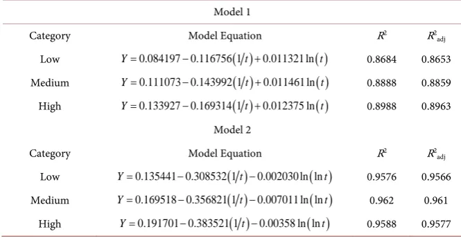
Both models give very good predictions of the probability of exploitation as a function of time. However, “Model-2” seems to give better predictions because of the additional logarithmic filtering that we applied to homogenize the va-riance further. Table 5 summarizes the 6 model equations with respective R2 (coefficient of determination), 2
adj
R (R2 adjusted) values for convenient
com-parison.
3.2. Evaluation of the Models
We used R2 (coefficient of determination), 2
adj
R (R2 adjusted) and residual
anal-ysis using actual data that we did not use in the model building to validate the accuracy and the quality of these models. R2 is commonly used to measure the goodness of a statistical model and is defined as,
2
1 ,
Reg Res
Total Total
SS SS
R
SS SS
= = −
where SSRes or SSE is the Sum of Squares of Residual and SSTotal is the Total Sum of Squares. It is also referred to as the Coefficient of Determination. In our case the 2
0.96
R = states that the model is an excellent fit such that the 96% of the behavior in the response variable (probability of being exploited) is ex-plained and predicted by the attributable variable (time-t) and only a 4% of the change in the response variable is not explained due to the variance.
In order to be more confident in interpreting the value of R2 we also calculate the 2
adj
R (R2 adjusted) to address the issue of bias. 2
adj
[image:13.595.205.538.566.738.2]R (R2 adjusted) is defined by
Table 5. New Nonlinear Statistical Models to estimate the probability of being exploited as a function of time.
Model 1
Category Model Equation R2 R2
adj
Low Y=0.084197 0.116756 1−
( )
t +0.011321 ln( )
t 0.8684 0.8653Medium Y=0.111073 0.143992 1−
( )
t +0.011461 ln( )
t 0.8888 0.8859High Y=0.133927 0.169314 1−
( )
t +0.012375 ln( )
t 0.8988 0.8963Model 2
Category Model Equation R2 R2
adj
Low Y=0.135441 0.308532 1−
( )
t −0.002030 ln ln( )
t 0.9576 0.9566Medium Y=0.169518 0.356821 1−
( )
t −0.007011 ln ln( )
t 0.962 0.961(
)
(
)
2 1
1 Res
adj
Total
n SS
R
n p SS
− = −
− ,
where, n is the sample size and, p is the number of risk factors (attributable va-riables) in our models. The closer the R2 and 2
adj
R to one, the higher the quality
of our models.
We also performed residual analysis of all the models to determine if the error factor has significantly contributed to the accuracy of our models. In all cases, the residual error was not significant. Finally we tested all our models with the actual data that we did not include in developing the models and the results were exceptional.
As mentioned, we needed a best fitting three Statistical models to calculate the “risk factor” conveniently. In other words, we expected to obtain a best fitting model that can replace the Markovian iteration and hence to avoid the difficulty in estimating of the probabilities for time “t” earlier to the “steady state”. With these new models we have achieved our goal.
4. Conclusion
In this study, we continue to improve the models we build up in our previous study [2]. We have improved the calculation methods of initial probabilities and created the Transition Probability Matrix in using of the Markovian process that we introduced in our previous studies. We used CVSS data presented in CVE details website and calculated initial probabilities for discovering and exploiting a vulnerability based on the records on last 17 years data. Finally, we created two sets of three models for predicting the risk of a particular vulnerability being ex-ploited as a function of time. The models we presented are proven to have an excellent fit with the Markovian process probabilities. Therefore, we can replace the Markovian process using these models since these models enable us to get rid of analytical requirement to execute the Markovian iteration process of iden-tifying the steady states of being exploited or being patched for each vulnerabili-ty.
References
[1] Kaluarachchi, P.K., Tsokos, C.P. and Rajasooriya, S.M. (2016) Cybersecurity: A Sta-tistical Predictive Model for the Expected Path Length. Journal of Information Secu- rity, 7, 112-128. https://doi.org/10.4236/jis.2016.73008
[2] Rajasooriya, S.M., Tsokos, C.P. and Kaluarachchi, P.K. (2016) Stochastic Modelling of Vulnerability Life Cycle and Security Risk Evaluation. Journal of information Se- curity, 7, 269-279. https://doi.org/10.4236/jis.2016.74022
[3] NVD. National Vulnerability Database. http://nvd.nist.gov/
[4] Frei, S. (2009) Security Econometrics: The Dynamics of (IN) Security. PhD Disser-tation, ETH, Zurich.
[6] Kijsanayothin, P. (2010) Network Security Modeling with Intelligent and Complex-ity Analysis. PhD Dissertation, Texas Tech UniversComplex-ity, Lubbock, TX.
[7] Alhazmi, O.H., Malaiya, Y.K. and Ray, I. (2007) Measuring, Analyzing and Predict-ing Security Vulnerabilities in Software Systems. Computers & Security, 26, 219- 228. https://doi.org/10.1016/j.cose.2006.10.002
[8] Schiffman, M. Common Vulnerability Scoring System (CVSS).
http://www.first.org/cvss/
[9] CVE Details. http://www.cvedetails.com/
[10] Secunia Vulnerability Review 2015: Key Figures and Facts from a Global Informa-tion Security Perspective. March 2015.
https://secunia.com/?action=fetch&filename=secunia_vulnerability_review_2015_p df.pdf
[11] Alhazmi, O.H. and Malaiya, Y.K. (2008) Application of Vulnerability Discovery Models to Major Operating Systems. IEEE Transactions on Reliability, 57, 14-22. https://doi.org/10.1109/TR.2008.916872
[12] Alhazmi, O.H. and Malaiya, Y.K. (2005) Modeling the Vulnerability Discovery Pro- cess. Proceedings of 16th International Symposium on Software Reliability Engi-neering, Chicago, 8-11 November 2005, 129-138.
https://doi.org/10.1109/ISSRE.2005.30
[13] Noel, S., Jacobs, M., Kalapa, P. and Jajodia, S. (2005) Multiple Coordinated Views for Network Attack Graphs. VIZSEC’05: Proceedings of the IEEE Workshops on Visualization for Computer Security, Minneapolis, MN, 26 October 2005, 99-106. https://doi.org/10.1109/vizsec.2005.1532071
[14] Mehta, V., Bartzis, C., Zhu, H., Clarke, E.M. and Wing, J.M. (2006) Ranking Attack Graphs. In: Zamboni, D. andKrügel, C., Eds., Recent Advances in Intrusion Detec-tion, Vol. 4219 of Lecture Notes in Computer Science, Springer, Berlin, 127-144. [15] Lawler, G.F. (2006) Introduction to Stochastic Processes. 2nd Edition, Chapman
and Hall/CRC, Taylor and Francis Group, London, New York.
[16] Abraham, S. and Nair, S. (2014) Cyber Security Analytics: A Stochastic Model for Security Quantification Using Absorbing Markov Chains. Journal of Communica-tions, 9, 899-907. https://doi.org/10.12720/jcm.9.12.899-907
[17] Jajodia, S. and Noel, S. (2005) Advanced Cyber Attack Modeling, Analysis, and Vi-sualization. 14th USENIX Security Symposium, Technical Report 2010, George Ma- son University, Fairfax, VA.
[18] Wang, L., Singhal, A. and Jajodia, S. (2007) Measuring Overall Security of Network Configurations Using Attack Graphs. In: Barker, S. and Ahn, G.J., Eds., Data and Applications Security XXI. DBSec 2007. Lecture Notes in Computer Science, Vol. 4602, Springer, Berlin, Heidelberg, 98-112.
https://doi.org/10.1007/978-3-540-73538-0_9
Appendix A
Matrix values used for model building under each category.
Low Vulnerability (0 - 3.9) Medium Vulnerability (4 - 6.9)
Yi ti Yi ti Yi ti
0.002897 1 0.0153 1 0.026618 1 0.024865 2 0.041188 2 0.054112 2 0.042929 3 0.062188 3 0.076645 3 0.057784 4 0.079223 4 0.095114 4 0.069998 5 0.093042 5 0.110251 5 0.080042 6 0.104252 6 0.122657 6 0.088302 7 0.113345 7 0.132825 7 0.095093 8 0.120722 8 0.141159 8
⋮ ⋮ ⋮ ⋮ ⋮ ⋮
0.126521 77 0.152416 71 0.179021 75 0.126521 78 0.152416 72 0.179021 76 0.126521 79 0.152416 73 0.179021 77 0.126521 80 0.152416 74 0.179021 78 0.126521 81 0.152416 75 0.179021 79 0.126521 82 0.152416 76 0.179021 80 0.126521 83 0.152416 77 0.179021 81 0.126521 84 0.152416 78 0.179021 82 0.126521 85 0.152416 79 0.179021 83 0.126521 86 0.152416 80 0.179021 84
Submit or recommend next manuscript to SCIRP and we will provide best service for you:
Accepting pre-submission inquiries through Email, Facebook, LinkedIn, Twitter, etc. A wide selection of journals (inclusive of 9 subjects, more than 200 journals)
Providing 24-hour high-quality service User-friendly online submission system Fair and swift peer-review system
Efficient typesetting and proofreading procedure
Display of the result of downloads and visits, as well as the number of cited articles Maximum dissemination of your research work