Munich Personal RePEc Archive
The existence of equilibrium in a simple
exchange model
Maćkowiak, Piotr
Poznań University of Economics
January 2013
Fixed Point Theory and Applications 2013, 2013:104 doi:10.1186/1687-1812-2013-104
http://www.fixedpointtheoryandapplications.com/content/2013/1/104/abstract
THE EXISTENCE OF EQUILIBRIUM IN A SIMPLE EXCHANGE MODEL
PIOTR MA ´CKOWIAK
Abstract. This paper gives a new proof of the existence of equilibrium in a simple model of an exchange economy. We first formulate and prove a simple combinatorial lemma and then we use it to prove the existence of equilibrium. The combinatorial lemma allows us to derive an algorithm for the computation of equilibria. Though the existence theorem is formulated for functions defined on open simplices it is equivalent to the Brouwer fixed point theorem.
1. Introduction
Consider an economy withn goods populated with a finite numbermof consumers whose preferences i, defined on Rn+, are continuous, strictly monotone and strictly convex.1 Sup-pose also that each consumer possesses a stock ωi ∈ Rn
+ of goods and that the (total) supply ω = ω1 +. . .+ωm is positive, ω > 0. Suppose that at each positive price vector
p = (p1, . . . , pn) each consumer i wants to maximize his/her preferences among affordable
bundles of goods, i.e. he/she plans to buy a bundle of goods xi(p)∈Rn such that its value
pxi(p) is not greater than the valuepωiof the disposable stockωi andxi(p) is the best among
affordable bundles: px≤ pωi, x ∈Rn+, x6= xi(p) implies xi(p) i x and it is not true that xi xi(p). The monotonicity of preferences implies that pxi(p) = pωi. Hence, at the given
2010Mathematics Subject Classification. Primary 91B02; Secondary 91B50, 54H25.
Key words and phrases. Simple exchange model, equilibrium existence, zero of a function, fixed point, computation of equilibria, simplicial methods.
I would like to thank participants of Seminar of Department of Mathematical Economics (Pozna´n University of Economics), Nonlinear Analysis Seminar at Faculty of Mathematics and Computer Science (Adam Mickiewicz University in Pozna´n), Seminar of the Game and Decision Theory at Institute of Computer Science (Polish Academy of Science, Warsaw) for helpful comments and criticism. I also thank the referees for their comments and remarks that improved the paper. All remaining errors are mine. This work was financially supported by the Polish National Science Centre, grant no. UMO-2011/01/B/HS4/02219.
1Precise definitions can be found in [2] or [1, Chapter 1]. The presented description of exchange economies
goes along the lines of [1, pp. 29-31] and is rather standard.
prices p, it holds px(p) = pω, where x(p) = x1(p) + . . .+xn(p) is the (total) demand for
goods at prices p. Plans of all consumers can come into effect only if x(p) = ω - again by the monotonicity assumption on preferences. Does there exist an equilibrium price vector, i.e. a positive price vector p such that x(p) = ω? It is well known that the answer to that question is positive - see [2] for a survey of the basic existence results. It is obvious that p
is an equilibrium price vector if and only if the difference z(p) := x(p)−ω vanishes. If we allowpto vary over the positive orthant ofRn we obtain the functionz - the excess demand
function of the economy. One can show thatz is homogeneous of degree zero, continuous on the set of positive prices, it satisfies Walras’ law and a boundary condition, and it is bounded from below [1, Theorem 1.4.4]. One can also show that if a functionf defined on the positive orthant of Rn possesses the properties listed in the previous sentence, then there exists an
economy whose excess demand function z is different from f only on a neighborhood of the boundary of Rn
+ in Rn and the set of equilibrium prices forz coincides with the set of zeros off [6]. In this work we are going to use the excess demand approach to prove the existence of equilibrium [2, Section 3]: we just impose conditions a function should possess to be the excess demand function of an economy and then we prove that there exists an equilibrium price vector.2 The novelty of our approach is that we are proving the existence of equilibrium (see Theorem in Section 4) in a new and constructive way.3
It is important to emphasize that we do not rely on the Sperner lemma [10, p. 19] to prove the result. Instead of that we introduce a combinatorial lemma (Lemma 1) formulated for a special triangulation of a closed simplex only. The particular triangulation decreases generality of the lemma but is computationally advantageous [10, p. 65].4
In the next section we introduce notation. Section 3 presents necessary notions from combi-natorial topology and ends with the combicombi-natorial lemma (Lemma 1). In Section 4 we define the notions of excess demand function and equilibrium, and then we derive some properties of excess demand functions. Finally, we prove the existence theorem. Section 5 contains an algorithm for computation of equilibria. In Section 6 we clarify some differences between the boundary condition we use (see Definition 1.(3)) and the standard boundary condition met in the literature. We also present a connection between fixed points of continuous functions
2Homogeneity of degree zero is among these conditions: we can restrict our considerations to excess
demand functions defined on the open standard simplex and not on the whole positive orthant ofRn - see
Definition 1 in Section 4.
3
Constructivein the sense that it allows to derive a (simplicial) algorithm for computation of an approx-imate equilibrium.
4
and equilibria (zeros) of excess demand functions. At the end of Section 6 we pose a few open questions.
2. Notation
Let N denote the set of positive integers and for any n ∈ N let Rn denote the n
-dimensional Euclidean space, and [n] := {1, . . . , n}, [0] := ∅. Moreover, ei is the i-th
unit vector of the standard basis of Rn, where i ∈ [n]. In what follows, for n ∈ N the set
∆n := {x ∈ Rn
+ :
Pn
i=1xi = 1}, where R+ is the set of non-negative real numbers, is the standard (n−1)-dimensional (closed) simplex andint∆n:={x∈∆n : x
i >0, i∈[n]}is its
(relative) interior. For a setX ⊂Rn,∂(X) denotes its boundary (or relative boundary of the
closure of X if X is convex). For vectors x, y ∈ Rn their scalar product is xy =Pn
i=1xiyi.
The Euclidean norm of x∈Rn is denoted by|x|. For any set A, #A denotes its cardinality.
3. Definitions, facts and a combinatorial lemma
We need some more or less standard definitions and facts from combinatorial topology -they can be found in [10] and [7]. Let us fix n∈N.
- Let vj ∈ Rn, j ∈ [k], k ≤ n + 1, be affinely independent. The set σ defined as
σ := {x ∈ Rn : x = Pk
j=1αjvj, α ∈ ∆k} is called a (k −1)-simplex with vertices
vj, j ∈ [k]. We write it briefly as σ = hvj : j ∈[k]i or σ = v1, . . . , vk. If we
know that σ is a (k−1)-simplex, then the set of its vertices is denoted by V(σ). If
p∈σ, then the vectorαp := (αp
1, . . . , α
p
k)∈∆k is called the vector of the barycentric
coordinates of p in σ, if p= Pkj=1αpjvj. For each p ∈ σ its barycentric coordinates
αp in the simplex σ are uniquely determined.
- If σ is a (k−1)-simplex, then hAi, where ∅ 6= A ⊂ V(σ), is called a (#A−1)-face of σ.
- A collection {σj : j ∈[J]}, J ∈N, of nonempty subsets of a (k−1)-simplexS ⊂Rn,
0< k ≤n+ 1, is called a triangulation of S if it meets the following conditions: (1) σj is a (k−1)-simplex, j ∈[J],
(2) if σj ∩σj′ 6=∅ for j, j′ ∈[J], thenσj ∩σj′ is a common face of σj and σj′,
(3) S =Sj∈[J]σj.
- Two different (k−1)-simplicesσj, σj′, j, j′ ∈[J], j 6=j′, in a triangulation of a (k−
1)-simplex S are adjacent if hV(σ)∩V(σ′)i is a (k −2)-face for both of them. Each
(k−2)-face of a simplexσj, j ∈[J], is a (k−2)-face for exactly two different simplices
- TheK-triangulation of an (n−1)-simplexS =hv1, . . . , vni ⊂Rn with grid size m−1, wherem is a positive integer,5 is the collection of all (n−1)-simplices σ of the form
σ=hp1, p2, . . . , pni, where verticesp1, p2, . . . , pn∈Ssatisfy the following conditions:
(1) each barycentric coordinate αpi1, i ∈ [n], of p1 in S is a non-negative multiple of m−1,
(2) αpj+1
= αpj
+m−1(eπj −eπj+1), where π = (π
1, . . . , πn−1) is a permutation of [n − 1], αpl
is the vector of the barycentric coordinates of pl, l ∈ {j, j + 1},
j ∈[n−1].
The K-triangulation of S with grid size m−1 is denoted by K(S, m) and the set of all vertices of simplices in K(S, m) is denoted by V(S, m). Obviously, V(S, m) =
S
σ∈K(S,m)V(σ) ={α1v1+. . .+αnvn : α ∈∆n, αi ∈ {0,1/m, . . . ,1−1/m,1}}. For
any ε > 0 and for a sufficiently large m each simplex in K(S, m) has the diameter not greater thanε. Moreover, there exists exactly one simplex in K(S, m) such that
vn is its vertex.6
A basic tool used in the proof of our main result is the following
Lemma 1. LetS :=hv1, . . . , vni ⊂Rn be an(n−1)-simplex andl :V(S, m)→ {0,1, . . . , n},
m≥2, be a function satisfying for all p∈V(S, m) the following conditions:
(1) αpi = 0⇒l(p)6=i, i∈[n−1],
(2) l(p) = 0 if αp n= 0,
(3) l(p) =n if αp n = 1,
(4) l(p)∈[n−1] if 0< αp n <1.
Then there exists a unique finite sequence of simplices σ1, . . . , σJ ∈ K(S, m), J ∈ N, such
that σj and σj+1 are adjacent for j ∈ [J−1], n ∈ l(σ1), 0∈ l(σJ), [n−1]⊂ l(σj), j ∈ [J],
and σj+1 ∈ {σ/ 1, . . . , σj}, j ∈[J −1].7
Proof. Letσ1 denote the unique simplex inK(S, m) whose vertex is pn:=vn. Vectors of the barycentric coordinates of vertices ofσ1 (other than pn) are of the form
αpj = (0, . . . ,0, m|{z}−1
j−th coordinate
,0, . . . ,0,1−m−1), j ∈[n−1].
Since αpij = 0 implies l(pj) 6= i, then l(pj) = j, j ∈ [n] and therefore [n −1] ⊂ l(σ1).
Moreover, since for all v ∈ V(S, m) αv
i = 0 implies l(v) 6= i, then l(σ′) = [n −1] entails
5OurK-triangulation is called theK
2(m)-triangulation in [10, p. 64].
6We could not have found a reference for this statement but it is proof is elementary.
7For simplicity: if we know thatσis a simplex we writel(σ) instead of - formally correct way -l(V(σ)).
σ′ is not contained in ∂(S), where σ′ is an (n−2)-face of some σ ∈ K(S, m). Whence, no
(n−2)-face of σ ∈ K(S, m) on whose vertices function l assumes all values in [n−1] is contained in the boundary of S. Further, there exists exactly oneσ2 ∈K(S, m)\{σ1} which is adjacent to σ1. Obviously, l(σ2) = [n−1]. Let pn+1 be the only element ofV(σ2)\V(σ1). Since l({p1, . . . , pn−1}) = [n−1] and l(pn+1) ∈ [n−1], there exists exactly one vertex pi1
among p1, . . . , pn−1 such that l(pi1) =l(pn+1) and function l attains all values in [n−1] on
the (n−2)-face hV(σ2)\{pi1}i. So we can find a simplexσ
3 ∈K(S, m)\{σ1, σ2}adjacent to
σ2 with [n−1]⊂l(σ3), and if 0 ∈l(σ3) - the process is complete, if not - proceeding as earlier we can find a simplex σ4 ∈ K(S, m)\{σ1, σ2, σ3} and so on.8 Suppose we have constructed the sequence σ1, . . . , σJ. If 0 ∈ l(σJ), then the sequence satisfies the claim. Suppose that
0 ∈/ l(σJ). Since each (n−2)-face which is not contained in ∂(S) is shared by exactly two
simplices ofK(S, m), there exists precisely one simplexσ′ inK(S, m)\{σ
1, . . . , σJ}such that
σJ andσ′ share the (n−2)-faceσ′∩σJ withl(σ′∩σJ) = [n−1] - this ensures that σJ+1 =σ′ and that no simplex ofK(S, m) appears twice (or more) in the sequenceσ1, . . . , σJ+1, where
0 ∈/ l(σJ). Thus, in view of the finiteness of K(S, m) and since l(σ′) = [n−1] implies σ′
is not contained in ∂(S), we conclude that there exists J such that 0∈ l(σJ), otherwise we
could construct an infinite sequence of simplices built of finitely many different elements of
K(S, m), which would imply that a simplex appears more than once in the sequence - an absurd. The choice of σj+1 guarantees that σj+1 ∈ {σ/ 1, . . . , σj}, j ∈ [J −1]. Uniqueness
of the constructed sequence comes from the preceding sentence, uniqueness of the simplex containing vn, and the fact that each (n−2)-face in the (relative) interior of S is shared by
exactly two simplices of the triangulation.
4. The existence of equilibrium
Definition 1. Let us fix n ∈ N. We say that a function z : int∆n → Rn, z(p) =
(z1(p), . . . , zn(p)), is an excess demand function, if it satisfies the following conditions:
(1) z is continuous on int∆n,
(2) Walras’ Law holds, that is, pz(p) = 0 for p∈int∆n,
(3) the boundary condition holds: if pj ∈int∆n, j ∈N, lim j→+∞p
j =p∈∂(∆n) and p i = 0
i∈[n], then lim
j→+∞zi(p
j) = +∞,
(4) z is bounded from below: inf
p∈int∆nzi(p)>−∞, i∈[n].
8The method of construction of the sequence is similar to the one used in the proof of the correctness of
0 0 0 0 0 0 0 3
v
2v
11
1
1
1
1 2
2
2
2
2
2
1 1
1 1
2 2
1 2 2
σ1
σ2
σ3
σ4
σ5
σ6
σ7
σ8
σ9
σ10
σ11
σ12
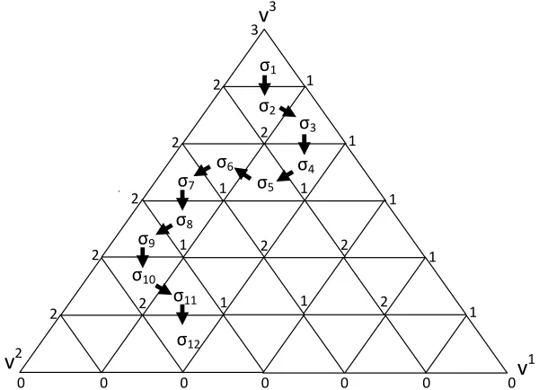
[image:7.612.160.460.84.301.2]v
3Figure 1. TheK-triangulation of 2-simplexS=v1
, v2
, v3
with grid size 6. The small triangles are members of the triangulationK(S,6). The number at a vertex of a simplex in
K(S,6) is the value oflassigned to the vertex and one sees thatl satisfies the assumptions of Lemma 1. The sequence of simplicesσ1, . . . , σ12meets the requirements described in the
proof of Lemma 1.
Definition 2. Letz :int∆n→Rn be an excess demand function, n∈N. A pointp∈int∆n
is called an equilibrium point for z, if z(p) = 0.
The main goal of the paper is to give a new proof of the fact that for each excess demand function there exists an equilibrium point. First, we are going to characterize the behavior of
z near the (relative) boundary of its domain, which is crucial for the theorem to follow. The intuition for the lemma below is as follows: if the pricepi of a goodiis low (in comparison to
some other price - prices are standardized; they sum up to 1) then the demand significantly exceeds the supply of that good; if the price pi is (relatively) high - so all the other prices
Lemma 2. Let z : int∆n → Rn be an excess demand function. Then there exists ε
1 > 0
such that for i∈[n] and p∈int∆n we have
(pi ≤ε1 ⇒zi(p)>0) and (pi ≥1−ε1 ⇒zi(p)<0).
Proof. Suppose that the former implication is not true. Then there exist i ∈ [n] and a
se-quence pj ∈int∆n, j ∈N: lim j→+∞p
j =p,p
i = 0, and lim j→+∞zi(p
j)≤0 - which contradicts the
boundary condition. This implies that there exists ε1 >0 for which the just considered im-plication is true and without loss of generality we can assume that ε1 <1−ε1. To prove the latter implication observe thatpi ≥1−ε1impliespi′ ≤ε1, i6=i′, so the first implication
guar-antees that zi′(p)>0, i′ 6=i. Now, from Walras’ law, we get 0 <Pi′
6
=ipi′zi′(p) = −pizi(p),
and zi(p)<0 is satisfied.
Lemma 3. Let z and ε1 be as in Lemma 2. Let S1 :={p∈int∆n: pn∈(0, 1−ε1/2]} and
define the function ze:int∆n→Rn−1 as follows:
∀p∈int∆n ez(p) := ((1−pn)zi(p) +pnzn(p))ni=1−1. (1)
Then
(1) ez is continuous,
(2) ez is bounded from below: inf
p∈int∆nzei(p)>−∞, i∈[n−1],
(3) p1ez1(p) +. . .+pn−1ezn−1(p) = 0 for p∈int∆n,
(4) if pj ∈ S
1, j ∈ N, lim
j→+∞p
j =p ∈ ∂(∆n) and p
i = 0, i ∈ [n−1], then lim j→+∞zei(p
j) =
+∞,
(5) ∃ε2 ∈(0, ε1/2]∀p∈S1∀i∈[n−1] :
(pi ≤ε2 ⇒zei(p)>0) and (pi ≥1−ε2 ⇒ezi(p)<0).
Proof. The continuity ofez is obvious. The boundedness from below ofez stems from the fact
that z is bounded from below and the weightspn, 1−pn, are positive and less than 1 for all
pn∈(0,1). The following equalities show that property (3) is met:
p1ez1(p) +. . .+pn−1ezn−1(p) =
=p1((1−pn)z1(p) +pnzn(p)) +. . .+pn−1((1−pn)zn−1(p) +pnzn(p)) =
= (1−pn)(p1z1(p) +. . .+pn−1zn−1(p)) + (p1+. . .+pn−1)
| {z }
=1−pn
pnzn(p) =
= (1−pn)pz(p) = 0.
Ifpj ∈S
1, j ∈N, converges to a pointp with pi = 0 for some i∈[n−1] then (1−pjn)zi(pj)
diverges to +∞and since the productpjnzn(pj) is bounded from below it holds: lim j→+∞zei(p
+∞. To prove that (5) is true it suffices to observe that for p ∈ S1 we have 1−pn ≥ ε1/2 and to proceed as in the proof of Lemma 2 with ez in place ofz.
The formula used to define the functionezresembles the linear homotopy between functions
((1−ε1/2)z1(·, ε1/2) + (ε1/2)zn(·, ε1/2))ni=1−1,
and
((ε1/2)z1(·,1−ε1/2) + (1−ε1/2)zn(·,1−ε1/2))ni=1−1;
just puttin place ofpn, assume thattchanges fromε1/2 through 1−ε1/2 and the ’homotopy’ is
H(p1, . . . , pn−1, t) := ((1−t)zi(·, t) +tzn(·, t))ni=1−1. But H is not a homotopy since the domain of H(·, t) changes as t changes.
The important thing - which Lemma 3 reveals - is that at each fixed pn∈(0,1) the function
e
z(·, pn) is an excess demand function defined on a simplex of dimension n−2 instead of
n−1.9
Now suppose that ε1 and ε2 satisfy the statement of Lemma 3 and let for i∈[n]:
ei :=
ε2
n−1, . . . ,
ε2
n−1, 1| {z }−ε2
i−th coordinate
, ε2
n−1, . . . ,
ε2
n−1
∈int∆n. (2)
We can assume that the vectors ei, i ∈ [n], are linearly independent - it suffices to take
sufficiently smallε2 >0. The setS2 :=
ei : i∈[n] ⊂int∆n is an (n−1)-simplex with the verticesei, i∈[n]. If p∈S
2∩S1, then pi ∈[ε2/(n−1),1−ε2], i∈[n−1] and if αpi = 0 (i.e.
pi =ε2/(n−1)< ε1/2) then ezi(p)>0; similarly, ifαpi = 1 (i.e. pi = 1−ε2 >1−ε1/2) then
e
zi(p)<0. Moreover, if p∈S2 and pn ≥1−ε1 then zn(p)<0 and if pn≤ε1 then zn(p)>0
(see Lemma 2). We are now in a position to prove the main result of the paper.
Theorem. Let z be as in Lemma 3. For each ε > 0 there exists p∈int∆n : z
i(p)≤ ε, i∈
[n].
Proof. If n = 1 then there is nothing to prove: int∆1 = {1} ⊂ R and - by Walras’ law - z(p) = 0 at p = 1. Suppose that n ≥ 2. Let us fix ε > 0 and define ε′ := εε
1, where
ε1 comes from Lemma 2. Let also S1 be as in the hypothesis of Lemma 3 and let S2 be the (n − 1)-simplex with vertices given by (2). By the continuity of the restriction of ze to the compact set S2 there exists δ > 0 such that if p, p′ ∈ S2 and |p− p′| < δ, then |ze(p)− ez(p′)| < ε′. Choose an integer m ≥ 2 for which all simplices in K(S
2, m) 9The idea for the definition ofzecomes from the proof of Theorem 1 in [4] as it comes as a loose suggestion
have diameter less than min{δ, ε1/4}. Let k1 denote the smallest integer in [m] for which (1− k1
m) ε2
n−1 + (1−ε2)
k1
m ≥ 1− ε1
2 - this ensures that a point p ∈S2 whose last barycentric coordinate in S2 is greater than or equal to k1/m satisfies pn ≥ 1−ε1/2. To justify this statement, observe that 1−ε2− nε−21 ≥1−2ε2 ≥1−ε1 >0 andαpn≥k1/m entail
pn= (1−αpn)
ε2
n−1 + (1−ε2)α
p n=
ε2
n−1 +
1−ε2−
ε2
n−1
αpn≥
≥ ε2 n−1 +
1−ε2−
ε2
n−1
k1
m =
1− k1 m
ε2
n−1 + (1−ε2)
k1
m ≥1−ε1/2.
The minimality ofk1assures that for any nonnegative integerk < k1ifp∈S2andαpn≤k/m,
then pn<1−ε1/2 andp∈S1 - the latter implies that the claim of Lemma 3.(5) applies to
p. Notice that if p ∈S2 and pn ≥1−ε1/2 then zn(p) <0 and if pn < ε1/2 then zn(p) >0
(see Lemma 2). Let us define a function l from the set of verticesV(S2, m) to [n]∪ {0} as follows:10
l(p) =
n, if αp
n= 1,
0, if αp
n= 0,
min{i∈[n−1] : αpi >0}, if 1> αp
n≥k1/m, min{i∈[n−1] : zei(p)≤0}, if k1/m > αpn>0,
(3)
where zeis defined in (1). For i ∈ [n−1], if p ∈ V(S2, m), 1 > αpn ≥ k1/m, and αpi = 0
then it is clear that l(p) 6=i, since if l(p) =i, then we would obtain αpi > 0. Assume that
p ∈ V(S2, m) and 0 < αpn < k1/m. Since p ∈ int∆n, Lemma 3.(3) ensures that zei(p) ≤ 0
for some i ∈ [n−1] - so, l(p) is well-defined. Moreover, αp
n < k1/m implies αpn = k/m for
some nonnegative integer k such that k < k1 and therefore, due to Lemma 3.(5), it holds that ezi(p) > 0 for αip = 0 from which we obtain l(p) 6= i whenever α
p
i = 0. Therefore, the
assumptions of the combinatorial Lemma 1 are satisfied. Hence, there exists a sequence of simplices σ1, . . . , σJ inK(S2, m) such thatσj andσj+1 are adjacent and n∈l(σ1), 0∈l(σJ),
[n−1]⊂l(σj), j ∈[J]. There exists the first simplex in that sequence, call itσj1, such that
for all j > j1 the last barycentric coordinate of all vertices of σj in S2 are less than k1/m. Simplices σj1 ∩σj1+1 are adjacent, i.e. they share an (n−2)-face, and in other words, they
differ by one vertex only. By the choice ofj1 all verticesp∈V(σj1+1) satisfyα
p
n < k1/m, and there is a vertex p∈V(σj1)\V(σj1+1) such that α
p
n ≥k1/m. Now, the adjacency of σj1 and σj1+1, the fact that all simplices in K(S, m) have diameters less thanε/4 and the inequality pn≥1−ε1/2 entail thatpn≥1−ε1forp∈V(σj1+1) which implieszn(p)<0 forp∈V(σj1+1).
Reasoning analogously we get for the last simplex, σJ, that it holds: zn(p)>0, p∈ V(σJ).
By the choice of j1, all simplices σj, j ≥ j1 + 1, are contained in S1 ∩S2. Moreover, their
e1
p3≥1-ε1
p3≥1-ε2
p3≤1-ε1/2
S1
S2
e2 e1
e3
e2
e3
p3≤ε1
[image:11.612.116.513.83.375.2]p3≤ε2/2
Figure 2. This figure explains the idea of the proof of Theorem for n= 3. Values ofl
assigned to the vertices inV(S2, m) are independent ofez if the considered vertex is above
or on the linep3≤1−ε1/2 - here the second and third row of the formula (3) are used to
define vales ofl. If a vertex is below the linep3≤1−ε1/2 - but not at the bottom ofS2
-thenezis used to compute the value ofl. The thick curve presents a hypothetical sequence of simplicesσ1, . . . , σJ. For vertices of simplices above (p3≥1−ε1)-line (below (p3≤ε1)-line)
values ofznare negative (positive). Ifσj is below (p3≤1−ε1/2)-line then each coordinate
ofzeadmits a non-positive value at a vertex of σj. Somewhere between (p3 ≥1−ε1) and
(p3≤ε1)-lines there is a simplexσj such that zn(p)zn(p′)≤0 for a pair of vertices p, p′ of
σj - that simplex is what we are looking for.
diameters are less thanδsop, p′ ∈σ
j, j ≥j1+1, implies|ezi(p)−zei(p′)| ≤ε′, i∈[n−1]. Since
S
j≥j1σj is (arcwise) connected andV(σj1)∩z−
1
n ((−∞,0)) 6=∅andV(σJ)∩zn−1((0,+∞))6=∅
then - by the continuity of ze - there exists a simplex σj2, j2 ≥ j1 + 1 : 0 ∈ zn(σj2). Let p∈σj2 :zn(p) = 0. So|p−p′|< δ, p′ ∈V(σj2). Since for eachithere exists a vertexp
i ofσ j2
such thatezi(pi)≤0 (by the inclusion [n−1]⊂l(σj2)), (1−pn)zi(p) = ezi(p)≤zei(p
i) +ε′ ≤ε′,
i∈[n−1]. Further, zi(p)≤ ε
′
(1−pn) ≤
ε′
ε1 =ε, i∈[n−1], since pn∈[ε1,1−ε1], ifzn(p) = 0,
due to Lemma 2. We have found a point p ∈ int∆n: z
i(p) ≤ ε, i ∈ [n], which ends the
proof.
Proof. Let εq > 0, q ∈ N, be a sequence converging to 0. In view of the proof of Theorem,
for each q ∈ N there exists a point pq ∈ S2 such that zi(pq) ≤ εq, i ∈ [n]. The
Bolzano-Weierstrass Theorem and compactness ofS2imply that there exists a convergent subsequence
pq′
ofpq, such that lim q′→+∞p
q′
=p∈S2. From the continuity of z it follows thatzi(p)≤0,for
i∈[n]. Since p∈S2 ⊂int∆n, pi >0, i∈[n]. Walras’ law ensures that z(p) = 0.
5. An algorithm for the computation of equilibrium
From the proof of Theorem we can derive the following algorithm for computation of a point p ∈ int∆n satisfying z
i(p) ≤ ε, i ∈ [n], where ε > 0 is a given accuracy level.
The algorithm below uses the function l : V(S2, m) → {0,1, . . . , n} defined in (3) and we reasonably assume that n ≥2.
Step 0: Determine ε1, ε2 satisfying claim of Lemma 2 and Lemma 3.(5), respectively. Fix accuracy level: ε > 0. Find δ > 0 such that if p, p′ ∈ S
2, where S2 is defined as in the proof of Theorem, and |p − p′| < δ then |ze(p) − ze(p′)| < εε
1 and let m ≥ 2 be an integer for which all simplices in K(S2, m) have diameter less than min{δ, ε1/4}. Let σ1 be is as in the proof of Lemma 1 for
S = S2, set F aceV ertices := V(σ1)\{en}, v := en (see formula (2))
and go to step 1.
Step 1: Determine the only vertex v ∈ V(S2, m) such that v 6= v and
hF aceV ertices∪ {v}i ∈K(S2, m). Go to step 2.
Step 2: If hF aceV ertices∪ {v}i ⊂ S1, where S1 is defined in Lemma 3, and
zn(v) > 0 STOP: v satisfies zi(v) ≤ ε, i ∈ [n]. Otherwise, assign
the only element of l−1(l(v))∩F aceV ertices as the value of v. Set
F aceV ertices:= (F aceV ertices\{v})∪ {v} and go to step 1.
Step 0 initializes the necessary parameters for correct course of the algorithm and in fact it is the most difficult part of the algorithm, unless we know some properties of the considered excess demand function (e.g. differentiability, its lower bound or if it is a Lipschitz function on compact subsets ofint∆n). It is easy to determinemif we knowδandε
1- it suffices to take
m≥ min(n{−δ, ε1)√2
1/4}, which is a consequence of the definition of theK-triangulation and the fact
that the diameter of a simplex equals the maximum distance between its vertices. In Steps 1 and 2 sethF aceV erticesiis a face of an element of K(S2, m) such thatl(F aceV ertices) = [n−1]. In Step 2 we check if currently considered simplex hF aceV ertices∪ {v}i, where v
implies that the value of l depends on function ze(see Lemma 3 and formula (3)). If it is the case, and in addition zn(v)>0, then v is what we seek for. If not, we have to find the
next adjacent simplex - to this goal we have to decide which vertex should be removed from
F aceV ertices. To achieve this, we find the vertex v ∈F aceV ertices which bears the same value oflasv and we form the new setF aceV erticessubstitutingv in place ofvand then we repeat the operations. The algorithm succeeds in finding approximate zero in a finite number of iterations due to Lemma 1, the Theorem and its proof. It is worth to emphasize that at a given iteration of the algorithm (Step 1 - Step 2) exactly one new value of l is computed and to proceed on with computations it is sufficient to know only the last simplex - there is no need to remember the earlier stages in the course of the algorithm. Moreover, the values of l need to be computed only at the vertices of the constructed sequence of simplices.
6. Final comments
6.1. The boundary condition. The standard form of the boundary condition imposed on/satisfied by an excess demand functions is:11
pj ∈int∆n, j ∈N, lim j→+∞p
j =p∈∂(∆n), p
i = 0, implies lim
j→+∞max{zi(p
j) : i∈[n]}= +∞.
The difference is that we assume that if the (relative) price of a good i tends to 0, then the excess demand for the goodigoes to +∞. The standard condition claims that if the (relative) price of a good itends to 0, then the excess demand for some good - not necessarilyi - goes to +∞. Our condition is satisfied if there is a consumer with Cobb-Douglas preferences and owns a positive quantity of each good. But even if z is an excess demand function that satisfies the standard boundary condition, we can approximate z (as close as we wish on compact subsets of int∆n) with an excess demand function satisfying the version of the
boundary condition used in the paper - see the below construction of the function zh and
just put there z in place ofg.
6.2. Fixed points of continuous functions defined on the standard simplex. Here we show how to relate a continuous function f : ∆n →∆n and an excess demand function,
for which we can apply our algorithm and we can find approximate fixed points of f. We use a construction by H.Uzawa [9]. Let a continuous function g : ∆n→Rn be defined as
∀x∈∆n : g(x) := f(x)− xf(x) xx x.
Sincexg(x) = xf(x)−xf(x) = 0, then the functiong meets Walras’ law. Let us fix a number
h >0 and define a function zh :int∆n→Rn as
zh(x) = (z1h(x), . . . , znh(x)) := (g1(x) +h((nx1)−1 −1), . . . , gn(x) +h((nxn)−1−1)).
One can easily check that zh is an excess demand function. Now, by the Corollary, we see
that for eachh >0 there exists a point xh ∈int∆n: zh(xh) = 0, written equivalently as
gi(xh) = −h
1
nxh i
−1
, i∈[n].
Leth→0+ andxh →x∈∆n(taking a subsequence if necessary). Ifx
i >0, then gi(x) = 0.
If xi = 0 then nx1h
i → +∞ and
1
nxh
i −1 → +∞, so −h
1
nxh i −1
< 0, but boundedness of
g implies that −h 1
nxh i
−1, h > 0, is bounded. We obtain g(x) ≤ 0, which ensures that
f(x) = x(see [9]). Hence to find an approximate fixed point off we can apply the algorithm for zh, h sufficiently small.
The equivalence of the existence of equilibria for excess demand functions defined on the standard closed simplices12 and Brouwer’s theorem was shown in [9]. The proofs of the equivalence for the excess demand functions considered in the current paper can be found in [5] or [8].
6.3. Open questions. Combinatorial Lemma 1 seems to be interesting for its own sake in spite of the fact that it is proved for a particular triangulation. We have seen that it implies the existence of equilibrium for an excess demand function. A slight modification of the proof of Theorem 7 in [5] allows to claim that the existence of equilibrium for an excess demand function is equivalent to the Brouwer fixed point theorem (see also [8]). The famous Sperner lemma which is a combinatorial tool used to prove Brouwer’s fixed point theorem (and which is equivalent to it [10, p. 21]) has many implications (e.g. see [3, pp. 101-103]). What are other implications of Lemma 1? Does Lemma 1 generalize to any triangulation of the standard simplex? Is it equivalent to Sperner’s lemma? What about the behavior of the algorithm presented in the paper in comparison to the behavior of other computational methods for finding equilibria (e.g. methods presented in [10])? How to modify the algorithm to allow for the computation of (approximate) equilibria of excess demand mappings rather than functions?
References
[1] Aliprantis, Ch, Brown, D, Burkinshaw, O: Existence and Optimality of Competitive Equilibria, Springer, Berlin (1990)
[2] Debreu, G: Existence of Competitive Equilibrium. In: Arrow, KJ, Intriligator MD (eds.) Handbook of Mathematical Economics, vol. 2, pp. 697–743, North-Holland Publishing Company, Amsterdam (1982) [3] Dugundji, J, Granas, A, Fixed Point Theory, Springer, New York (2003)
[4] Ma´ckowiak, P: The existence of equilibrium without fixed-point arguments. J. Math. Econ.46(6),
1194-1199 (2010)
[5] Ma´ckowiak, P: Some equivalents of Brouwer’s fixed point theorem and the existence of economic equilib-rium. In: Mat loka, M (ed.) Quantitative Methods In Economics. Scientific Books, vol. 222, pp. 164–171, Pozna´n University of Economics Press, Pozna´n (2012)
[6] Mas-Colell, A: On The Equilibrium Price Set of an Exchange Economy. J. Math. Econ. 4, 117-126
(1977)
[7] Scarf, H: The Computation of Equilibrium Prices: an Exposition. In: Arrow, KJ, Intriligator MD (eds.) Handbook of Mathematical Economics, vol. 2, pp. 1006–1061, North-Holland Publishing Company, Amsterdam (1982)
[8] Toda, M: Approximation of Excess Demand on the Boundary and Equilibrium Price Set. Adv. Math. Econ.9, 99–107 (2006)
[9] Uzawa, H: Walras’ Existence Theorem and Brouwer’s Fixed-Point Theorem. The Economic Studies Quarterly13(1), 59–62 (1962)
[10] Yang, Z: Computing Equilibria and Fixed Points, Kluwer, Boston (1999)
Department of Mathematical Economics, Pozna´n University of Economics, Al. Niepodleg lo´sci 10, 61-875 Pozna´n, Poland